
Burst Diagnosis Multi-Stage Model for Water Distribution Networks Based on Deep Learning Algorithms


School of Environmental Science and Engineering, Tianjin University, Tianjin 300350, China
*
Author to whom correspondence should be addressed.
Water 2024, 16(9), 1258; https://doi.org/10.3390/w16091258
Submission received: 18 March 2024
/
Revised: 22 April 2024
/
Accepted: 25 April 2024
/
Published: 28 April 2024
(This article belongs to the Special Issue Green and Low Carbon Development of Water Treatment Technology, 2nd Edition)
Abstract
:Pipe bursts in water distribution networks (WDNs) pose significant threats to the safety of distribution networks, driving attention to deep learning-based burst detection and localization. However, the applicability of different pressure features still needs to be compared and verified. A large number of nodes challenges deep learning with the excessive number of classification categories and low recognition accuracy. To address these problems, this paper extracts different burst pressure features, including pressure value, pressure difference, and pressure fluctuation ratio, and inputs one of these features into a Burst Diagnosis Multi-Stage Model (BDMM) based on three CS-LSTMs (a combination of the Cuckoo Search algorithm and a long short-term memory network). The first model addresses a binary classification problem, outputting labels indicating whether a pipe burst has occurred. The second one solves a multi-classification problem, outputting the label of the burst partition, and the third model also solves a multi-classification problem, outputting the ID of the bursting junction. The model is tested on a real network and outperforms ELM. For basic burst identification tasks using CS-LSTM, differences among the three features are minimal, while pressure difference and pressure fluctuation ratio exhibit superior performance to pressure value when resolving more complex problems like burst junction localization.
1. Introduction
Pipe bursts have become a major challenge for water distribution networks (WDNs) because they cause not only a large amount of water loss but also serious service interruptions [1]. Research on the effective diagnosis of pipe bursts is necessary for system operation safety and burst damage control [2].
Currently, there are four primary categories of methods for burst detection in water supply networks: hardware-based techniques, transient-based methods, statistical methods, and hydraulic model-based methods [3]. The hardware-based methods utilize field equipment (e.g., vibroacoustic techniques, listening sticks/correlators, gas injection techniques, thermography, ground-penetrating radar, etc.) to conduct field inspections of WDNs to detect and localize bursts, which is time-consuming and labor-intensive [4]. Transient-based detection methods, on the other hand, primarily focus on analyzing the behavior of transient waves generated by devices. However, acquiring a high-resolution signal often necessitates the procurement of costly pressure-monitoring equipment [5]. The application of the two methods in large WDNs is limited because of the high cost.
With the widespread use of SCADA systems, hydraulic model-based methods and statistical methods have drawn significant attention from researchers. The primary objective of the hydraulic model-based approach is to simulate the operation of WDNs; when discrepancies are observed between the measured data obtained from sensors and the corresponding simulated values, it can be inferred that a burst has occurred [6]. This method can be further subclassified into three categories: sensitivity analysis, optimization calibration, and error-domain model falsification [7]. The accuracy of this method heavily relies on the calibration of the model. Burst diagnosing with this method typically necessitates the use of a real-time hydraulic model and proper model calibration, and it is primarily suitable for small-scale WDNs, which restricts its practical application [8,9].
Statistical methods focus on detecting anomalies by applying data analysis or statistical learning techniques to the collected data [10]. These approaches are particularly suitable for WDNs equipped with a large number of sensors and are not sensitive to the complexity and scale of the WDNs [11]. The recent boom of machine learning and deep learning algorithms has accelerated the application of statistical methods in burst diagnosis. These algorithms, particularly those based on deep learning algorithms, have the unique ability to learn highly complex functions directly from raw data, enabling them to automatically identify the appropriate feature space. For example, Zhou et al. [12] proposed a burst localization framework based on FL-DenseNet, and after optimizing the placement of pressure sensors, the model can effectively identify the location of a pipe burst from potential areas (e.g., District Metering Areas). Cheng et al. [13] built a burst localization framework, first dividing the WDN into monitoring areas based on hydraulic characteristics caused by burst events, then identifying and localizing bursts with a fully linear DenseNet model enhanced by an attention mechanism and Bayesian hyperparameter optimization. A subsequent study replaced FL-DenseNet with FL-ResNet, obtaining comparable average accuracy but with less training time [14]. While deep learning-based methods demonstrate superior accuracy, they rely on mathematical–statistical models which lack explanations and require a large number of burst data. The burst data with flow or pressure features can originate from real monitoring records or bursts simulated by hydraulic modeling software [15]. The use of flow data is generally combined with the District Metering Area (DMA). For example, Lauren et al. [16] used a dataset of more than 2000 DMAs and applied a recurrent neural network to predict the average flow rate, which was then combined with the predicted residuals obtained via real-time Kalman filtering as a method of burst warning. A pipe burst event will result in different magnitudes of pressure decreases across multiple sensors. Therefore, methods for extracting spatio-temporal pressure features can improve the accuracy of burst detection. Shekofteh et al. [17] combined ANN and graph theory with pressure sensor measurements for leak detection and localization. Demand and pressure data can be transformed into images and be learned by conditional, convolutional generative adversarial networks to identify leakage [18].
Hydraulic models and statistical methods, with their upsides and limitations, complement each other, and their combination overcomes nodal demand uncertainty, measurement noise, and the subjectivity of manually defining thresholds for burst detection [19]. Min et al. [20] introduced a two-phase model for leakage detection and localization, where, in the first phase, leakage events are detected through processes involving data categorization, data feature extraction, and data validation. Then, in the second phase, the L-Town hydraulic model is calibrated and the leakage location is determined using a trial-and-error optimization procedure. Soldevila et al. [21] proposed to analyze the inlet flow to detect a leak inside a DMA and then use synthetic data from the hydraulic model to train the classifier for burst localization. A mixed model-based and data-driven method involving seasonal and trend decomposition using loess and the K-means clustering method identified and located 13 of 23 authentic leakage events that existed in L-Town in 2019 [22].
Although existing studies have explored the potential of deep learning methods for pipe burst identification and localization, a notable gap persists in the literature regarding feature extraction employed by intelligent algorithms. Identification and localization of pipe bursts is essentially a process of feature extraction. There is a lack of discussion on the selection of different features and their performance in the task of burst identification and localization. In addition, the number of nodes in real WDNs is large, and the direct use of deep learning methods for the identification and localization of bursts raises issues such as excessive number of classifications and lower accuracy in recognition.
To address the above problems, a multi-task analysis framework for pipe burst diagnosis in a WDN is proposed in this paper, and a Burst Diagnosis Multi-Stage Model (BDMM) is developed based on a combination of LSTM and the Cuckoo Search algorithm (CS-LSTM). After partitioning the WDN and strategically placing pressure sensors, three different pressure features (pressure value, pressure difference, and pressure fluctuation ratio) of monitoring points are extracted. Then, the meta-heuristics Cuckoo Search algorithm is used to optimize hyperparameters related to LSTM. One of the three features is fed to the first optimized LSTM model to output the classification label of whether a pipe burst occurred, and then one of the three features is input into the second LSTM classification model, which outputs the label of the burst partition to determine the partition where the burst occurred, and finally one of the three features is input into the third LSTM classification model, which outputs the ID of the burst junction to pinpoint the node location of the burst. The model is trained and tested using data from a WDN in eastern China and compared with the Extreme Learning Machine method, a traditional machine learning algorithm.
2. Methods
2.1. Overview
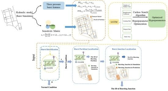
Figure 1 illustrates the framework of this paper, which consists of two steps. (1) Burst pressure feature extraction: the placement of the monitoring system including network partition and pressure sensor arrangement is carried out based on the hydraulic model of WDN; three burst pressure features, namely pressure value, pressure difference, and pressure fluctuation ratio, are calculated, taking into account the variation in hydraulic state and the noise of the pressure sensors. (2) Construction of Burst Diagnosis Multi-Stage Model (BDMM): the BDMM is constructed to identify whether a burst event occurs, determine the burst partition, and finally locate the burst junction based on burst pressure feature data.
2.2. Burst Pressure Feature Extraction
2.2.1. Network Partition and Sensor Layout for Monitoring System
This article adopts K-means clustering as a network partition method. When a pipe burst occurs at a certain node in the water distribution network, it affects the pressure values of other nodes in the network. Therefore, a sensitivity matrix can be defined to characterize the degree of closeness between nodes when a pipe burst occurs in the network and can be used as the input of the K-means algorithm. The output of the K-means algorithm represents the categories of the partition. The calculation of the sensitivity matrix is presented in Equation (1):
where is the sensitivity matrix of the WDN at time t, stands for the pressure of node j when node i experiences a pipe burst in the WDN, denotes the pressure of node j under normal operating conditions at time t in the WDN, means the pressure of node i when node i experiences a burst in the WDN, signifies the pressure of node i under normal operating conditions at time t in the WDN, and s is the number of nodes of the WDN.
Previous studies have primarily utilized data from high-demand days and peak hours for calculating the sensitivity matrix of WDNs. Employing data from various operating conditions provides a more comprehensive representation of the hydraulic status. Therefore, in this study, pipe bursts are simulated for each time step and each node in the WDN. Simultaneously, the pressure values for each node under bursting and the pressure values for the same node under normal working conditions are recorded. The sensitivity matrix of the WDN under various operating conditions is calculated at multiple moments, and after merging, it forms a sensitivity matrix, which is as follows:
The water distribution network is divided into k partitions based on the results of K-means clustering and the topology connection and layout of the pipelines. Each category has a cluster center, which is regarded as the most sensitive to pressure fluctuations during bursts. Therefore, monitoring sensors are installed at the point where the cluster center is located.
Due to the hydraulic status influence of pipe burst, the sensitivity matrices of nodes generated with pipe burst simulation demonstrate significant similarity and strong spatial coherence. However, there may be instances of non-connected nodes in the clustering results with the K-means method. The following strategy is employed to optimize partition boundaries. First, based on the clustering results, the largest connected node set in each cluster is selected as the basis of each partition, while the remaining non-connected nodes are regarded as scattered nodes. Then, each scattered node is assigned to the nearest cluster that the node is topologically connected to. Finally, the boundaries of each network partition are formed based on the results from the above two steps, taking into account the similarity of node sensitivity matrices and also the structure of the water distribution network.
2.2.2. Burst Pressure Features
Burst Simulation
- (1)
- Burst Simulation
Pipe burst simulation is carried out based on the pressure-driven analysis (PDA) model in EPANET 2.2. By assigning the discharge coefficient of emitter c of the node, the pipe burst under different operating conditions is simulated. The discharge coefficient and burst flow are calculated as follows:
where c is the discharge coefficient, AD is the cross-sectional area, n is the loss area ratio (represents the damage degree of pipes), QL is the burst flow, and H is the pressure of the pipe.
- (2)
- Pipe burst conditions
The impact of pipe bursts on the water distribution network varies under different conditions, considering factors such as the severity of the burst, the location of the burst node, and the time of the burst event. To explore these effects, different scenarios are simulated by traversing all nodes and time steps and adjusting the loss area ratios representing varying degrees of pipe burst severity.
- (3)
- Data noise synthesis based on historic monitoring data
Random fluctuation features of the pressure sensors should also be added to the pressure data simulated by EPANET to synthesize the monitoring data of WDN. The pressure values of monitoring points at time t of each day are obtained from data under normal operations in a certain period to create the pressure set . The standard deviation of each monitoring point at time t is also calculated. The mean value of 0 and the standard deviation of are used to generate the normal distribution random matrix which subsequently acts as the noise fluctuation added to the data under burst simulation.
Calculation of Three Different Burst Pressure Features
- (1)
- Pressure Value (PV)
Burst simulation is conducted at each time step and each node with different loss area ratios in turn. is defined as the pressure of monitoring point j when a burst occurs at node i at time t plus the normal distribution random matrix , which is used as the noise fluctuation. can be calculated with Equation (5).
Similarly, is added to the pressure of monitoring point j at time t under normal simulation to obtain the normal pressure value under the influence of noise. The mathematical expression is as follows:
- (2)
- Pressure Difference (PD)
When a burst occurs, the nearby monitoring points will sense a pressure drop. The pressure difference is the pressure of monitoring point j at time t when node i bursts plus the normal distribution random fluctuation minus the average pressure value of the historical data of monitoring point j at time , and the calculation formula is presented in Equation (7).
The calculation of ‘’ needs data with a sufficiently long time span. An example illustrating how ‘’ is calculated as follows: if the duration of simulation is m days and the time step is 1 h, gather the pressures of monitoring point j at the same hour t of these days, and the average of these m numbers is defined as.
- (3)
- Pressure Fluctuation Ratio (PFR)
To reflect the impact of the burst event on the pressure sensors, the pressure fluctuation ratio (PFR) is defined as the proportion of pressure fluctuations, using Equation (8).
where is the pressure fluctuation ratio at monitoring point j when a burst occurs at node i at moment t, and is the average pressure value of historical data at monitoring point j at moment t.
The pressure value (PV) can be obtained directly through the processing of monitoring data, making data acquisition and calculation relatively easy. The pressure difference (PD) and pressure fluctuation ratio (PFR) can highlight the pressure drop of the monitoring point caused by pipe bursts to some extent but require an estimation of the expected pressure value at the monitoring point, which incurs higher calculation costs and introduces uncertainty to pipe burst identification. The impact of the three features on the performance of burst analysis will be compared in the later section.
2.3. Burst Diagnosis Multi-Stage Model
2.3.1. The Architecture of Burst Diagnosis Multi-Stage Model (BDMM)
The Burst Diagnosis Multi-Stage Model (BDMM) consists of three burst diagnosis modules, including the burst identification module, burst partition localization module, and burst junction localization module, as illustrated in Figure 2. The burst identification module is trained with each dataset containing pressure features of normal and burst scenarios. The output of this model is a binary classification, which indicates whether a pipe burst accident has occurred in the WDN. The burst partition localization module is trained with a dataset containing the pressure features of burst scenarios. The output is the label of the partition where the bursting junction is located. The burst junction localization module undergoes training with a dataset only containing the pressure features of burst scenarios. Simultaneously, it receives the label of the partition where the bursting point is located, which is from the burst partition localization module. The output is the ID of the top 5 junctions most likely to experience a burst within the burst partition.
2.3.2. CS-LSTM
In this study, each module of the BDMM uses the Cuckoo Search Algorithm–Long Short-Term Memory (CS-LSTM) neural network as the computing core to analyze the features of the burst. LSTM is optimized and improved on the basis of recurrent neural network (RNN) by introducing three kinds of gates. Before training, the Cuckoo Search algorithm (CS) is applied to optimize the hyperparameters of LSTM, which features global search capabilities and fast convergence, thereby enhancing the performance of LSTM [23,24]. The parameters of the Cuckoo Search algorithm are configured as follows: a discovery probability of 0.2, a population size of 30, and a maximum of 20 iterations. The nest positions were initialized randomly, and the fitness value was determined based on the root mean square error (RMSE). The hyperparameters of the LSTM model, including the number of hidden units, learning rate, regularization coefficient, dropout rate, and batch size, were optimized using the Cuckoo Search algorithm.
2.3.3. Model Performance Indexes
In order to assess the effectiveness of the BDMM, a comprehensive set of evaluation indexes is necessary to characterize its performance. Previous research on performance evaluation has often relied on simple indicators such as accuracy and false positive rate, which may not capture a wide range of information and provide a comprehensive assessment of performance. Therefore, this paper employs five indicators to evaluate burst detection performance: Precision, Recall, False Positive Rate (FPR), and Undetectable Rate (UR). Additionally, for the burst partition localization model, two novel indicators, the precision and recall of burst partition localization, are proposed to account for the distinct performance of the model in each partition. Furthermore, Detection Probability is defined to evaluate the burst junction localization module.
Performance Indexes of Burst Identification Module
The quality of a burst model is not determined by a single index, and it needs to perform well in all dimensions to be applicable in practice. For example, if a model has a high false positive rate, it can lead to a loss of credibility, and the water management company deploying inspections every time it receives an alert would also result in a waste of manpower. So the performance of burst identification is assessed by Precision, Recall, False Positive Rate, and Undetectable Rate, which are calculated by the following equations:
where TP, TN, FP, and FN are the number of true positives, the number of true negatives, the number of false positives, and the number of false negatives respectively. P represents the number of positives and N means the number of negatives.
Performance Indexes of Burst Partition Localization Module
The first index, the precision of burst partition localization (ωn), is used to measure the overall correctness of the model’s predictions for partition n, as shown in Equation (13):
where ωn—the precision of burst partition localization for partition n; —the number of times that both the output of the model and the partition having a real burst are partition n, that is, the correct number of times that the model judges that the burst occurred in partition n; Nn—the number of burst occurrences in partition n predicted by the model.
The second index, the recall of burst partition localization (), is to evaluate the performance of burst partition localization, which is a multi-classification problem:
where —the recall of the burst partition localization for partition n; —the number of times that both the output of the model and the partition having a real burst are partition n, that is, the correct number of times that the model judges that the burst occurred in partition n; Wn—the number of samples with an actual burst in partition n.
Performance Index of Burst Junction Localization Module
Detection Probability () is an index for each partition, which is defined as the probability that the top 5 junctions include the true burst junction in partition n. That is to say, 5 nodes with the highest probability are inspected at one time to identify the bursting node in an experiment, and if these 5 nodes include the bursting node, it is a successful burst localization; otherwise, it is considered as failed. Then is defined and calculated as the number of successful burst localizations divided by the total number of burst experiments in the partition n. The practical meaning of this index is the probability that the 5 nodes the repair crews inspect in one round include the burst junction.
where x—the number of simulated burst events where the burst junction is included in the top 5 junctions in the partition n; X—the total number of simulated burst events.
3. Results and Discussion
3.1. Basic Information of the Study Area
In this study, a District Metering Area (DMA) of an industrial park in eastern China with an 8.2 km2 service area and 16,000 m3 average daily water supply is selected as the research area. The inlets of this DMA are at the starting point of three main vertical trunk pipes. The total length of pipelines above 100 mm is about 24.7 km. The pipe diameters range from 100 mm to 500 mm, with the most commonly used diameter being 300 mm. The elevation is derived from geographic information system data, and the range of node pressure is 20 to 29 m. A relatively complete water consumption measurement and pipe network monitoring system is built in the study area, which uploads user water consumption once an hour. Sixty-one days (1464 h) of water consumption and monitoring data have been collected and the EPANET hydraulic model has been established, which includes 464 nodes, 481 pipes, and 90 major consumer meters, as shown in Figure 3a. The demand of nodes in Figure 3a is at the maximum hourly water demand on the peak day over 61 days.
3.2. Calculation of Burst Pressure Features
According to the method in Section 2.2.1, the WDN is divided into 12 partitions based on the clustering result and topological structure of the network, and each cluster center is designated as the monitoring point to form a monitoring system with 12 monitoring partitions and 12 monitoring points, as shown in Figure 3b.
Figure 4 shows how to construct the matrices of [PV], [PD], and [PFR]. According to the burst pressure feature generation method described in the Section Calculation of Three Different Burst Pressure Features, 464 nodes were traversed in 1464 h for burst simulation, and the loss area ratio n of the burst was a set of four values (0.3, 0.5, 0.7, 1), respectively, so the total number of burst scenarios was 1464 × 464 × 4 = 2,717,184. Random fluctuation is also added according to the distribution of the monitoring data at the corresponding time of the 12 monitoring points to obtain the burst pressure value matrix (), the burst pressure difference matrix (), and the burst pressure fluctuation ratio matrix (). In order to achieve the same magnitude, the normal pressure value matrix () is obtained by vertically repeating the pressure matrix 1000 times and adding random fluctuations. The normal pressure difference matrix () and the normal pressure fluctuation ratio matrix () are also obtained using methods mentioned in the Section Calculation of Three Different Burst Pressure Features.
The six matrices above will be used to generate the dataset for the BDMM.
3.3. The Performance of BDMM
After optimizing LSTM by CS, the LSTM hyperparameters are set as follows: the input layer is set with one sequence input layer; the hidden layer includes one LSTM layer with 452 units; and the output layer is a fully connected layer. The loss function is mean square absolute error (MAE), and adaptive moment estimation (Adam) is applied for optimization. The other hyperparameters are set as follows: the maximum number of iterations is set to 10, the learning rate is set to 0.07, the dropout rate is set to 0.5, and the batch size is set to 546. To compare the performance of CS-LSTM with other machine learning algorithms, a classical machine learning algorithm called Extreme Learning Machine (ELM) is trained by the same training data and evaluated with the same test data.
3.3.1. Performance of Burst Identification Module
The datasets of the burst identification module are , , and , respectively, as shown in Table 1:
Datasets , , and are divided into a training set and a test set in a ratio of 7:3. Dataset is divided into Training Set 1 and Test Set 1 in a ratio of 7:3, dataset into Training Set 2 and Test Set 2, and dataset into Training Set 3 and Test Set 3.
The CS-LSTM model and the ELM model are trained and tested using the same dataset, and the indexes mentioned in the Section Performance Indexes of Burst Identification Module are used to compare the effectiveness of the two models for burst identification. The results are shown in Figure 5:
The following conclusions can be drawn by comparing the burst identification results of CS-LSTM and ELM.
CS-LSTM has a low False Positive Rate and Undetectable Rate, while Precision and Recall are maintained at very high levels, all exceeding 0.97, significantly better than ELM with the input of all three features. This overall evaluation of CS-LSTM indicates that it is more suitable for burst identification.
For binary classification prediction tasks like burst identification, whether pressure feature processing is conducted at the input end has little impact on the performance of CS-LSTM. Therefore, pressure value, with no need for the estimation of the mean value of the monitoring point, should be used in burst identification to save computation costs.
3.3.2. Performance of Burst Partition Localization Module
The sample datasets of the burst partition localization module are , , and , as shown in Table 2. They are divided into training sets and test sets in a ratio of 7:3. is the label of the burst partition.
Like the previous section, this study compares the performances of CS-LSTM and ELM. The precision and recall of the partition localization can be obtained from two methods of CS-LSTM and ELM, respectively. The results are shown in Figure 6.
The following conclusions can be obtained by comparison.
Under different feature inputs, the burst partition localization performance of CS-LSTM is significantly better than that of ELM. The average recall and precision of burst partition localization when using CS-LSTM are both above 90%.
For the CS-LSTM model, the average precision when using burst pressure, pressure difference, and pressure fluctuation ratio as inputs is 0.903, 0.930, and 0.913, respectively. The differences among them are small, indicating that simpler pressure data can be used as inputs to reduce computation costs. For the ELM model, the average precision when using burst pressure, pressure difference, and pressure fluctuation ratio as inputs is 0.676, 0.741, and 0.726, respectively. When using pressure difference and pressure fluctuation ratio as inputs, the performance is significantly improved, indicating that the ELM model requires more prominent burst pressure features as inputs to ensure precision compared to CS-LSTM, which requires more complex input features.
When the model is applied to the real burst analysis, only the results of the model output are available, without information on the actual location of the burst. The precision of the burst partition localization in each partition is based on the model output in that partition, so its operability and verifiability are better than those of the burst partition recall, with a higher degree of confidence.
3.3.3. Performance of Burst Junction Localization Module
An independent burst junction localization model is established for each partition, and there are 12 burst junction localization models in total. Figure 7 shows an example in this case to explain how to locate the bursting junction and calculate DP5,n. In this example, the bursting junction ranks fifth, because the top five nodes at one time are inspected to identify the bursting node in an experiment, so this burst junction localization is a success. After all experiments are finished, DP5,n is defined as the number of successful burst localizations divided by the total number of experiments in the partition n.
The datasets of the burst junction localization model are , , and , respectively, as shown in Table 3, and are divided into training and test sets in a ratio of 7:3. is the ID of the burst junction. DP5 of CS-LSTM and ELM is illustrated in Figure 8.
The following conclusions can be obtained by comparison.
For the task of burst junction localization, CS-LSTM outperforms ELM regardless of which feature is utilized among the three features. When using burst pressure, pressure difference, and pressure fluctuation ratio as inputs, the CS-LSTM model achieves an average DP5 of 0.854, 0.966, and 0.945, respectively. The repair crews have more than a 92% probability of locating the burst junction by simply searching for five junctions from the output.
For the CS-LSTM model, when using burst pressure value, pressure difference, and pressure fluctuation ratios as inputs, the average DP5 values are 0.854, 0.966, and 0.945, respectively. The effects of pressure difference and pressure fluctuation ratio are better than those of pressure value. Similarly, for the ELM model, the effects of pressure difference and pressure fluctuation ratio are also better than those of pressure value. This indicates that feature extraction is beneficial for improving the performance of deep learning and machine learning models when dealing with more complex classification problems.
4. Conclusions
In this paper, a novel framework named Burst Diagnosis Multi-Stage Model (BDMM) based on CS-LSTM is proposed to achieve comprehensive burst diagnosis including identifying the burst event and locating the burst partition and junction in WDNs. Three burst pressure features (pressure value, pressure difference, and pressure fluctuation ratio) are constructed and used as inputs of the BDMM, offering insights into feature applicability and model effectiveness for practical WDN applications. The results show that the proposed method can effectively identify pipe bursts and accurately locate them in this case, reducing the deep learning algorithm’s classification complexity and improving localization accuracy. Pressure value should be used for burst identification and partition localization to reduce computation costs, and pressure difference should be used for burst junction localization for better precision in the BDMM. Although the BDMM was trained and validated using simulated data effectively, further study is recommended to validate the model’s effectiveness using real-world measured pipe burst data and to implement it on more complex WDNs, comparing it with other research methodologies.
Author Contributions
S.P.: Guiding the construction of the framework, revising and reviewing the manuscript. Y.W.: Organizing the framework and writing the original draft. X.F.: Generating simulation data and training the model. Q.W.: Building the hydraulic model. All authors have read and agreed to the published version of the manuscript.
Funding
This research was funded by the National Key R&D Program of China, grant number 2022YFC3203803.
Data Availability Statement
The data used in this manuscript are available by writing to the corresponding authors.
Acknowledgments
Thanks to the National Key R&D Program of China for supporting and funding this project under grant number 2022YFC3203803.
Conflicts of Interest
The authors declare that they have no conflicts of interest.
References
- Jun, S.; Lansey, K.E. Convolutional Neural Network for Burst Detection in Smart Water Distribution Systems. Water Resour. Manag. 2023, 37, 3729–3743. [Google Scholar] [CrossRef]
- Qi, Z.; Zheng, F.; Guo, D.; Maier, H.R.; Zhang, T.; Yu, T.; Shao, Y. Better Understanding of the Capacity of Pressure Sensor Systems to Detect Pipe Burst within Water Distribution Networks. J. Water Resour. Plann. Manag. 2018, 144, 04018035. [Google Scholar] [CrossRef]
- Wan, X.; Kuhanestani Parisa, K.; Farmani, R.; Keedwell, E. Literature Review of Data Analytics for Leak Detection in Water Distribution Networks: A Focus on Pressure and Flow Smart Sensors. J. Water Resour. Plann. Manag. 2022, 148, 03122002. [Google Scholar] [CrossRef]
- Kammoun, M.; Kammoun, A.; Abid, M. Leak Detection Methods in Water Distribution Networks: A Comparative Survey on Artificial Intelligence Applications. J. Pipeline Syst. Eng. Pract. 2022, 13, 04022024. [Google Scholar] [CrossRef]
- Che, T.-C.; Duan, H.-F.; Lee, P.J. Transient wave-based methods for anomaly detection in fluid pipes: A review. Mech. Syst. Signal Process. 2021, 160, 107874. [Google Scholar] [CrossRef]
- Pérez, R.; Puig, V.; Pascual, J.; Quevedo, J.; Landeros, E.; Peralta, A. Methodology for leakage isolation using pressure sensitivity analysis in water distribution networks. Control Eng. Pract. 2011, 19, 1157–1167. [Google Scholar] [CrossRef]
- Nimri, W.; Wang, Y.; Zhang, Z.; Deng, C.; Sellstrom, K. Data-driven approaches and model-based methods for detecting and locating leaks in water distribution systems: A literature review. Neural Comput. Appl. 2023, 35, 11611–11623. [Google Scholar] [CrossRef]
- Lee, S.J.; Lee, G.; Suh, J.C.; Lee, J.M. Online Burst Detection and Location of Water Distribution Systems and Its Practical Applications. J. Water Resour. Plan. Manag. 2016, 142, 04015033. [Google Scholar] [CrossRef]
- Sanz, G.; Pérez, R. Sensitivity Analysis for Sampling Design and Demand Calibration in Water Distribution Networks Using the Singular Value Decomposition. J. Water Resour. Plan. Manag. 2015, 141, 04015020. [Google Scholar] [CrossRef]
- Corzo, C.M.; Alfonso, L.; Corzo, G.; Solomatine, D. Locating Multiple Leaks in Water Distribution Networks Combining Physically Based and Data-Driven Models and High-Performance Computing. J. Water Resour. Plan. Manag. 2023, 149, 04023066. [Google Scholar] [CrossRef]
- Jian, C.; Gao, J.; Xu, Y. Anomaly Detection and Classification in Water Distribution Networks Integrated with Hourly Nodal Water Demand Forecasting Models and Feature Extraction Technique. J. Water Resour. Plan. Manag. 2022, 148, 04022059. [Google Scholar] [CrossRef]
- Zhou, X.; Tang, Z.; Xu, W.; Meng, F.; Chu, X.; Xin, K.; Fu, G. Deep learning identifies accurate burst locations in water distribution networks. Water Res. 2019, 166, 115058. [Google Scholar] [CrossRef] [PubMed]
- Cheng, J.; Peng, S.; Cheng, R.; Wu, X.; Fang, X. Burst Area Identification of Water Supply Network by Improved DenseNet Algorithm with Attention Mechanism. Water Resour. Manag. 2022, 36, 5425–5442. [Google Scholar] [CrossRef]
- Takudzwa Sikumbuzo, M.; Clement, N.N. A Comparison of Fully-Linear Deep Learning Methods for Pipe Burst Localization in Water Distribution Networks. In Proceedings of the 2023 IST-Africa Conference (IST-Africa), Tshwane, South Africa, 31 May–2 June 2023. [Google Scholar] [CrossRef]
- Birek, L.; Petrovic, D.; Boylan, J. Water leakage forecasting: The application of a modified fuzzy evolving algorithm. Appl. Soft Comput. 2014, 14, 305–315. [Google Scholar] [CrossRef]
- Lauren, M.; Jawad, F.; Liz, V. Flow Forecasting for Leakage Burst Prediction in Water Distribution Systems using Long Short-Term Memory Neural Networks and Kalman Filtering. Sustain. Cities Soc. 2023, 99, 104934. [Google Scholar] [CrossRef]
- Shekofteh, M.; Jalili Ghazizadeh, M.; Yazdi, J. A methodology for leak detection in water distribution networks using graph theory and artificial neural network. Urban Water J. 2020, 17, 525–533. [Google Scholar] [CrossRef]
- Rajabi, M.M.; Komeilian, P.; Wan, X.; Farmani, R. Leak detection and localization in water distribution networks using conditional deep convolutional generative adversarial networks. Water Res. 2023, 238, 120012. [Google Scholar] [CrossRef] [PubMed]
- Romero-Ben, L.; Alves, D.; Blesa, J.; Cembrano, G.; Puig, V.; Duviella, E. Leak detection and localization in water distribution networks: Review and perspective. Annu. Rev. Control 2023, 55, 392–419. [Google Scholar] [CrossRef]
- Min, K.W.; Kim, T.; Lee, S.; Choi, Y.H.; Kim, J.H. Detecting and Localizing Leakages in Water Distribution Systems Using a Two-Phase Model. J. Water Resour. Plann. Manag. 2022, 148, 04022051. [Google Scholar] [CrossRef]
- Soldevila, A.; Boracchi, G.; Roveri, M.; Tornil-Sin, S.; Puig, V. Leak detection and localization in water distribution networks by combining expert knowledge and data-driven models. Neural Comput. Appl. 2022, 34, 4759–4779. [Google Scholar] [CrossRef]
- Zhirong, L.; Jiaying, W.; Hexiang, Y.; Shuping, L.; Tao, T.; Xin, K. Fast Detection and Localization of Multiple Leaks in Water Distribution Network Jointly Driven by Simulation and Machine Learning. J. Water Resour. Plann. Manag. 2022, 148, 05022005. [Google Scholar] [CrossRef]
- Srivastava, D.; Singh, Y.; Sahoo, A. Auto Tuning of RNN Hyper-parameters using Cuckoo Search Algorithm. In Proceedings of the 2019 Twelfth International Conference on Contemporary Computing (IC3), Noida, India, 8–10 August 2019; pp. 1–5. [Google Scholar]
- Yang, X.S.; Deb, S. Engineering optimisation by cuckoo search. Int. J. Math. Model. Numer. Optim. 2010, 1, 330–343. [Google Scholar] [CrossRef]
Figure 1.
Flowchart of the proposed method.

Figure 2.
Schematic of BDMM structure.

Figure 3.
(a) The WDN of the study area. (b) The partition and monitoring system of the study area.

Figure 4.
The structure of matrices PV, PD, and PFR.

Figure 5.
Evaluation results of burst identification module.

Figure 6.
Performance comparison of CS-LSTM and ELM for burst partition localization.

Figure 7.
An example of how to locate the bursting junction.

Figure 8.
Comparison of CS-LSTM and ELM on the performance of burst junction localization.


Table 1.
Datasets of the burst identification module.
| Dataset | Math Representation |
|---|---|
Table 2.
Datasets of the burst partition localization module.
| Dataset | Math Representation |
|---|---|
Table 3.
Datasets of the burst junction localization module.
| Dataset | Math Representation |
|---|---|
Disclaimer/Publisher’s Note: The statements, opinions and data contained in all publications are solely those of the individual author(s) and contributor(s) and not of MDPI and/or the editor(s). MDPI and/or the editor(s) disclaim responsibility for any injury to people or property resulting from any ideas, methods, instructions or products referred to in the content. |
© 2024 by the authors. Licensee MDPI, Basel, Switzerland. This article is an open access article distributed under the terms and conditions of the Creative Commons Attribution (CC BY) license (https://creativecommons.org/licenses/by/4.0/).
Share and Cite
MDPI and ACS Style
Peng, S.; Wang, Y.; Fang, X.; Wu, Q. Burst Diagnosis Multi-Stage Model for Water Distribution Networks Based on Deep Learning Algorithms. Water 2024, 16, 1258. https://doi.org/10.3390/w16091258
AMA Style
Peng S, Wang Y, Fang X, Wu Q. Burst Diagnosis Multi-Stage Model for Water Distribution Networks Based on Deep Learning Algorithms. Water. 2024; 16(9):1258. https://doi.org/10.3390/w16091258
Chicago/Turabian StylePeng, Sen, Yuxin Wang, Xu Fang, and Qing Wu. 2024. "Burst Diagnosis Multi-Stage Model for Water Distribution Networks Based on Deep Learning Algorithms" Water 16, no. 9: 1258. https://doi.org/10.3390/w16091258
Note that from the first issue of 2016, this journal uses article numbers instead of page numbers. See further details here.