Flood Water Depth Prediction with Convolutional Temporal Attention Networks

Abstract

Robust and accurate flood hazard maps are essential for early warning systems and flood risk management. Although physically based models are effective in estimating pluvial flooding, the computational burden makes them difficult to use for real-time flood prediction. In contrast, data-driven models can provide faster flood predictions if trained offline. While most studies have focused on predicting maximum water depth, in this study, we predict pixel-wise water depth maps for entire catchments at a lead time of 2 h. To that end, we propose a deep learning approach that uses a sequence encoding network with temporal self-attention. We also adapt the popular hydrological performance metric Nash–Sutcliffe efficiency (NSE) as our loss function. We test the effectiveness and generalizability of our method using a new dataset called SwissFlood, which consists of 100 catchments and 1500 rainfall events extracted from real observations in Switzerland. Our method produces 2 m spatial resolution flood maps with absolute error as low as 27 cm for water depth exceeding 1 m.

1. Introduction

Flooding is considered one of the most catastrophic natural hazards and with climate change, this natural hazard is predicted to become more prevalent and drastic [1]. Extreme rainfall and flood events have risen more than $50\%$ globally this decade [2]. This growing frequency of flood events underscores the importance of having dependable strategies for mitigating floods. Flood modelling is an important tool for such a task.

The utilisation of two-dimensional (2D) physically based hydrodynamic models has been prevalent in predicting urban floods. Despite their effectiveness in predicting urban floods, they are computationally expensive which makes it difficult to use them for real-time flood forecasting [3,4]. Although high-performance computing technology has advanced over the years and new computational methods have been developed there are still significant challenges in using these for operational flood forecasting [3]. Cellular automata models were introduced to improve the computational speed of physically based models and make them compatible with parallel processing.

In the last decade, machine learning has emerged as an effective alternative to physically-based models [5,6,7,8,9,10]. machine learning models are not as computationally expensive and still produce useful and accurate results for real-time flood forecasting [4,11]. Given sufficient example data, machine learning models aim to learn the mapping from the observable input to the desired output without explicitly taking into account the underlying physical processes. In particular, deep learning constitutes a form of representation learning, where one aims to learn data representations that are well suited for the associated predictive modelling. It involves the composition of numerous nonlinear transformations to generate more abstract and eventually more helpful representations [12,13]. Deep learning requires a significant amount of training data to fit the model. However, once trained, the model can quickly perform predictions in a single forward pass. If trained on a large, diverse dataset that is representative of the underlying distribution, deep learning models generalise rather well to unseen data. This reduces the need for case-specific calibration when a flood event occurs, unlike hydrodynamic models that often require manual fine-tuning. Both classical and deep machine learning models have been employed for flood analysis and prediction [4,5,8,10,14,15,16].

The main contributions of our study can be summarised as follows:

• We propose a deep learning approach that predicts water depths at high spatial resolution for a two-hour lead time, given elevation data, water depth at starting time, and rainfall intensity values for the forecast duration.
• We introduce the new, large-scale pluvial flood dataset SwissFlood (which is available for download at https://doi.org/10.5281/zenodo.7797844) and make it publicly available. It contains pluvial floods for 100 catchments in Switzerland generated with a hydrodynamic flood model [17]. The rainfall events were extracted from rainfall observation data of the last forty years collected in Switzerland by MeteoSwiss [18].
• In our study, we aim to analyse the ability of our data-driven model to generalise the prediction of future water depth across catchments and rainfall events. All rainfall events used in this study are unique. We provide a quantitative as well as a qualitative analysis of our approach to evaluate its performance.

We illustrate the comprehensive workflow of our method in Figure 1. Our process starts with the acquisition of DEM data for catchments, as well as a collection of diverse rainfall events. From the data gathered from three meteorological stations between 1981 and 2021, we chose 380 rainfall events for our analysis. Additionally, to ensure the model is unbiased with respect to the rainfall intensity, we added and subtracted small random values from rainfall events. With this approach, we generate 1500 unique rainfall events. Employing both the digital elevation model (DEM) data and the identified rainfall events, we simulate the water depth over a span of five hours with the CADDIES 2D cellular automata flood model [17]. Subsequently, we divide our dataset into three mutually exclusive partitions: training, validation, and test sets. We train a variant of the UTAE [19] model (see Section 4.1 for more details) using the training set and find hyperparameters that maximise predictive skill on the validation set. Subsequently, the model is tested on the hitherto unseen test set, producing water depth predictions with a lead time of two hours.

2. Related Work

It is important to generate precise flood predictions for flood risk warnings and to support decision-making and ultimately mitigate flood risks [20]. Traditionally, flood hazard maps are obtained using numerical methods which are robust and effective, but not fast and accurate [21]. Due to the fact that not all sub-processes of the hydrological cycle can be accurately explained, those models include simplifications that may result in simulation errors [22]. The alternative is to use data-driven models based on machine learning, which have become more common during the last decade [23]. For feature extraction, traditional machine learning algorithms need meticulous engineering and significant domain knowledge. In contrast, deep learning methods automatically discover a latent data representation that supports the prediction task. These multi-layered sets of “attributes” are derived in a data-driven fashion, an approach that has proven highly effective in detecting intricate patterns in high-dimensional data, across a wide range of scientific disciplines [12].

Recently, with the growth of public data sharing over the internet, research has been conducted about utilising images as a basis for flood estimation [24,25]. In several studies, such as [26,27,28], the use of social media images combined with deep neural network models has shown potential in predicting flood levels. Another interesting work is [29] where existing surveillance camera systems are used to predict flood level trends. It has the advantage that camera networks exist in many municipalities, with high operational reliability. Drawbacks include a lack of control over the camera placement and privacy concerns. Additionally, Lütjens et al. [30,31] investigated unsupervised learning techniques to produce flood images after an event, given images before the flood event and a flood extent map. Another line of research [32] has explored the potential of reinforcement learning, training a model to actively regulate pond levels using present and predicted events in (artificial) urban catchments.

The recent work has highlighted the potential of flood modelling with data-driven approaches. In [8,14], a convolutional neural network (CNN) is adopted to predict the maximum water depth and velocity of the catchment area based on rainfall and elevation data. Another work Löwe et al. [5] used U-Net to predict 2D maps of maximum flood depth for the city of Odense, Denmark, complemented by an exhaustive assessment of which spatial input variables should be considered. A modified version of U-Net with self-attention is also proposed in Yokoya et al. [10] to regress maximum water levels for simulated disaster scenarios. Berkhahn et al. [7] design an artificial neural network ensemble for predicting maximum water levels based on precipitation forecasts. Similarly, ref. [1] predict maximum flood levels with a novel physics-guided deep learning method that uses a conditional generative adversarial network (cGAN). They first use the cGAN model to identify wet cells and then estimate their water depths. Deep neural networks are often perceived as black boxes; to address this issue, Chaudhary et al. [33] proposed a probabilistic deep learning approach that predicts maximum water depth along with a well-calibrated uncertainty estimate for every water depth. That value indicates how reliable the water depth predictions are. All these studies predict only the maximum water depth [34], whereas our present work aims to predict pixel-wise water depth maps for the entire catchment area with some lead time. Ivanov et al. [35] present an innovative flood forecasting method that performs complex analysis of information on flooding impacts well before a future storm event, with example results for Hurricane Harvey flooding in Houston, USA. In [36], a PredRNN model is trained to emulate the transient, three-dimensional integrated hydrological model ParFlow. Muñoz et al. [37] fuse multi-spectral imagery using a CNN trained and evaluated on the Hurricane Matthew event to produce flood maps at 30 m spatial resolution. Kao et al. [38] develop a method that uses a stacked autoencoder (SAE) to compress and reconstruct flood inundation depth and a recurrent neural network (RNN) to forecast flood features on 31 historic and 24 designed rainfall events with a 40 m grid resolution. Chang et al. [39] develop datasets of rainfall intensity hyetographs and simulated inundated water depths, and use similarities between rainfall patterns to search and retrieve the associated flood depths, so as to promptly predict the potential pluvial flood. Hu et al. [6] combine the long short-term memory (LSTM) framework with a reduced order model (ROM) to perform predictive and prescriptive analytics for the Okushiri tsunami test case.

Lin et al. [40] have developed a multi-step flood forecast method for their study area of Kulmbach, Germany with a spatial resolution of 4 × 4 m². They employ an artificial neural network (ANN) that ingests seven inflows to the study area and returns corresponding output inundation maps at 3, 6, 9 and 12 h. In comparison to our work, that study focuses on a single catchment area, whereas we train and test our method across 100 different catchments. Their approach was also trained on synthetic floods and tested on three historical events, while our rainfall events are extracted from the real precipitation records of Switzerland. We use an attention-based network that is adept at identifying complex temporal patterns and predicting water depth in the form of 2D maps for the catchment area. Another work closely related to ours is [41], where the authors use a Random Forest (RF) as a surrogate model for urban flood predictions. The model was trained on the most prone as well as all 16,914 road segments in the coastal city of Norfolk, USA, and tested in the same city. Moreover, rainfall features like hourly rainfall, maximum 15 min rainfall in an hour, etc. were used as input to the RF, whereas our deep learning model only receives the rainfall intensity per 10 min interval as input.

3. Datasets

3.1. Catchments

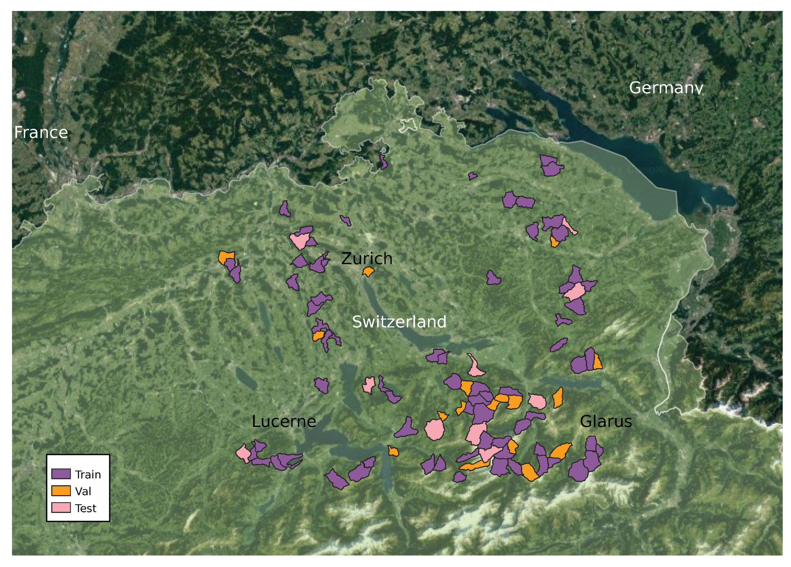
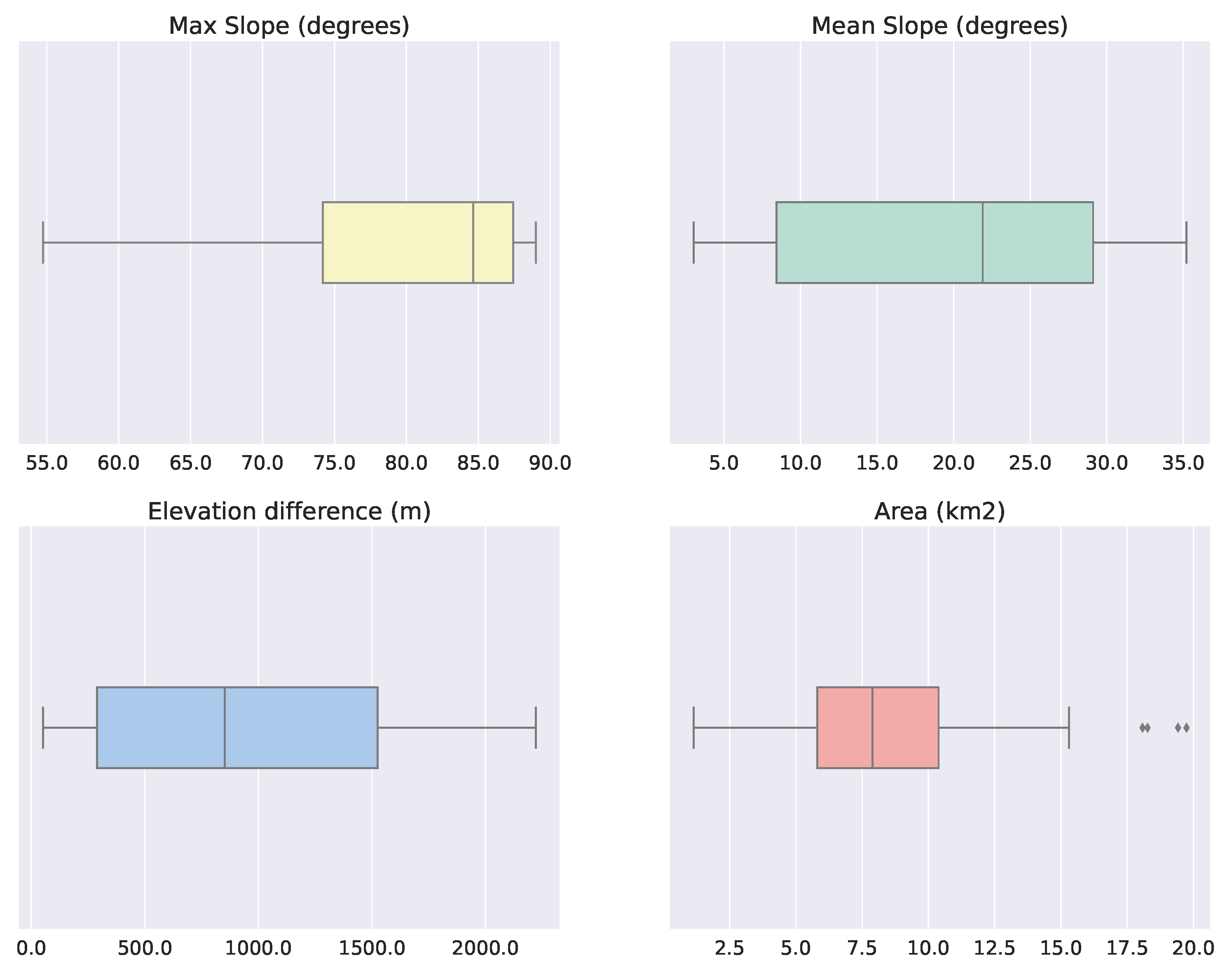
We consider 100 catchments in Switzerland for our case study. These include urban, rural and mixed types of catchments. The elevation data, in the form of gridded DEMs with 2 m grid spacing, were taken from [14], who in turn obtained them by collecting the original data from the Swiss national mapping agency (swisstopo). The different catchment areas in our SwissFlood dataset and their spatial distribution are shown in Figure 2, where violet colour denotes catchments in the training set, yellow denotes the validation set and pink denotes the test set. Additionally, we also show the terrain characteristics of the selected catchments: Figure 3 shows statistics of catchment area (km²), mean and maximum slopes (degrees) and maximum elevation difference (m).

3.2. Rainfall Data

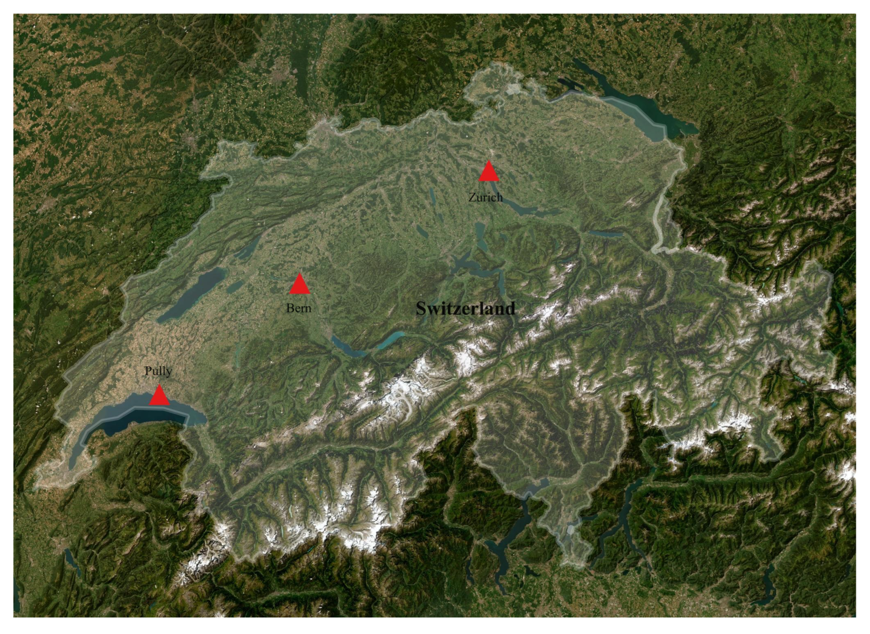
The rainfall events used in our study were collected from the Federal Office of Meteorology and Climatology in Switzerland [18]. We examined the rainfall observations at three meteorological stations, Bern/Zollikofen, Pully, and Zürich/Kloten shown in Figure A1. We analysed the data from 1981 until 2021 at each station and identified suitable rainfall events for generating simulations for the Swissflood catchments. From each station, we selected a diverse range of rainfall events spanning a duration of five hours. We divided these 380 rainfall events into three ranges based on their volume: >40 mm, 30–40 mm, and <30 mm within five hours. Ideally, the machine learning model should be able to predict water depth for large rainfall events as well as for rainfall events that cause mild or no flooding. To adequately cover the range from substantial to no flooding, we have selected seven, five, and three rainfall events, respectively, from the >40 mm, 30–40 mm, and <30 mm ranges. Overall, those events correspond to return periods from below 1 year to ≈50 years. The temporal resolution of the hyetographs is 10 min, and we assume spatially uniform rainfall across catchments. To avoid a bias towards specific intensity values, we add small random perturbations up to ±10% to the observed values. With that approach, we generate 1500 unique rainfall events for all catchments, in order to learn a model that generalises across different events. Exemplary hyetographs are shown in Figure 4. Events tr35_121, tr35_343 were originally observed at the Pully meteorological station, and the remaining events were selected from the Bern/Zollikofen station. The hyetographs in Figure 4 depict several distinct rainfall patterns present in SwissFlood, including single peaks and double peaks. This diversity of precipitation patterns enables our model to generalise to new, unseen events.

3.3. Water Depth

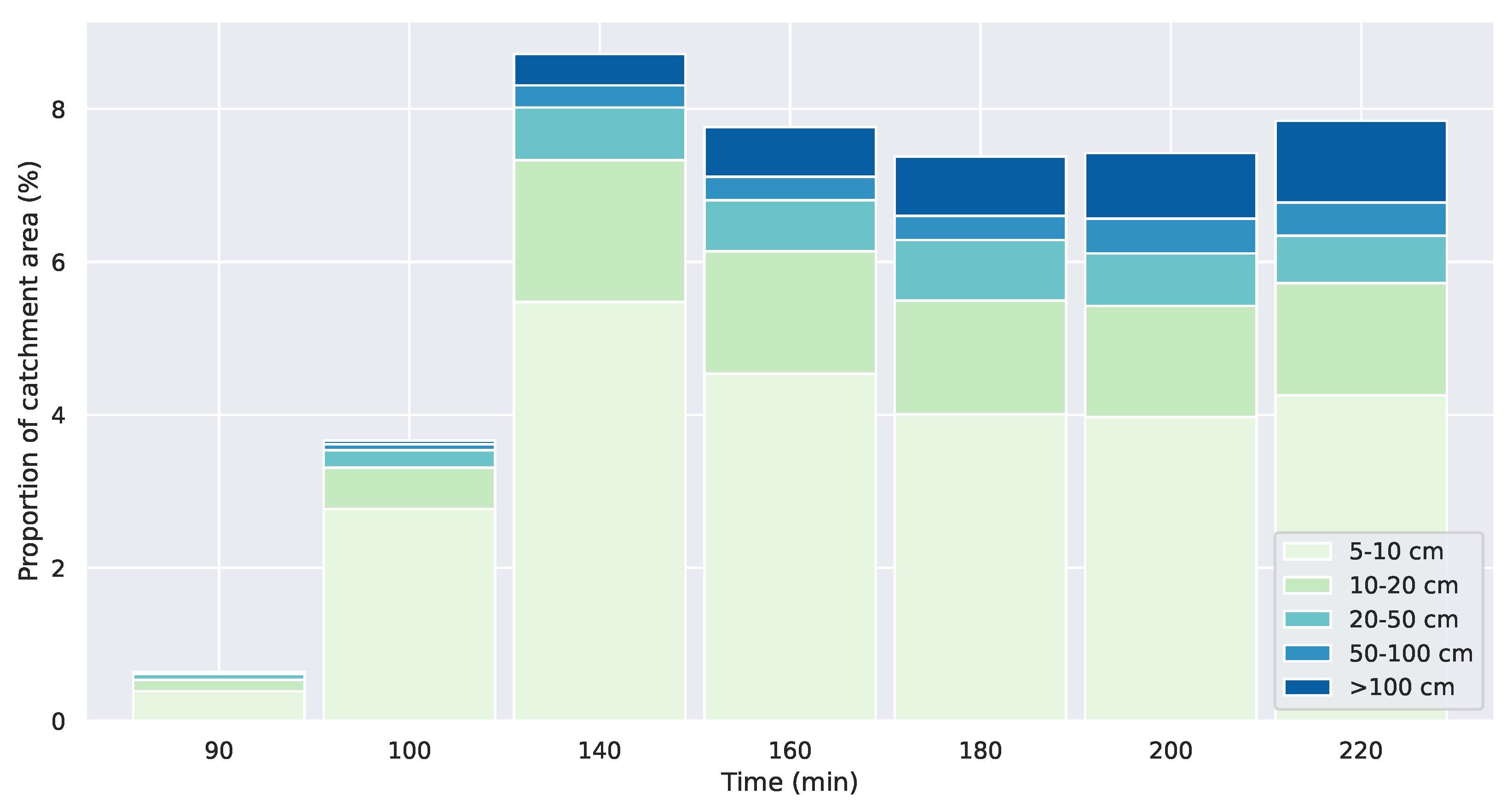
With the Swissflood catchment and rainfall data described above, we drive simulations with the CADDIES 2D cellular automata flood model [17] to generate the reference water depths for machine learning. CADDIES improves upon the methodology used in [42] and employs a weight-based approach to simplify the transition rules that determine the flow movement, thereby reducing the need for complex and computationally demanding numerical solvers. CADDIES is a lot faster than models that solve shallow water equations (SWE), with little loss of accuracy: $R^2$ values between the two solutions at 2 m resolution remain >0.95 [17]. Using the CADDIES model enables us to generate a much larger dataset in an acceptable time. Figure 5 depicts the distribution of water depths for a specific example, namely rainfall event tr35_343 over catchment 809, which has an area of 12.88 km² spanning elevations between 357 m 702 m a.s.l. The event is shown in Figure 4 and has two peaks with intensities up to 60 mm/h. The dominant water depth of 0–5 cm has been omitted to keep the bar chart readable, and that portion can be calculated by completing the bar heights to 100. As expected, there are no locations with depths >50 cm at the beginning of the rainfall event, but that percentage gradually increases with time.

4. Methodology

The present paper focuses on the development of a data-driven method for flood depth prediction with a lead time of two hours, and able to generalise across different terrain characteristics and rainfall events. In other words, the model should be able to predict the water depth for catchments it has not seen during training and validation, and for previously unobserved rainfall events.

We cast the task to predict spatially explicit flood depth maps as a supervised learning problem. The input provided to our neural network are:

• A raster map of terrain elevations for catchment c.
• Water depth at time-step ${\mathbf{wd}}_t$ for catchment c.
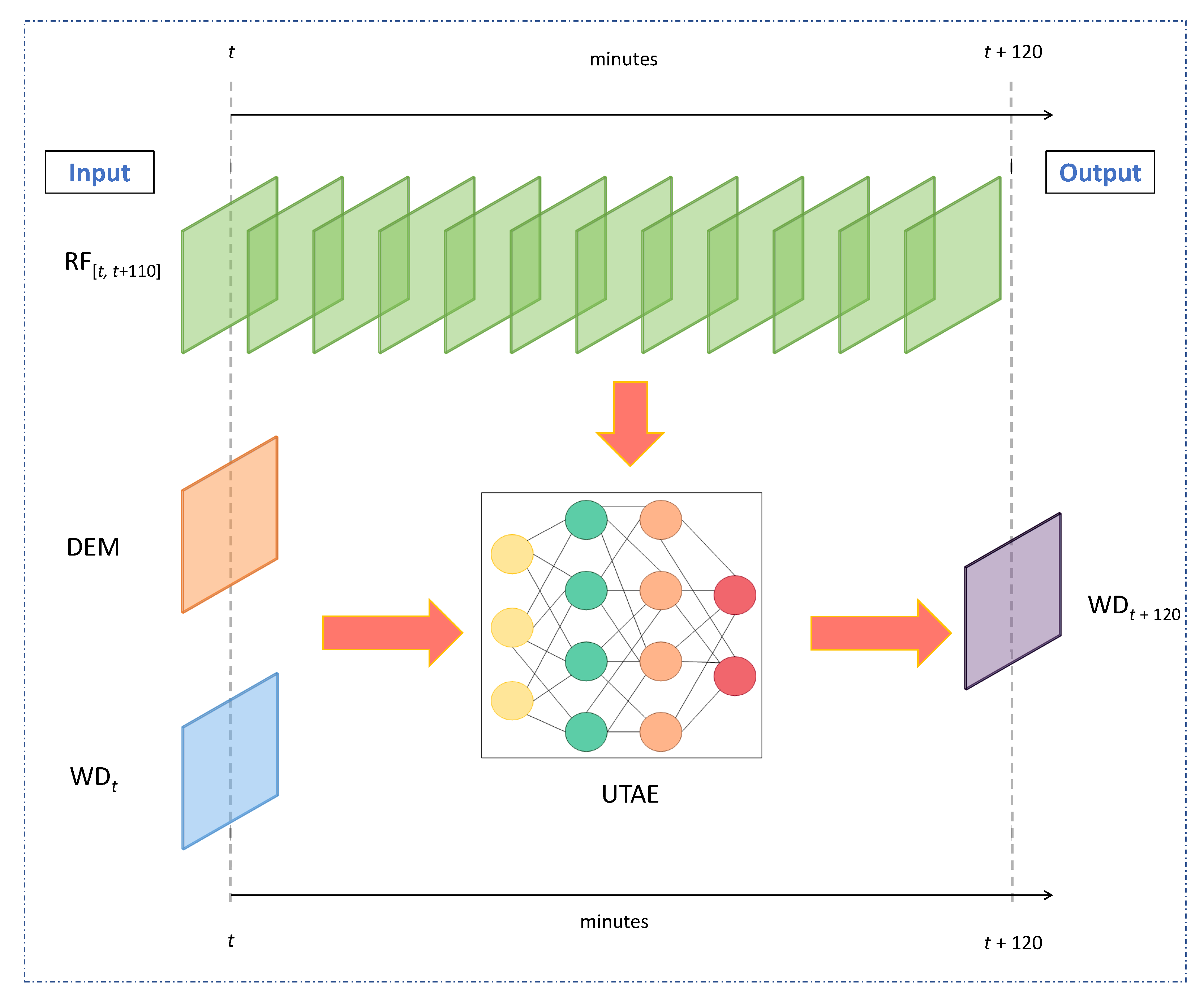
• Rainfall intensity values for the two-hour time window between starting time t and target time $t+120$. The intensity is discretised to steps of 10 min, i.e., the input consists of 12 rainfall values $[{\mathbf{r}}_t,{\mathbf{r}}_{t+10},{\mathbf{r}}_{t+20},\cdots ,{\mathbf{r}}_{t+110}]$.

The output of the trained model is water depth with a spatial resolution of 2 m after two hours, ${\mathbf{wd}}_{t+120}={\mathbf{wd}}_{end}$, as shown in Figure 6. Compared to other studies [5,8,14], we do not extract any hand-crafted features from the data but instead let the model learn the necessary feature extraction during training.

4.1. Deep Learning Model

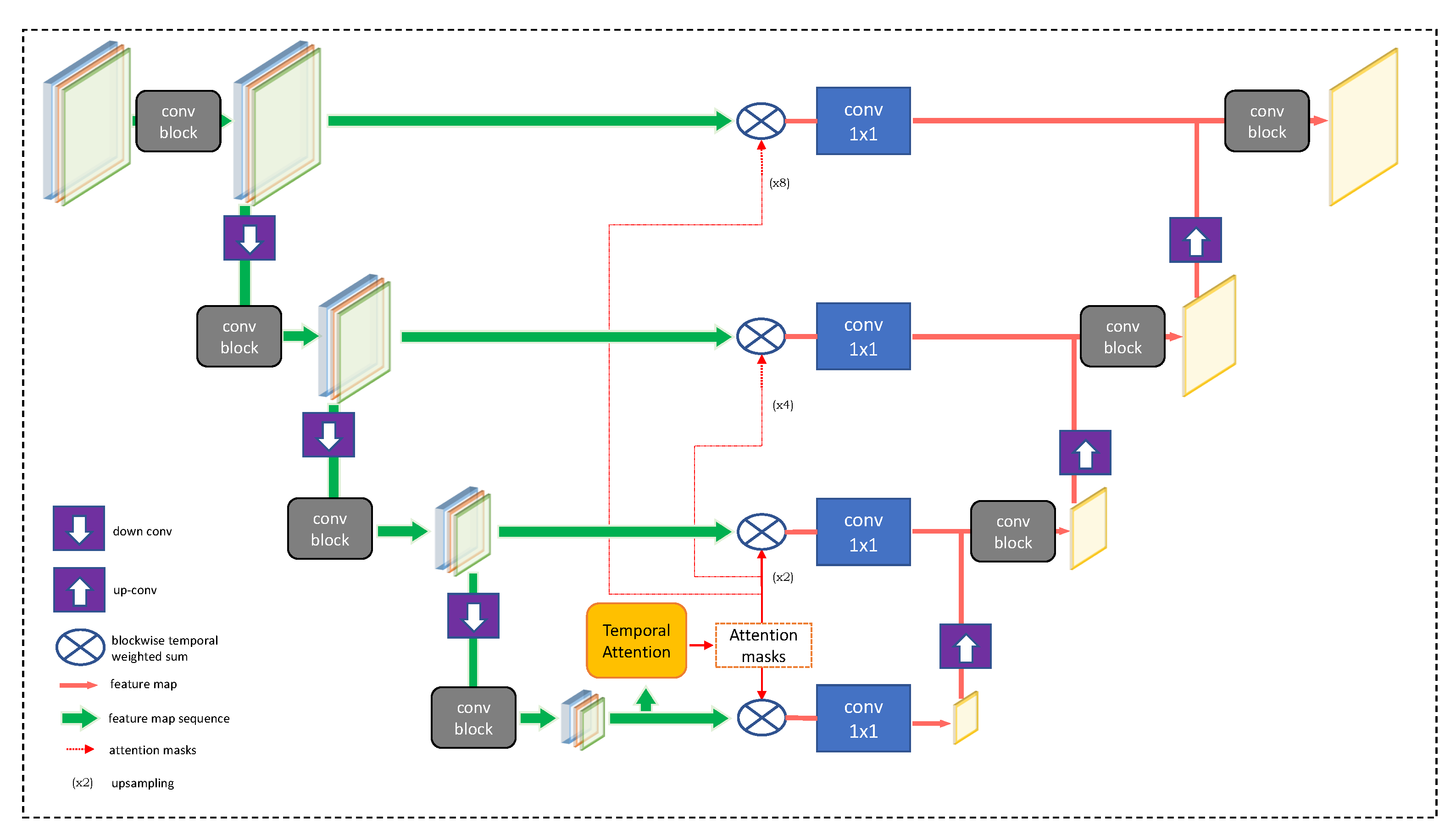
We build on the U-TAE model of Garnot and Landrieu [19] to predict water depth maps, as shown in Figure 7. The name stands for “U-net with Temporal Attention Encoder” and denotes a spatio-temporal encoder–decoder architecture originally developed for the segmentation of image sequences. It uses a combination of multi-scale spatial convolutions and temporal attention. The advantage of U-TAE is that its attention masks can extract salient and robust spatio-temporal features at different resolutions simultaneously, in contrast to other methods like convolutional and recurrent networks that only extract temporal features at the lowest and/or highest spatial resolutions only [19]. We adapt the U-TAE method to ingest an elevation map, an initial water depth map and rainfall values instead of a time series and to predict water depth after 2 h instead of semantic category labels.

Computational attention mechanisms have been studied across multiple fields including psychology, neuroscience, and more recently computer vision. They are motivated by how human visual attention selectively concentrates on relevant details while ignoring others in a complex scene. Such a mechanism can be viewed as an active adjustment of feature weights, where high attention weight corresponds to the higher importance of a feature [43,44]. The U-TAE network is composed of three components: a spatial encoder, a temporal encoder, and a spatial decoder.

The encoder follows the popular U-net [45]: multiple levels of convolution, non-linear activation and normalization encode each input layer separately into a latent representation as depicted in Figure 7. Each level halves the spatial height and width of the input.

The temporal encoder merges the information in different input maps into a singular map per scale level. In the U-TAE framework, the attention mechanism operates only on the lowest resolution feature maps; then, the same attention masks are upsampled and applied at all resolutions. Attention is implemented via the Lightweight Temporal Attention Encoder (L-TAE) network, a simplified variant of multi-head self-attention [46]. At the lowest resolution level, the L-TAE generates G temporal attention masks for each pixel of the feature map sequence. These attention masks are spatially upsampled to other encoder levels (respectively, scales) with bilinear interpolation [19].

After temporal encoding, the temporally aggregated feature maps are fed into a convolutional decoder, where each block again consists of convolutions, ReLU activations [47], and batch normalisation [48]. Each block doubles the spatial width and height of the feature maps and then appends the feature maps of the corresponding scale level, following the U-Net principle [19].

To train the model, the following loss function is minimized:

$${\mathcal{L}}_{NSE}=\frac{{\sum }_{i=1}^n{(y_i-x_i)}^2}{{\sum }_{i=1}^n{(x_i-\overline{x})}^2},$$

(1)

where $y_i$ is the predicted water depth at pixel i, $x_{i,t}$ is the simulated water depth at pixel i and $\overline{x}$ is the mean simulated water depth. The loss function is inspired by the Nash–Sutcliffe efficiency (NSE),

$$NSE=1-\frac{{\sum }_{i=1}^n{(y_i-x_i)}^2}{{\sum }_{i=1}^n{(x_i-\overline{x})}^2}.$$

(2)

The NSE was proposed by [49] and is arguably the most popular performance metric for hydrological model evaluation [50,51,52]. It can be computed as the difference between one and the absolute sum of squared residuals of simulated and predicted values, normalised by the variance of the simulated value. The NSE metric measures model performance on a scale $(-\infty ,1]$. A value of 1 indicates perfect agreement between predicted and reference water depth, and smaller values indicate lower agreement [51].

4.2. Model Training

The SwissFlood dataset is divided into distinct training and test sets. We set aside 10 ($10\%$ of the dataset) catchment areas for testing. We further allocate 18 ($20\%$ of the training set) catchments as the validation set to optimise the model performance. The validation serves to assess model skill on samples not used during the update of the model parameters in order to tune hyper-parameters of the training process. Moreover, three rainfall events are also held out from the training set to test model performance on unseen events. The input data to the model and its architecture are described in Section 4. The output is the estimated water depth predictions for every pixel in the catchment for the end of the two-hour prediction window. The boundary conditions are the same for all the catchments and they are defined as an infinite sink.

As outlined in Section 3.2, we assume spatially uniform rainfall intensity over the catchment area. To provide this information to the network, we create a 2D map with the same rainfall value at every pixel and feed those maps to the network as separate channels. We create 12 such channels $[{\mathbf{r}}_t,{\mathbf{r}}_{t+10},{\mathbf{r}}_{t+20},\cdots ,{\mathbf{r}}_{t+110}]$ for the forecasting period. Together with the elevation map and the initial water depths at time t, the model therefore receives 14 channels.

The full catchments are too large to process; therefore, we crop patches of size 256 × 256 pixels and feed those to the network. For training, the patches are sampled randomly at run-time with a batch size of 16 patches. The randomization offers greater diversity than using a fixed patch layout. Only patches with at least 10% of the pixels inside the catchment boundary are used. The network is initialised with random weights and trained by minimising the objective function as described in Equation (1). The network weights are updated with back-propagation as is common for neural networks, using the Adam [53] optimizer. We train the model for 1000 epochs, where an epoch corresponds to the number of iterations it takes for the model to go through the complete training set. The base learning rate is set to $0.0001$. We use L-TAE with 4 heads for temporal encoding. As is common in deep learning applications, these hyper-parameter settings were chosen based on performance on the validation set.

5. Results

In this section, we present the results obtained by our model, i.e., its skill in predicting the water depth two hours in advance.

In addition to the U-TAE model, we also run a simpler convolutional neural network (CNN) with three convolution+activation layers as a baseline approach. That baseline receives the same inputs and is trained with L1, L2 and ${\mathcal{L}}_{NSE}$ loss functions. From now on, we refer to the CNN model trained with L1 loss as Baseline-1, and to the CNN model trained with L2 loss as Baseline-2. The CNN trained with ${\mathcal{L}}_{NSE}$ loss will be labelled as Baseline-3. The L1 and L2 loss functions are defined as the mean absolute, respectively, squared, prediction residuals:

$$L1=\sum _{i=1}^n|\overline{y_i}-y_i|,$$

(3)

$$L2=\sum _{i=1}^n{(\overline{y_i}-y_i)}^2$$

(4)

where $\overline{y_i}$ denotes the model prediction of and $y_i$ the target value.

As outlined in Section 3, we have a total of one hundred catchments in our SwissFlood dataset, divided into 72 training, 18 validation, and 10 test catchments, see Section 4.2. The CADDIES simulations were performed with 15 different rainfall events for each catchment. For the 72 catchments in the training set, we hold out three rainfall events for evaluation. We call this set seen, as the model does not know the rainfall event but has seen the topography of the catchment while training. The 10 catchment areas which the model has never seen during training and validation are termed unseen. As previously stated all rainfall events used in the study are unique, i.e., the same event has never been applied to different catchments.

To evaluate the performance of our U-TAE model, we compare the resulting water depth maps to those produced by the CADDIES flood model and generate quantitative performance metrics as shown in

Table 1. Mean absolute errors of our model (in centimetres) averaged over all rainfall events, across different ranges of water depth.

		Mean Absolute Errors (cm)
		all	≥5	≥10	≥20	≥50	≥100
Baseline-1	unseen	1.61	28.29	46.75	67.54	97.37	117.82
	seen	1.45	21.15	35.51	54.87	86.60	105.35
Baseline-2	unseen	2.40	27.33	44.41	63.51	91.65	112.05
	seen	2.07	20.28	33.53	51.34	81.55	100.25
Baseline-3	unseen	2.35	27.91	46.09	66.65	96.78	117.85
	seen	2.05	20.70	34.90	54.05	86.18	105.74
Ours	unseen	1.18	17.99	28.99	40.79	57.06	67.76
	seen	0.75	7.50	11.81	16.72	23.59	26.86

. As a metric, we use the widely used and easily interpretable mean absolute error (MAE), defined as:

$$MAE=\frac{1}{N}\sum _{i=1}^N|\overline{y_{i,t}}-y_{i,t}|,$$

(5)

where $\overline{y_{i,t}}$ denotes the model prediction and $y_{i,t}$ is the target value. A value of zero indicates a perfect fit and the error values have the same unit as our target values. We analyse the predicted water depth results across a range of different depth intervals to obtain a more comprehensive picture of model performance.

We report the results in six different ranges which are as follows: pixels with water depth ≥5, ≥10, ≥20, ≥50, ≥100, and all pixels. Table 1 summarises the quantitative results for our model and the baselines, for both the seen and unseen test sets. The table confirms that our approach outperforms all three baselines. Moreover, the performance of our model on the seen test set is much better than on the unseen one, suggesting that the deep learning model can handle new rainfall events more effectively when it has already seen the catchment topography before. The MAE for higher ranges ≥20, ≥50, and ≥100 is more than 50% higher in the unseen setting. Regardless of the test set, MAE values with our approach have acceptable magnitudes, in agreement with previous research [14,33]. Especially for seen catchments, the prediction performance is rather good, but even when generalizing to unseen regions, there is a significant improvement over the baselines. For all three models—Baseline-1, Baseline-2 and Baseline-3—it is evident that there is only a slight improvement from unseen to seen locations. This suggests that the baseline models have not managed to learn location-specific patterns.

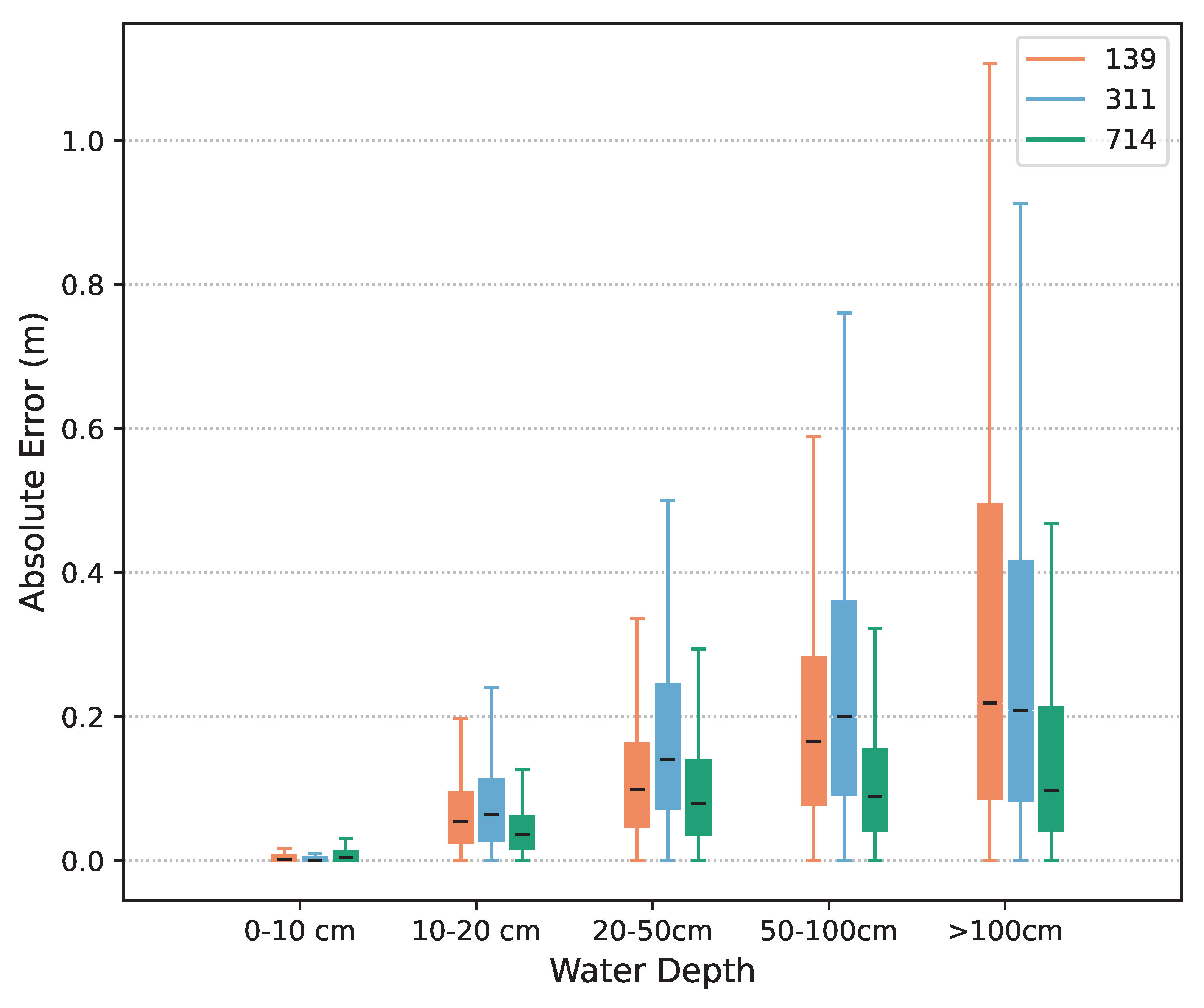
To complement the quantitative evaluation in Table 1, we also present the qualitative results of our model. Figure 8 shows a box plot, with binned water depth ranges on the x-axis and absolute errors on the y-axis. We show the results for three representative catchments from the test set. Overall, we observe a low absolute error value in shallow water depths that increases as we move to deeper water. For catchments 139 (minimum elevation 708 m, maximum elevation 1429 m, area 5.72 km²) and 311 (minimum elevation 468 m, maximum elevation 2690 m, area 10.06 km²), we observe an increase in absolute error across all levels except 0–10 cm. In more detail, median errors actually remain low, but the worst predictions, at only a few pixels, are increasingly further off as the water depth increases. Catchments 139 and 311 experienced significantly deeper simulated water depth compared to catchment 714. Catchment 139 had a maximum depth of 13.21 m for rainfall event tr35_135, which peaked at around 65 mm/h with two smaller peaks of 40 mm/h at the beginning and end of the event. Catchment 311 reached a maximum depth of 15.06 m for event tr20_57, with a peak of 20 mm/h lasting approximately 15 min. In contrast, catchment 714, with an elevation range of 399 m to 831 m and an area of 9.27 km², only reached a maximum depth of 6.6 m for event tr35_367. This event had no distinct peak but rather near-constant rainfall, contributing to overall higher absolute errors in catchments 139 and 311.

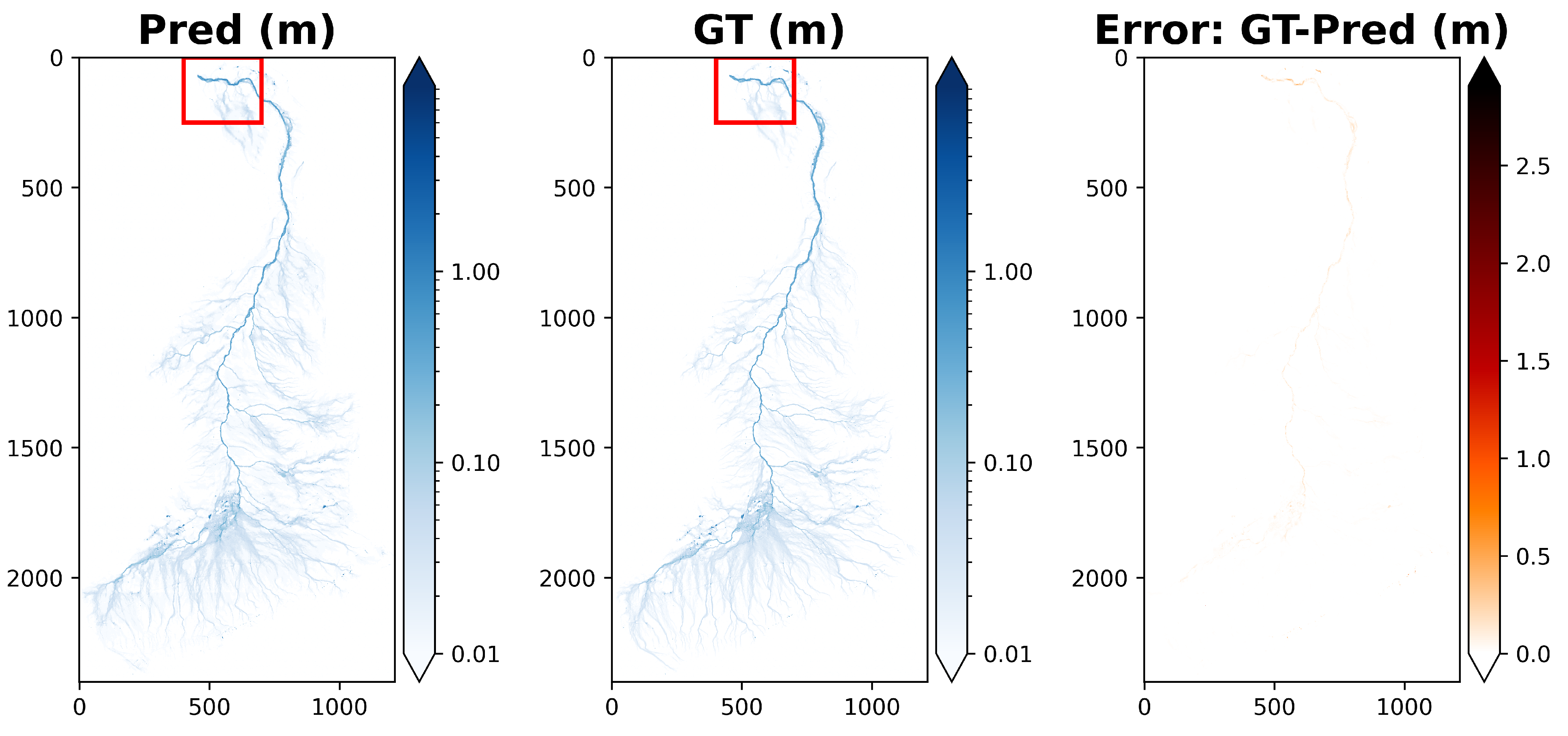
In Figure 9, Figure 10, Figure 11 and Figure 12, we show an example of the qualitative performance of our model. Figure 9 depicts the complete reconstruction of catchment 127 for rainfall event tr35_161 and a timestep of 190 min. The red bounding box is shown magnified in Figure 10. A visual analysis of the figures suggests that the water depth predictions of the model are reasonably accurate. The rightmost plot shows the absolute residual errors between ground truth and prediction. Here, a darker colour corresponds to a higher error. We zoom into regions with particularly high errors in Figure 10. In the top right corner, marked by a yellow bounding box, the extent of a high water depth area has been underestimated by the model. We also see a mild smoothing effect in the green bounding box. Figure 10 shows lower absolute errors compared to Figure 9, implying the presence of isolated pixels with high error, as previously observed in the box plot figure. Similarly, Figure 11 shows another reconstruction, for catchment 151, with high water depth values. When we zoom into the patch area in Figure 12, we observe a fuzzy border around the high water depth area in the yellow bounding box instead of sharp water depth changes. As suggested by the quantitative results, absolute error is positively correlated with water depth, i.e., errors are larger for deeper water.

Ablation Studies

To train a deep neural network, one minimizes a loss function [54]. It is therefore critical to find a loss function that aligns well with the intended model behaviour. In this section, we study the impact of different loss functions on the predictive skill of our approach. Specifically, we compare our NSE loss (Equation (1)) with the most common loss functions for regression tasks, namely the L1 and L2 losses as given in Equations (3) and (4). For computational efficiency, the three variants are trained and validated only on a subset of catchments from the Swissflood dataset, while the test set of unseen catchments remains the same. We report the results for different water depth ranges in

Table 2. Mean absolute errors of our model (in centimetres) on test data, with different loss functions used for training.

		Mean Absolute Errors (cm)
		All	≥5	≥10	≥20	≥50	≥100
NSE	unseen	1.56	23.16	37.49	53.61	78.09	97.58
L1	unseen	1.47	24.7	40.53	58.46	85.02	106.03
L2	unseen	1.70	24.6	39.47	56.74	83.93	105.55

. One can see that the NSE loss performs better than the L2 loss function for all water depth ranges. The L1 loss performs similarly to the NSE loss overall (in fact even marginally better), but this is entirely due to a slightly lower error at very low water depths between 0 and 5 cm, presumably due to the well-established tendency of L1 to drive very low values to exactly 0. At all water depths ≥5 cm, NSE still prevails.

6. Discussion and Conclusions

A large body of literature exists about flood prediction and management strategies [55]. Some recent works [5,34] have explored deep learning for flood forecasting and prediction as described in Section 2. Seleem et al. [34] use multiple predictive features, including topographical elements derived from the digital elevation model. Similarly, Löwe et al. [5] and Guo et al. [14] have also defined varying numbers of such features to help a neural network learn the dynamics of water movement over terrain. In contrast to these works, our approach requires only three inputs to predict water depth with a lead time of 120 min: a DEM of the catchment, rainfall values, and the pixel-wise water depth at the starting time. Unlike previous research [14], we have also evaluated model performance thoroughly both in the setting of unseen rainfall in seen catchments and in the more challenging setting of unseen rainfall in unseen catchments. The results demonstrate that our model, as expected, works better in the former case but also generalizes quite well to the latter. As far as we are aware, our research is one of the first data-driven works to demonstrate high-resolution, spatially explicit flood depth prediction for previously unobserved rainfall events and/or catchments.

When compared to the physically grounded flood model, our data-driven technique eliminates the need for exhaustive manual fine-tuning for every individual scene and rain event, which can be challenging and time-consuming in practice. While the physically based flood model requires expertise in hydrology and the catchment specifications, our model only uses a standard rainfall forecast and a digital elevation model of the area under study. We acknowledge that there are other factors such as land use patterns, infrastructures, soil characteristics, backwater effects, and storm water systems that can influence flood predictions. Building upon the work presented in the present paper, the methodology can be improved by including these additional factors. This would ideally offer a more detailed representation of urban flood dynamics and can be incorporated as new input layers to the model in addition to the DEM and rainfall values. We hypothesise that integrating these additional data, once they become available at a large scale, would likely improve the performance of our model in simulating urban inundations.

6.1. Limitations of the Proposed Approach

In our work, we estimate water depth for a two-hour lead time (e.g., to inform an early warning system). However, for a different lead time requirement, the model would need to be re-trained. A possible direction for future work could be to design a network that gives multiple outputs associated with different lead times. Figure 8, Figure 9, Figure 10 and Figure 11 show high absolute errors for very deep water. We hypothesise that the underlying reason is the very small number of training samples with such large water depths, which leads the global loss function to focus on shallower regions. This limitation can be addressed in future work by designing a loss function that puts more weight on large depth values, or by collecting more data that includes many large depth values. We assume in our work spatially uniform rainfall over the catchment area, which could be addressed in future works by integrating spatially variable rainfall which can more accurately capture precipitation variability. Because our model was trained on simulations from the CADDIES flood model, its performance is implicitly bounded by that simulator. CADDIES only approximates the true, underlying physical principles and we used it to generate our dataset because we found it to be reasonably computationally efficient. Our analysis is strongly dependent on the simulated data. Furthermore, an independent validation of the accuracy of the CADDIES 2D model with reference data collected in situ is not feasible for our large data set. Lastly, deep learning models excel at accurately fitting to observational data and have a proven ability to emulate physical principles within the data distribution. However, when encountering inputs that considerably diverge from the training dataset, data-driven models may generate physically inconsistent or implausible predictions, due to extrapolation or observational biases [56,57,58]. This can cause a considerable degradation in performance, a limitation not present in physics-based hydrodynamic models.

6.2. Conclusions

We have presented a novel method for predicting high-resolution water depth maps with a two-hour lead time for urban pluvial flooding. We use a deep learning network with sequence encoding and temporal attention to forecast future water depths based on elevation data, current water depths, and precipitation forecasts. For our study, we have moreover introduced the SwissFlood dataset, which includes simulations for 100 Swiss catchments and 1500 rainfall events extracted from real observations.

We have trained the proposed model on the SwissFlood dataset and have compared it with simulation outcomes from CADDIES, hydrodynamic flood model. We demonstrate that the trained model can predict water depth maps with fair accuracy and that it is capable of generalizing to unseen rainfall events and unseen catchments. The mean absolute error remains as low as 27 cm even in instances of severe flooding with water depths surpassing 1 m. Ablation studies with different loss functions confirmed that the Nash–Sutcliffe efficiency (NSE) as a loss function outperforms L1 and L2 loss functions for higher water depth ranges. We hope to have shown that attention-based neural models can be a promising tool for future pluvial flood alert systems.

References

1. do Lago, C.A.; Giacomoni, M.H.; Bentivoglio, R.; Taormina, R.; Gomes, M.N.; Mendiondo, E.M. Generalizing rapid flood predictions to unseen urban catchments with conditional generative adversarial networks. J. Hydrol. 2023, 618, 129276. [Google Scholar] [CrossRef]
2. UNESCO. World Water Assessment Programme. In The United Nations World Water Development Report 2020: Water and Climate Change; UNESCO: Paris, France, 2020. [Google Scholar]
3. Bhola, P.K.; Leandro, J.; Disse, M. Framework for Offline Flood Inundation Forecasts for Two-Dimensional Hydrodynamic Models. Geosciences 2018, 8, 346. [Google Scholar] [CrossRef]
4. Kabir, S.; Patidar, S.; Xia, X.; Liang, Q.; Neal, J.; Pender, G. A deep convolutional neural network model for rapid prediction of fluvial flood inundation. J. Hydrol. 2020, 590, 125481. [Google Scholar] [CrossRef]
5. Löwe, R.; Böhm, J.; Jensen, D.G.; Leandro, J.; Rasmussen, S.H. U-FLOOD–Topographic deep learning for predicting urban pluvial flood water depth. J. Hydrol. 2021, 603, 126898. [Google Scholar] [CrossRef]
6. Hu, R.; Fang, F.; Pain, C.; Navon, I. Rapid spatio-temporal flood prediction and uncertainty quantification using a deep learning method. J. Hydrol. 2019, 575, 911–920. [Google Scholar] [CrossRef]
7. Berkhahn, S.; Fuchs, L.; Neuweiler, I. An ensemble neural network model for real-time prediction of urban floods. J. Hydrol. 2019, 575, 743–754. [Google Scholar] [CrossRef]
8. Guo, Z.; Leitão, J.P.; Simões, N.E.; Moosavi, V. Data-driven flood emulation: Speeding up urban flood predictions by deep convolutional neural networks. J. Flood Risk Manag. 2021, 14, e12684. [Google Scholar] [CrossRef]
9. Xie, S.; Wu, W.; Mooser, S.; Wang, Q.; Nathan, R.; Huang, Y. Artificial neural network based hybrid modeling approach for flood inundation modeling. J. Hydrol. 2021, 592, 125605. [Google Scholar] [CrossRef]
10. Yokoya, N.; Yamanoi, K.; He, W.; Baier, G.; Adriano, B.; Miura, H.; Oishi, S. Breaking Limits of Remote Sensing by Deep Learning From Simulated Data for Flood and Debris-Flow Mapping. IEEE Trans. Geosci. Remote Sens. 2022, 60, 1–15. [Google Scholar] [CrossRef]
11. Zhao, G.; Pang, B.; Xu, Z.; Cui, L.; Wang, J.; Zuo, D.; Peng, D. Improving urban flood susceptibility mapping using transfer learning. J. Hydrol. 2021, 602, 126777. [Google Scholar] [CrossRef]
12. LeCun, Y.; Bengio, Y.; Hinton, G. Deep learning. Nature 2015, 521, 436. [Google Scholar] [CrossRef] [PubMed]
13. Bengio, Y.; Courville, A.; Vincent, P. Representation Learning: A Review and New Perspectives. IEEE Trans. Pattern Anal. Mach. Intell. 2013, 35, 1798–1828. [Google Scholar] [CrossRef] [PubMed]
14. Guo, Z.; Moosavi, V.; Leitão, J.P. Data-driven rapid flood prediction mapping with catchment generalizability. J. Hydrol. 2022, 609, 127726. [Google Scholar] [CrossRef]
15. Lin, Q.; Leandro, J.; Wu, W.; Bhola, P.; Disse, M. Prediction of Maximum Flood Inundation Extents with Resilient Backpropagation Neural Network: Case Study of Kulmbach. Front. Earth Sci. 2020, 8, 332. [Google Scholar] [CrossRef]
16. Zhou, Y.; Wu, W.; Nathan, R.; Wang, Q.J. A rapid flood inundation modelling framework using deep learning with spatial reduction and reconstruction. Environ. Model. Softw. 2021, 143, 105112. [Google Scholar] [CrossRef]
17. Guidolin, M.; Chen, A.S.; Ghimire, B.; Keedwell, E.C.; Djordjević, S.; Savić, D.A. A weighted cellular automata 2D inundation model for rapid flood analysis. Environ. Model. Softw. 2016, 84, 378–394. [Google Scholar] [CrossRef]
18. MeteoSwiss. Federal Office for Meteorology and Climatology. 2023. Available online: https://www.meteoswiss.admin.ch/ (accessed on 17 January 2024).
19. Garnot, V.S.F.; Landrieu, L. Panoptic Segmentation of Satellite Image Time Series With Convolutional Temporal Attention Networks. In Proceedings of the IEEE/CVF International Conference on Computer Vision (ICCV), Montreal, QC, Canada, 11–17 October 2021; pp. 4872–4881. [Google Scholar]
20. Jafarzadegan, K.; Abbaszadeh, P.; Moradkhani, H. Sequential data assimilation for real-time probabilistic flood inundation mapping. Hydrol. Earth Syst. Sci. 2021, 25, 4995–5011. [Google Scholar] [CrossRef]
21. Bentivoglio, R.; Isufi, E.; Jonkman, S.N.; Taormina, R. Deep learning methods for flood mapping: A review of existing applications and future research directions. Hydrol. Earth Syst. Sci. 2022, 26, 4345–4378. [Google Scholar] [CrossRef]
22. Wang, Y.; Karimi, H.A. Impact of spatial distribution information of rainfall in runoff simulation using deep learning method. Hydrol. Earth Syst. Sci. 2022, 26, 2387–2403. [Google Scholar] [CrossRef]
23. Solomatine, D.P.; Ostfeld, A. Data-driven modelling: Some past experiences and new approaches. J. Hydroinform. 2008, 10, 3–22. [Google Scholar] [CrossRef]
24. Kröhnert, M.; Eltner, A. Versatile Mobile and Stationary Low-Cost Approaches for Hydrological Measurements. Int. Arch. Photogramm. Remote Sens. Spat. Inf. Sci. 2018, XLII-2, 543–550. [Google Scholar] [CrossRef]
25. Ning, H.; Li, Z.; Hodgson, M.E.; Wang, C.S. Prototyping a Social Media Flooding Photo Screening System Based on Deep Learning. ISPRS Int. J. Geo-Inf. 2020, 9, 104. [Google Scholar] [CrossRef]
26. Chaudhary, P.; D’Aronco, S.; Moy de Vitry, M.; Leitão, J.P.; Wegner, J.D. Flood-Water Level Estimation from Social Media Images. ISPRS Ann. Photogramm. Remote Sens. Spat. Inf. Sci. 2019, IV-2/W5, 5–12. [Google Scholar] [CrossRef]
27. Chaudhary, P.; D’Aronco, S.; Leitão, J.; Schindler, K.; Wegner, J. Water level prediction from social media images with a multi-task ranking approach. ISPRS J. Photogramm. Remote Sens. 2020, 167, 252–262. [Google Scholar] [CrossRef]
28. Quan, K.A.C.; Nguyen, V.T.; Nguyen, T.C.; Nguyen, T.V.; Tran, M.T. Flood Level Prediction via Human Pose Estimation from Social Media Images. In Proceedings of the 2020 International Conference on Multimedia Retrieval, ICMR ’20, New York, NY, USA, 8–11 June 2020; pp. 479–485. [Google Scholar]
29. Moy de Vitry, M.; Kramer, S.; Wegner, J.D.; Leitão, J.P. Scalable flood level trend monitoring with surveillance cameras using a deep convolutional neural network. Hydrol. Earth Syst. Sci. 2019, 23, 4621–4634. [Google Scholar] [CrossRef]
30. Lütjens, B.; Leshchinskiy, B.; Requena-Mesa, C.; Chishtie, F.; Rodríguez, N.D.; Boulais, O.; Piña, A.; Newman, D.; Lavin, A.; Gal, Y.; et al. Physics-informed GANs for Coastal Flood Visualization. arXiv 2020, arXiv:2010.08103. [Google Scholar]
31. Lütjens, B.; Leshchinskiy, B.; Requena-Mesa, C.; Chishtie, F.; Rodríguez, N.D.; Boulais, O.; Sankaranarayanan, A.; Piña, A.; Gal, Y.; Raïssi, C.; et al. Physically Consistent Generative Adversarial Networks for Coastal Flood Visualization. arXiv 2021, arXiv:2104.04785. [Google Scholar]
32. Bowes, B.D.; Tavakoli, A.; Wang, C.; Heydarian, A.; Behl, M.; Beling, P.A.; Goodall, J.L. Flood mitigation in coastal urban catchments using real-time stormwater infrastructure control and reinforcement learning. J. Hydroinform. 2020, 23, 529–547. [Google Scholar] [CrossRef]
33. Chaudhary, P.; Leitão, J.P.; Donauer, T.; D’Aronco, S.; Perraudin, N.; Obozinski, G.; Perez-Cruz, F.; Schindler, K.; Wegner, J.D.; Russo, S. Flood Uncertainty Estimation Using Deep Ensembles. Water 2022, 14, 2980. [Google Scholar] [CrossRef]
34. Seleem, O.; Ayzel, G.; Bronstert, A.; Heistermann, M. Transferability of data-driven models to predict urban pluvial flood water depth in Berlin, Germany. Nat. Hazards Earth Syst. Sci. 2023, 23, 809–822. [Google Scholar] [CrossRef]
35. Ivanov, V.Y.; Xu, D.; Dwelle, M.C.; Sargsyan, K.; Wright, D.B.; Katopodes, N.; Kim, J.; Tran, V.N.; Warnock, A.; Fatichi, S.; et al. Breaking Down the Computational Barriers to Real-Time Urban Flood Forecasting. Geophys. Res. Lett. 2021, 48, e2021GL093585. [Google Scholar] [CrossRef]
36. Tran, H.; Leonarduzzi, E.; De la Fuente, L.; Hull, R.B.; Bansal, V.; Chennault, C.; Gentine, P.; Melchior, P.; Condon, L.E.; Maxwell, R.M. Development of a Deep Learning Emulator for a Distributed Groundwater-Surface Water Model: ParFlow-ML. Water 2021, 13, 3393. [Google Scholar] [CrossRef]
37. Muñoz, D.F.; Muñoz, P.; Moftakhari, H.; Moradkhani, H. From local to regional compound flood mapping with deep learning and data fusion techniques. Sci. Total. Environ. 2021, 782, 146927. [Google Scholar] [CrossRef]
38. Kao, I.F.; Liou, J.Y.; Lee, M.H.; Chang, F.J. Fusing stacked autoencoder and long short-term memory for regional multistep-ahead flood inundation forecasts. J. Hydrol. 2021, 598, 126371. [Google Scholar] [CrossRef]
39. Chang, D.L.; Yang, S.H.; Hsieh, S.L.; Wang, H.J.; Yeh, K.C. Artificial Intelligence Methodologies Applied to Prompt Pluvial Flood Estimation and Prediction. Water 2020, 12, 3552. [Google Scholar] [CrossRef]
40. Lin, Q.; Leandro, J.; Gerber, S.; Disse, M. Multistep Flood Inundation Forecasts with Resilient Backpropagation Neural Networks: Kulmbach Case Study. Water 2020, 12, 3568. [Google Scholar] [CrossRef]
41. Zahura, F.T.; Goodall, J.L.; Sadler, J.M.; Shen, Y.; Morsy, M.M.; Behl, M. Training Machine Learning Surrogate Models from a High-Fidelity Physics-Based Model: Application for Real-Time Street-Scale Flood Prediction in an Urban Coastal Community. Water Resour. Res. 2020, 56, e2019WR027038. [Google Scholar] [CrossRef]
42. Ghimire, B.; Chen, A.S.; Guidolin, M.; Keedwell, E.C.; Djordjević, S.; Savić, D.A. Formulation of a fast 2D urban pluvial flood model using a cellular automata approach. J. Hydroinform. 2012, 15, 676–686. [Google Scholar] [CrossRef]
43. Guo, M.H.; Xu, T.X.; Liu, J.J.; Liu, Z.N.; Jiang, P.T.; Mu, T.J.; Zhang, S.H.; Martin, R.R.; Cheng, M.M.; Hu, S.M. Attention mechanisms in computer vision: A survey. Comput. Vis. Media 2022, 8, 331–368. [Google Scholar] [CrossRef]
44. Yang, X. An Overview of the Attention Mechanisms in Computer Vision. J. Physics Conf. Ser. 2020, 1693, 012173. [Google Scholar] [CrossRef]
45. Ronneberger, O.; Fischer, P.; Brox, T. U-Net: Convolutional Networks for Biomedical Image Segmentation. In Proceedings of the Medical Image Computing and Computer-Assisted Intervention–MICCAI 2015, Munich, Germany, 5–9 October 2015; pp. 234–241. [Google Scholar]
46. Garnot, V.S.F.; Landrieu, L. Lightweight Temporal Self-Attention for Classifying Satellite Image Time Series. In Proceedings of the Advanced Analytics and Learning on Temporal Data: 5th ECML PKDD Workshop, AALTD 2020, Ghent, Belgium, 18 September 2020. [Google Scholar]
47. Agarap, A.F. Deep Learning using Rectified Linear Units (ReLU). arXiv 2018, arXiv:1803.08375. [Google Scholar]
48. Ioffe, S.; Szegedy, C. Batch Normalization: Accelerating Deep Network Training by Reducing Internal Covariate Shift. In Proceedings of the 32nd International Conference on Machine Learning, Lille, France, 1 June 2015; Volume 37, pp. 448–456. [Google Scholar]
49. Nash, J.; Sutcliffe, J. River flow forecasting through conceptual models part I—A discussion of principles. J. Hydrol. 1970, 10, 282–290. [Google Scholar] [CrossRef]
50. Shalev, G.; El-Yaniv, R.; Klotz, D.; Kratzert, F.; Metzger, A.; Nevo, S. Accurate Hydrologic Modeling Using Less Information. arXiv 2019, arXiv:1911.09427. [Google Scholar]
51. Krause, P.; Boyle, D.; Bäse, F. Comparison of different efficiency criteria for hydrological model assessment. Adv. Geosci. 2005, 5, 89–97. [Google Scholar] [CrossRef]
52. Gupta, H.V.; Kling, H.; Yilmaz, K.K.; Martinez, G.F. Decomposition of the mean squared error and NSE performance criteria: Implications for improving hydrological modelling. J. Hydrol. 2009, 377, 80–91. [Google Scholar] [CrossRef]
53. Kingma, D.P.; Ba, J. Adam: A method for stochastic optimization. In Proceedings of the International Conference on Learning Representations (ICLR), San Diego, CA, USA, 7–9 May 2015. [Google Scholar]
54. Ciampiconi, L.; Elwood, A.; Leonardi, M.; Mohamed, A.; Rozza, A. A survey and taxonomy of loss functions in machine learning. arXiv 2023, arXiv:2301.05579. [Google Scholar]
55. Pugliese, R.; Regondi, S.; Marini, R. Machine learning-based approach: Global trends, research directions, and regulatory standpoints. Data Sci. Manag. 2021, 4, 19–29. [Google Scholar] [CrossRef]
56. Reichstein, M.; Camps-Valls, G.; Stevens, B.; Jung, M.; Denzler, J.; Carvalhais, N.; Prabhat. Deep learning and process understanding for data-driven Earth system science. Nature 2019, 566, 195–204. [Google Scholar] [CrossRef] [PubMed]
57. Cortés-Andrés, J.; Camps-Valls, G.; Sippel, S.; Székely, E.; Sejdinovic, D.; Diaz, E.; Pérez-Suay, A.; Li, Z.; Mahecha, M.; Reichstein, M. Physics-aware nonparametric regression models for Earth data analysis. Environ. Res. Lett. 2022, 17, 054034. [Google Scholar] [CrossRef]
58. Marcus, G.F. Deep Learning: A Critical Appraisal. arXiv 2018, arXiv:1801.00631. [Google Scholar]
Figure 1. The flowchart of our entire workflow from data collection to water depth predictions with a two-hour lead time.
Water 16 01286 g001
Figure 2. Location of Swissflood catchments, colour-coded to denote the training, validation and test sets.
Water 16 01286 g002
Figure 3. Overview of SwissFlood catchment properties: maximum slope, mean slope, elevation difference, and area of the catchments.
Water 16 01286 g003
Figure 4. Illustration of hyetographs used for simulations. The name of the event is given in the upper right corner. Examples are taken from the training (top row), validation (middle row) and test sets (bottom row).
Water 16 01286 g004
Figure 5. Distribution of water depth values within catchment 809 when simulating rainfall event tr35_343.
Water 16 01286 g005
Figure 6. The overview of our deep learning approach. The model receives as input the digital elevation model (DEM), current water depth, and rainfall values for the forecast period. The output consists of a pixel-wise water depth estimation across the DEM with a two-hour lead time.
Water 16 01286 g006
Figure 7. The network architecture of U-TAE as used in this paper.
Water 16 01286 g007
Figure 8. Predicted water depths and corresponding absolute errors, shown as a box plot. The predictions are provided for our model tested on catchments 139, 311, and 714, with rainfall events tr35_135, tr20_57 and tr35_367, respectively.
Water 16 01286 g008
Figure 9. On the left are the water depths predicted by our model for the complete catchment 127 at at a specific time step of rainfall event tr35_161. In the middle are the ground truth water depths. On the right is the absolute error between ground truth and prediction.
Water 16 01286 g009
Figure 10. Zoom into the region marked in Figure 9. On the left is the model prediction; in the middle is the ground truth; on the right is the absolute deviation between ground truth and prediction.
Water 16 01286 g010
Figure 11. On the left are the water depths predicted by our method for the complete catchment 151 at a specific time step of rainfall event tr35_719. In the middle are the ground truth water depths. On the right is the absolute error between ground truth and prediction.
Water 16 01286 g011
Figure 12. Zoom into the region marked in Figure 11. On the left is the model prediction; in the middle is the ground truth; on the right is the absolute deviation between ground truth and prediction. Note the fuzzy border around a pronounced depth change.
Water 16 01286 g012