1. Introduction
The availability of water resources at regional or local levels are strictly related to the precipitation rates at these scales. At the same time, there is some evidence that the recent climate change affected precipitation, at least in its globally evaluated mean values, or with reference to latitude [
1].
At present, Global Climate Models (GCMs) and Regional Climate Models (RCMs) are the main tools for simulating the behavior of the climate system. By means of these dynamical models, one is able to perform attribution studies by investigating the major (natural or anthropogenic) external forcings that influence the mean values of some meteo-climatic variables, such as temperature or precipitation.
However, when passing from global to regional scales, these models do not allow us to reconstruct and attribute precipitation changes in a very satisfying manner. This is quite understandable because, at this scale, the enhanced interannual variability can mask any direct link between global forcings and precipitation. Thus, in this situation, a more direct influence on precipitation changes at regional and local scales can be found in the behavior of certain circulation patterns, by considering some indices, their phases, and regimes. Recently, many studies analyzed these links in several regions of the world. The case of the influence of the opposite phases of the North Atlantic Oscillation (NAO) on the winter climate in Europe is well known: see, for instance [
2].
In this framework, it is quite reasonable to think of a complete attribution at regional scale as a two-step problem, which requires the identification of the influence of external forcings on circulation patterns and their regimes (first step), and the linking of these patterns with the main climatic variables at this scale (second step). The first part of this problem has been extensively investigated in the past (see [
3] for a pioneering study, and [
4] for a more recent analysis, with models forced by Sea Surface Temperatures—SSTs). Probably, GCMs and RCMs have not yet shown a satisfying ability in simulating the behavior of these patterns during the last decades, at least if they are fed uniquely by external forcings, even if recent results are very promising [
5].
However, here we deal with the second step of this attribution problem. In particular, a case study related to a period of 50 recent years in an extended Italian Alpine area is considered. We try to understand by which circulation patterns one is able to reconstruct mean annual and seasonal precipitation values in this region. In doing so, we apply neural network (NN) modeling as a tool which permits one to achieve fully nonlinear relationships between circulation patterns and the precipitation itself.
NN modeling has already shown its validity in complementing attribution investigations performed by dynamical models on a global scale: this approach corroborates the results obtained by GCMs about the fundamental importance of anthropogenic forcings as far as the attribution of the recent global warming is concerned (see [
6,
7] for a discussion of the NN alternative approach to attribution studies and for details about results). Here, we apply this strategy of investigation to a variable (precipitation) and a scale for which, at present, a complete dynamical treatment appears more difficult and shows more severe drawbacks and limitations.
In what follows, we will briefly describe the data set (
Section 2) and an NN tool developed during the last years (
Section 3). Then, after some preliminary indications obtained in terms of bivariate linear and nonlinear analyses, the NN modeling will be applied in order to assess which combination of patterns leads to the best reconstruction results for precipitation (
Section 4). Finally, brief conclusions will be drawn and prospects of further study will be envisaged in the last section.
3. An NN Tool for Environmental Applications
An NN tool for both diagnostic characterization and forecast in complex systems has been developed some years ago [
11]. Since that date, it has been applied to diagnostic and prognostic problems in the boundary layer [
11,
12,
13,
14], and more recently, to the analysis of data and models of climatic relevance [
6,
7,
15,
16].
The kernel of this tool has been extensively described elsewhere: see [
11] for the main model and [
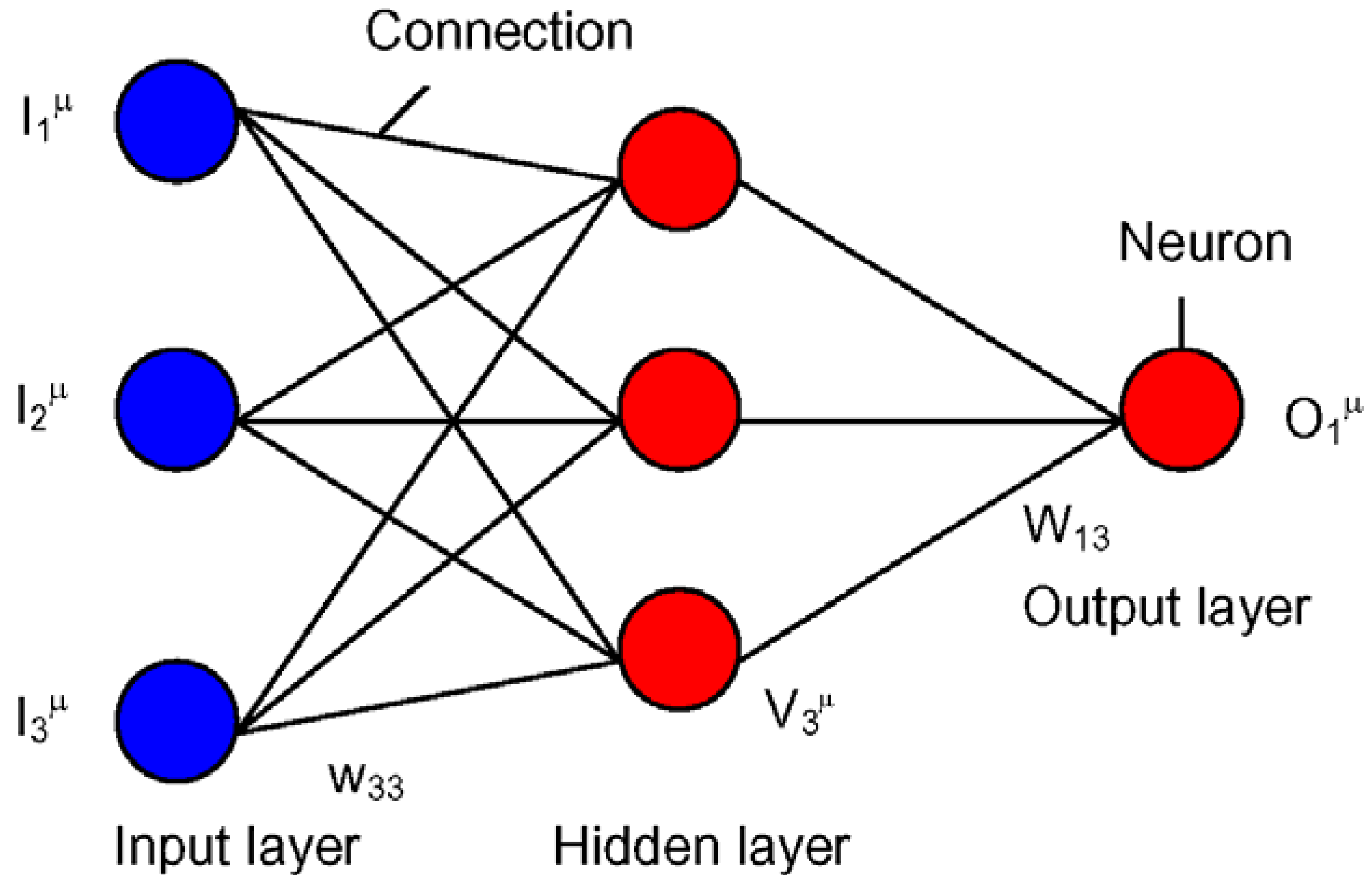
12] for a modified version of it. Here, we limit to only mention that the NNs adopted in the present investigation are feed-forward networks with one hidden layer and just a single output (see
Figure 2). Additionally, the transfer functions calculated at each neuron are sigmoids for the hidden layer and sigmoids or linear functions for the output layer. In these networks, the learning from data is performed through an error-backpropagation training characterized by generalized Widrow-Hoff rules for updating the connection weights at each iteration step
t. These rules, endowed with gradient descent and momentum terms, read as follows:
Here, with reference to the terminology also introduced in
Figure. 2,
μ (= 1, …, 49) is the number of a specific pattern of inputs-target couples,
are the targets,
i.e., the real values of data to be reconstructed by the NN,
are the outputs,
i.e., the results of the NN in reconstructing the targets,
and
are the weighted sums converging to the neurons of the hidden and output layers, respectively,
are the sigmoids calculated at hidden neurons and
are the sigmoids or linear functions calculated at the output neuron,
represent what exits from the hidden neurons after the calculation of their nonlinear transfer functions,
are the derivatives of the transfer functions,
is the learning rate, which is directly associated with the minimization of the total error (a quadratic cost function of
and
on the training set via gradient descent, and the
-term is the so called momentum term, useful for avoiding large oscillations in the learning process. A good combination of
and
permits one to escape from the relative minima of the cost function and to reach a deeper minimum.
Once the weights are fixed at the end of the iterative training (on a training set), the network becomes nothing more than a function that maps input values to output ones. However, due to the nonlinear nature of an NN regression, a neural model would be able to exactly mimic the target values without extracting any realistic regression law if the correspondent inputs-target patterns are included in the training set and a sufficiently large number of hidden neurons are allowed. Thus, first we consider few hidden neurons; second, we have to exclude some inputs-target pairs from the training set on which we build the regressive law. If the map obtained on the training set shows its validity also for data which are unknown to the network (i.e., on validation or test sets), we have found a fully nonlinear regressive law linking input and output data. Of course, methods are to be used in order to prevent overfitting: here, early stopping is adopted.
Figure 2.
Feedforward neural network with a single hidden layer and one output neuron.
Figure 2.
Feedforward neural network with a single hidden layer and one output neuron.
Together with the quite common features of NN models (see, for instance, [
17,
18] for two standard references on these topics), this tool also provides many training, validation, or test procedures and facilities, which are very useful for handling historical data from complex systems, especially when short time series are available, just as in our case study, in which we deal with annual or seasonal data of circulation indices and precipitation over a limited period of 50 years.
Figure 3.
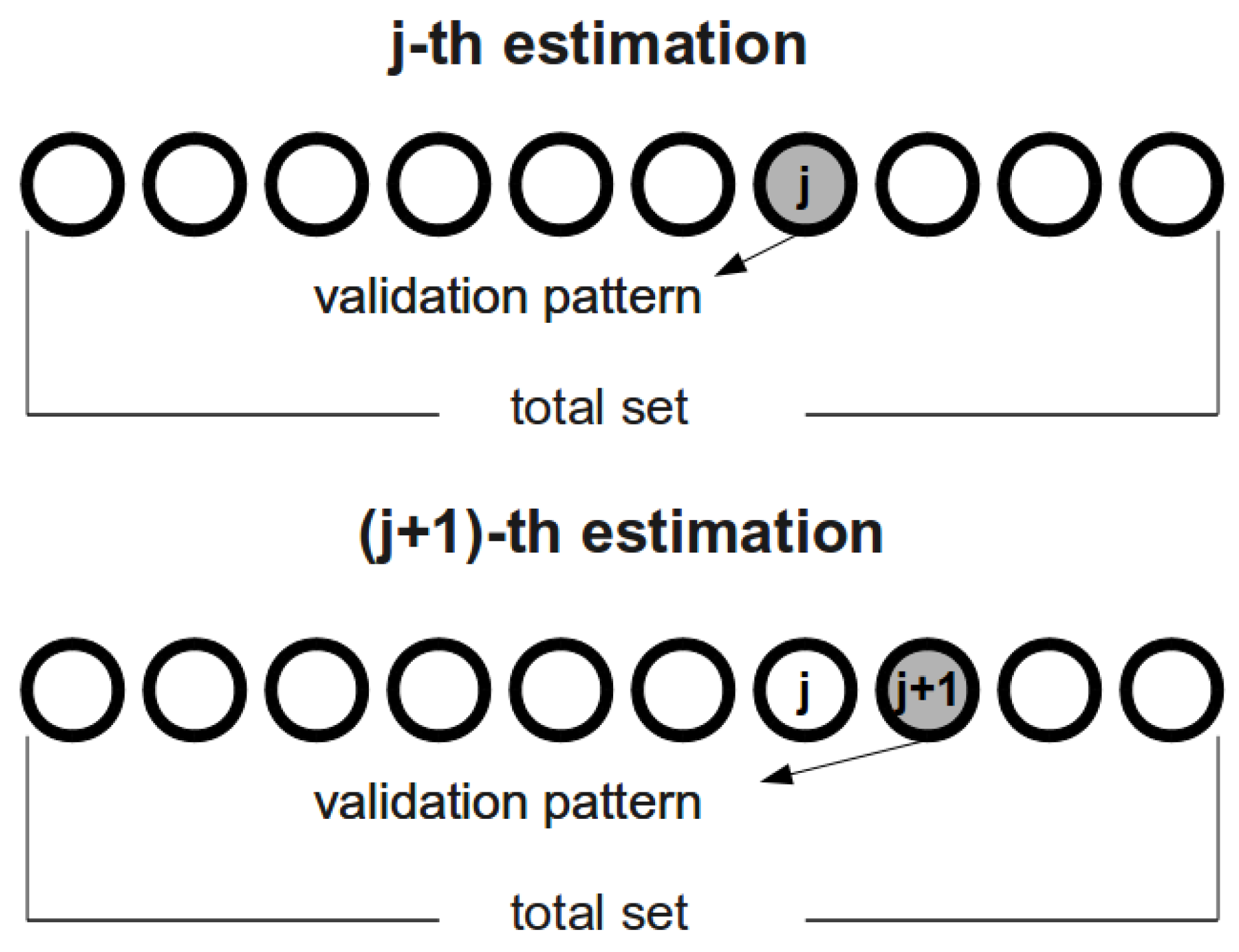
The cross-validation procedure used in this paper.
Figure 3.
The cross-validation procedure used in this paper.
In this framework, a specific facility of our tool, the so called “all-frame” or “leave-one-out” cross-validation procedure, is used. We try to estimate precipitation values (targets) from indices data (inputs) but, due to the quite short time series available, we maximize the extension of the training set: each precipitation value is estimated at a time after the exclusion of the correspondent inputs-target pattern from the training set used for fixing the connection weights. This procedure is simply sketched in
Figure 3, where our total set of patterns is divided in two subsets. The white circles represent the elements (patterns) of our training set, while the grey circle (one single element) represents the validation set. The relative composition of the training and validation sets change at each step of an iterative procedure of training + validation cycles. A “hole” in the complete set represents our validation set and moves across this total set of patterns, thus permitting the estimation of all precipitation values at the end of the procedure.
In this paper, we adopt the all-frame procedure just described, for both the neural model and the multi-linear control regression.
4. Nonlinear Attribution of Precipitation Changes
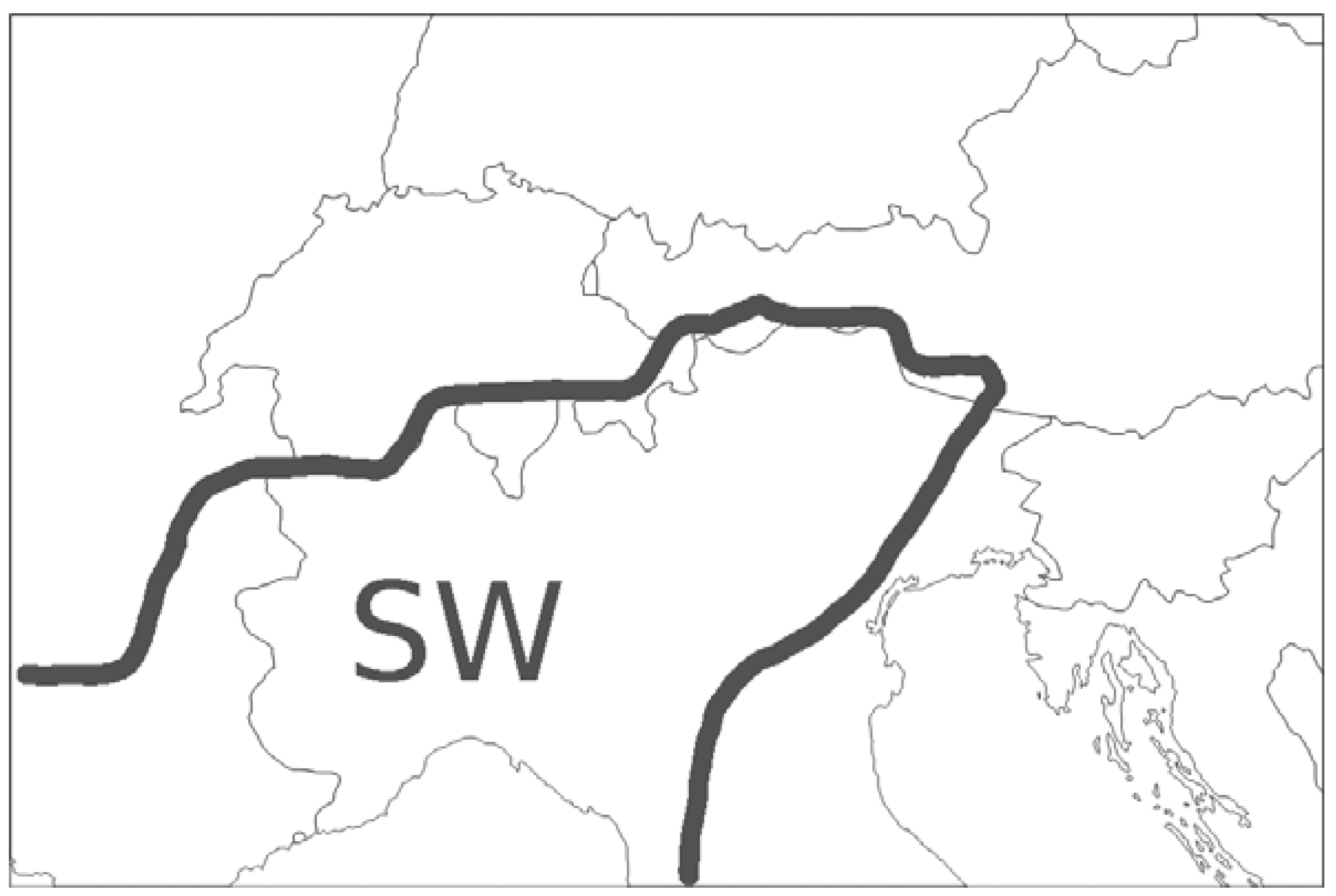
The main scopes of this paper are to “attribute” the behavior of time-changes of mean (annual and seasonal) precipitation inside the SW part of the GAR region, and to possibly find models that are able to reconstruct precipitation anomalies from data about indices of certain circulation patterns.
In every system, the easiest way to test the possible influence of certain variables (hypothetical causes) on another target is the calculation of the Pearson linear correlation coefficient R between each “cause” and the target itself, in a bivariate manner. But, as is well known, climate is a nonlinear system, so that even variables, which do not show high linear correlations with the target, can however be influential on the target by means of more complex and nonlinear relationships. Thus, as a first step of investigation, we perform a bivariate analysis between each index of circulation patterns and precipitation, not only through the standard R coefficient, but also by means of its nonlinear analogue Rnl, the so called correlation ratio.
The square of correlation ratio can be written as [
19]:
Using an NN jargon, we can consider the target (precipitation in our case) as the dependent variable and one input at a time (value of a circulation index) as the independent variable. Here Rnl is defined in terms of the average of the target for every specific i-th value of the chosen input: in fact, qi is the sample size for the i-th class of the input,
is the average target for the i-th class of the input,
is the average target on all the classes of the input and
is the total size of the set considered here. The whole range of input values is divided into several intervals that are labelled as classes.
Even if Rnl does not measure all types of nonlinearities, its calculation on our problem permits one to understand if some nonlinearities are hidden in the relationships among the variables considered here. Furthermore, as a consequence of this bivariate analysis, the inputs to be considered for an optimal nonlinear multiple regression (via NNs) could be different from the variables “suggested” by the calculation of the standard linear correlation coefficient R.
The results of this bivariate correlation analysis are summarized in
Table 1. Furthermore, due to a possible delayed influence of Pacific patterns (retarded correlations of ENSO phases with precipitation in the GAR were recently found [
10]), in
Table 2, cross-correlations are tested for the influence of ENSO on precipitation in the forthcoming seasons, up to a nine-month lag. For instance, the significant value that is found at the intersection of spring ENSO and summer precipitation means that ENSO could lead p by three months. In these Tables, extended winter is the four-month period December–March and the values in bold text indicate linear correlations and cross-correlations, which were found to be significant under a two-tail Student’s
t test with a 95% confidence interval.
Table 1.
Calculation of R and Rnl (indices vs. precipitation) for several periods.
Table 1.
Calculation of R and Rnl (indices vs. precipitation) for several periods.
| Period | Correlation index
vs. p | NAO | EA | AO | SCAN | EAWR | ABI | EBI | ENSO |
|---|
| Spring | R | −0.001 | 0.009 | −0.011 | 0.376 | −0.184 | −0.175 | 0.252 | 0.266 |
| Rnl | −0.245 | 0.535 | −0.229 | 0.570 | −0.595 | −0.400 | 0.439 | 0.485 |
| Summer | R | −0.001 | −0.232 | −0.220 | 0.418 | −0.048 | 0.010 | 0.562 | −0.357 |
| Rnl | −0.458 | −0.433 | −0.363 | 0.505 | −0.360 | 0.488 | 0.628 | −0.529 |
| Autumn | R | −0.136 | 0.106 | −0.281 | 0.589 | 0.003 | −0.172 | 0.334 | −0.251 |
| Rnl | −0.363 | 0.454 | −0.292 | 0.702 | 0.564 | −0.405 | 0.451 | −0.554 |
| Winter | R | −0.222 | −0.076 | −0.142 | 0.170 | 0.056 | 0.129 | 0.173 | −0.133 |
| Rnl | −0.586 | −0.420 | −0.237 | 0.469 | 0.223 | 0.418 | 0.580 | −0.375 |
| Extended winter | R | −0.397 | −0.297 | −0.465 | 0.521 | −0.223 | 0.312 | 0.098 | 0.152 |
| Rnl | −0.607 | −0.540 | −0.548 | 0.670 | −0.367 | 0.538 | 0.424 | 0.391 |
| Year | R | −0.055 | −0.031 | −0.276 | 0.471 | −0.080 | 0.031 | 0.350 | −0.196 |
| Rnl | −0.255 | −0.464 | −0.363 | 0.612 | −0.464 | 0.502 | 0.462 | −0.407 |
Table 2.
Linear and nonlinear cross-correlations (ENSO vs. precipitation).
Table 2.
Linear and nonlinear cross-correlations (ENSO vs. precipitation).
| ENSO | Cross−correlation | Spring | Summer | Autumn | Winter |
|---|
| Precipitation | | | | | |
|---|
| Spring | R | 0.266 | −0.101 | 0.079 | 0.073 |
| Rnl | 0.485 | −0.530 | 0.620 | 0.435 |
| Summer | R | −0.297 | −0.357 | 0.073 | 0.180 |
| Rnl | −0.560 | −0.529 | 0.346 | 0.292 |
| Autumn | R | −0.169 | −0.284 | −0.251 | −0.210 |
| Rnl | −0.557 | −0.545 | −0.554 | −0.412 |
| Winter | R | −0.011 | −0.143 | −0.064 | −0.133 |
| Rnl | −0.672 | −0.452 | −0.270 | −0.375 |
An accurate analysis of these Tables allows us to appreciate some relevant connections between circulation patterns and precipitation in the SW part of the Greater Alpine Region. These results may be summarized in the following points.
Extended winter appears to be the most sensitive season as far as the influence of these circulation patterns on precipitation is concerned: almost all indices are significantly correlated with this variable.
On the other hand, for the same reason, the influence of SCAN seems to be important in almost all periods.
The well known influence of NAO on precipitation in extended winter is recognized, but influences of the same magnitude are also due to AO and SCAN.
Among the blocking indices, EBI appears to be quite important in summer and autumn.
ENSO presents a relevant correlation in summer, but also some important anti-cross-correlations.
Sometimes, indices that show low linear correlations are endowed with a higher correlation value in terms of Rnl. This suggests the existence of nonlinear relationships between these indices and precipitation and may induce us to consider even these indices in the following attempt at finding models which are able to reconstruct precipitation behavior once fed by the data of these circulation patterns.
After this preliminary bivariate analysis, our next step of investigation is to search for NN models that, by considering data about indices as inputs, are able to reconstruct precipitation changes in the various periods.
In doing so, due to the limited length of patterns, we cannot build networks that include all the indices as inputs, because in this case, we should fall into overfitting conditions. Thus, just combinations of 3 indices are considered as inputs and our networks are characterized by a maximum of 4 neurons inserted in a single hidden layer. The choice of these combinations of inputs follows two criteria: all the indices that are linearly significant in
Table 1 and
Table 2 are considered; even indices which are not linearly significant but show high nonlinear correlations are taken into account.
After many runs of networks endowed with distinct inputs and adopting the cross-validation procedure described in
Section 3, quite interesting results are obtained: the NN performances on the validation set are summarized in
Table 3 by calculating the linear correlations (values of
R) between targets and outputs. The performance of leave-one-out multi-linear regressions is also shown for comparison.
Table 3.
NN performance of the best models and comparison with multi-linear regression.
Table 3.
NN performance of the best models and comparison with multi-linear regression.
| Period | Inputs(indices) | NN performance | Multi-linear performance |
|---|
| Spring | SCAN, EAWR, ENSO (autumn) | 0.275 | 0.181 |
| Summer | ENSO, SCAN, EBI | 0.618 | 0.567 |
| Autumn | SCAN, ENSO, EAWR | 0.531 | 0.530 |
| Winter | NAO, EA, ENSO (spring) | 0.302 | 0.070 |
| Extended winter | AO, SCAN, ABI | 0.537 | 0.469 |
| Year | EA, SCAN, ENSO | 0.470 | 0.438 |
Some specific considerations may be derived from results presented in
Table 3. In particular:
The importance of SCAN (previously recognized in the bivariate analysis) is confirmed by the need of including this index as an input almost everywhere in order to obtain the best NN models.
The relevance of ENSO on precipitation in the SW part of the GAR region appears to be quite high, either as direct or time-lagged influence.
The role of NAO seems quite retrenched and, in order to obtain the best NN performance, we needed to insert this input just for winter. AO and other indices appear to be more relevant in extended winter.
As far as this last point is concerned, it is worthwhile to note that attempts at inserting AO and NAO as inputs in the same networks lead to bad performance, even when these indices are highly correlated with the targets. This fact is quite understandable because these two indices are strongly correlated with each other while, as is well known (see, for instance, [
20]), NNs require input variables as independent as possible for an optimal performance.
In all periods, except autumn, we are able to find an NN model that leads to a reconstruction of precipitation anomalies that is better than that of the multi-linear one. This result has been recovered even by calculation of other indices of performance (MAE, MSE), here not shown.
In any case, however, this reconstruction performance is not very high: elsewhere [
21] we find better results for the reconstruction of temperature anomalies in the same sector of GAR. This confirms that catching the behavior of precipitation is a very difficult task.
As a final remark, we note that sometimes, the values of
R in
Table 3 are lower than the analogous ones for single variables in
Table 1 and
Table 2. This should not be a surprise, because in the multivariate runs we adopt the leave-one-out method and this usually leads to a quite high decrease in performance when applied to short records of data, as in our case.
An example of the reconstruction performance of our NN models is presented in
Figure 4 for the precipitation anomalies in the summer season.
Figure 4.
NN reconstruction (blue line) of the percentage precipitation anomalies in summer (red line) with respect to the mean of the period 1901–2000.
Figure 4.
NN reconstruction (blue line) of the percentage precipitation anomalies in summer (red line) with respect to the mean of the period 1901–2000.
This Figure shows that inter-annual variability of precipitation is caught quite well by our NN model: many peaks and oscillations in the graph are “recognized” by the model itself, even if, surely, the accuracy of reconstruction is not completely satisfying and the unexplained variance in the data remains quite high. Furthermore, in this and other cases, the NN models lead to a quite low bias, while the multi-linear reconstructions usually show a larger value of bias. In
Figure 4, the reconstruction bias could seem quite high, because the average NN forecast (113%) is above the 100% line, but we must consider that also the observed precipitation anomalies of this period are positively biased (105%) with respect to the mean values of the whole last century, so that the NN effective bias is not so high.
In short, by NN models, we are able to catch the qualitative behavior of precipitation climate variability in the region considered in this investigation, but the quantitative reconstruction of the real values of precipitation anomalies is still quite rough. This is probably due to a mixing of factors: for instance, the difficulty of the problem itself, but also the shortness of our time series does not allow us to use more input variables and a more complex structure in our networks without falling into overfitting problems.
In the past, investigations about European climate variability concentrated on the role of NAO and ENSO (see [
10] for an updated research of this kind), while more recently, a study on the influence of other circulation patterns has been performed, but through linear methods and the study referred to quite a limited region [
22]. If one compares our outcomes with the results presented in [
10,
22], he finds that the role of NAO could be somewhat retrenched, while ENSO cross-correlations may be still considered as quite influential. Furthermore, even if obtained by different methods and the study referred to a more extended region, our outcomes corroborate the results presented in [
22] about the importance of SCAN and some blocking indices on the precipitation behavior.
Finally, the additional importance of the present study should be found in the fully nonlinear method adopted here and in the attempt at working out a model for reconstructing precipitation changes in our case-study region. This treatment has shown interesting results, which should be obviously refined in the future.
5. Conclusions and Prospects
In this paper, a nonlinear analysis of the influence of eight circulation patterns on precipitation changes in an extended Italian Alpine region has been performed. To the best of our knowledge, it represents the first extensive study of this kind with nonlinear methods.
The results obtained here permit one to weight the role of these indices on precipitation in the different seasons: influences of SCAN and ENSO (even at delayed times) are always very important, while AO and NAO are contributing factors just in winter and extended winter. By explicitly working out NN models, which try to reconstruct precipitation changes and climate variability at this SW-GAR scale, additional information can be obtained. In particular, the influence of these circulation patterns may be re-evaluated when they are nonlinearly “mixed” as inputs of an NN. Furthermore, this method allows us to obtain NN models that are able to catch the climate variability of precipitation at a regional scale, even if they have to be improved in order to obtain more precise estimations of precipitation amounts.
Thus, the first prospect of further development is surely the adoption of a more complex NN model. But, as specified above, this implies the availability of a longer time series of indices.
Furthermore, this kind of studies opens concrete prospects of performing reliable downscaling activities. In fact, if future GCMs shall show improved ability to simulate the behavior of circulation patterns and we are able to find a transfer function from these patterns to precipitation anomalies in the past, a major road could be opened for obtaining reliable future scenarios of precipitation changes at regional scale.


