Linking Spatial Patterns of Groundwater Table Dynamics and Streamflow Generation Processes in a Small Developed Catchment


Abstract
:1. Introduction
- Does streamflow respond equally to rainfall input throughout the whole stream reach and which runoff sources are contributing to stormflow?
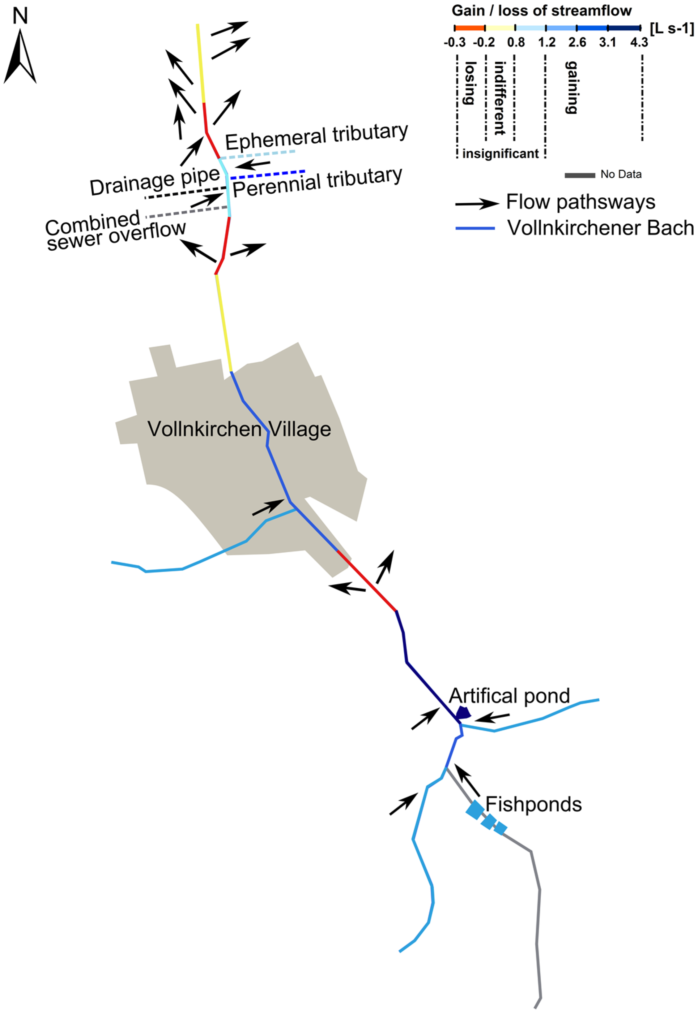
- Is the studied stream a gaining or losing system?
- Do groundwater head levels and flow dynamics respond to variations in stream stage and is this flow behavior changing throughout the year?
2. Materials and Methods
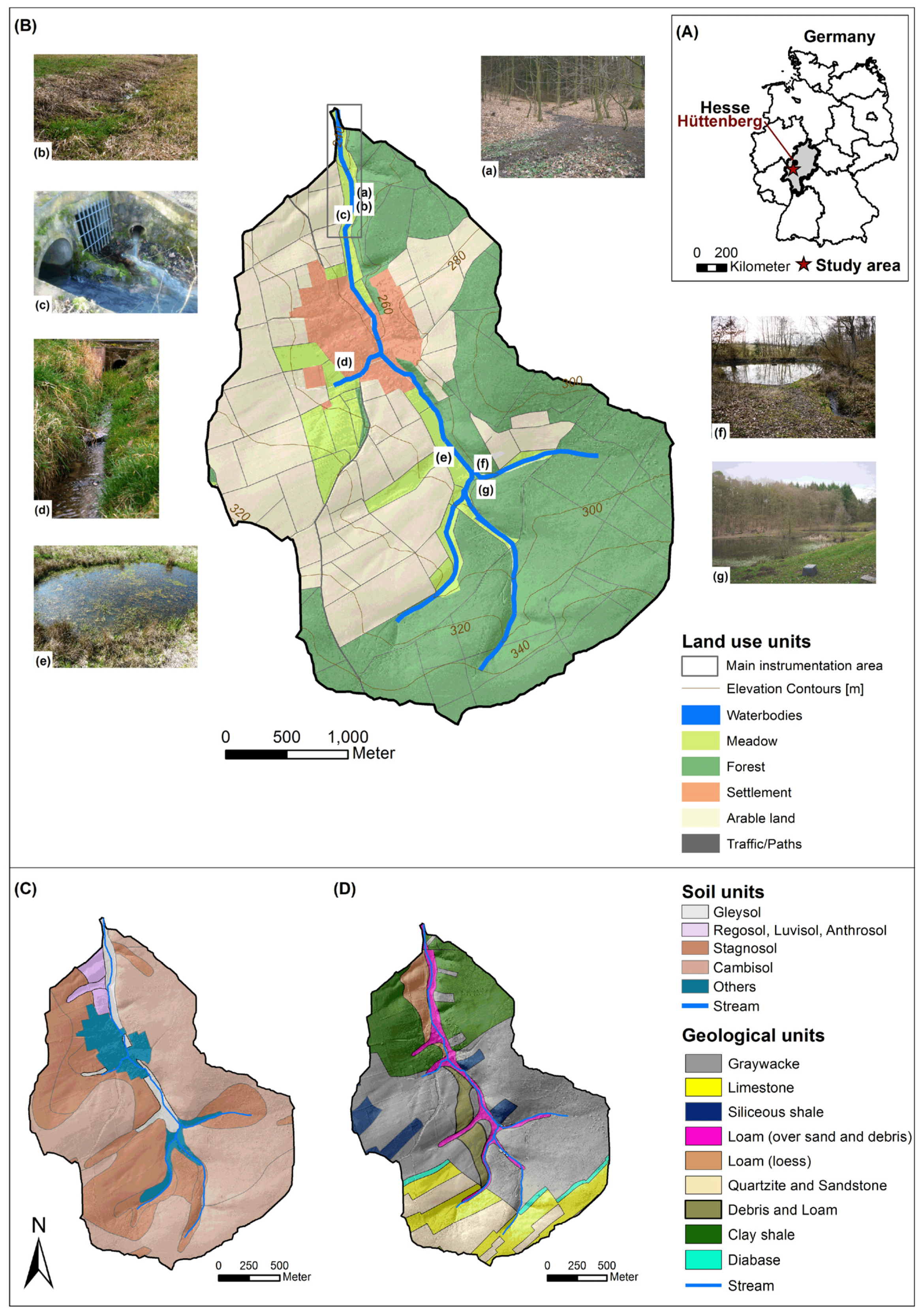
2.1. Study Area
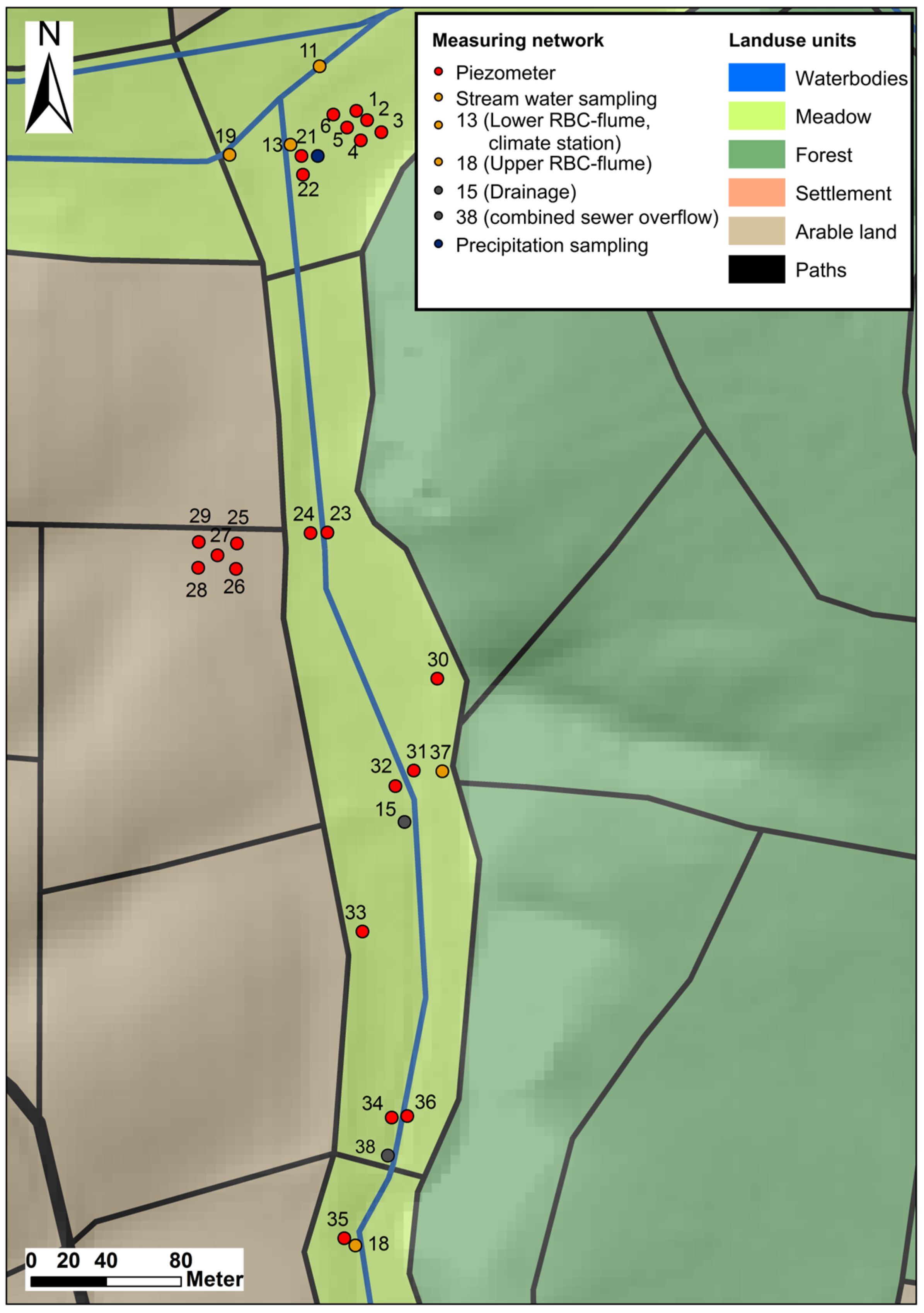
2.2. Monitoring Network


| Piezometer | Location | Land Use | Groundwater Level Measurements | Height a.s.l. (m) | Minimum Distance to Stream (m) |
|---|---|---|---|---|---|
| 1 | Outlet Vollnkirchener Bach | Meadow | Automatic+manual | 234.2 | 38.3 |
| 2 | 234.2 | 43.4 | |||
| 3 | 234.2 | 50.4 | |||
| 4 | 234.4 | 39.1 | |||
| 5 | 234.2 | 32.4 | |||
| 6 | 234.3 | 25.8 | |||
| 21 | 234.9 | 6.7 | |||
| 22 | 235.1 | 6.5 | |||
| 23 | Eastern stream-site | 238.9 | 0.8 | ||
| 24 | Towards 23, western stream-site | 238.6 | 5.2 | ||
| 25 | Western hillslope site | Arable land | 239.6 | 44.8 | |
| 26 | 240.2 | 46.2 | |||
| 27 | 240.4 | 55.8 | |||
| 28 | 241.2 | 66.3 | |||
| 29 | 240.3 | 65.0 | |||
| 30 | Eastern stream-site, close to forest | Meadow | Manual | 240.5 | 34.8 |
| 31 | Beside point source, eastern stream-site | Automatic+manual | 240.9 | 4.3 | |
| 32 | Towards 31, western stream-site | 241.0 | 5.0 | ||
| 33 | Western stream-site | Manual | 243.9 | 30.2 | |
| 34 | Western stream-site | Automatic+manual | 245.1 | 4.0 | |
| 35 | Beside upper RBC-flume, western stream-site | 247.1 | 6.9 | ||
| 36 | Eastern stream-site | 245.0 | 1.0 |
2.3. Hydrodynamic Methods and Data Analysis
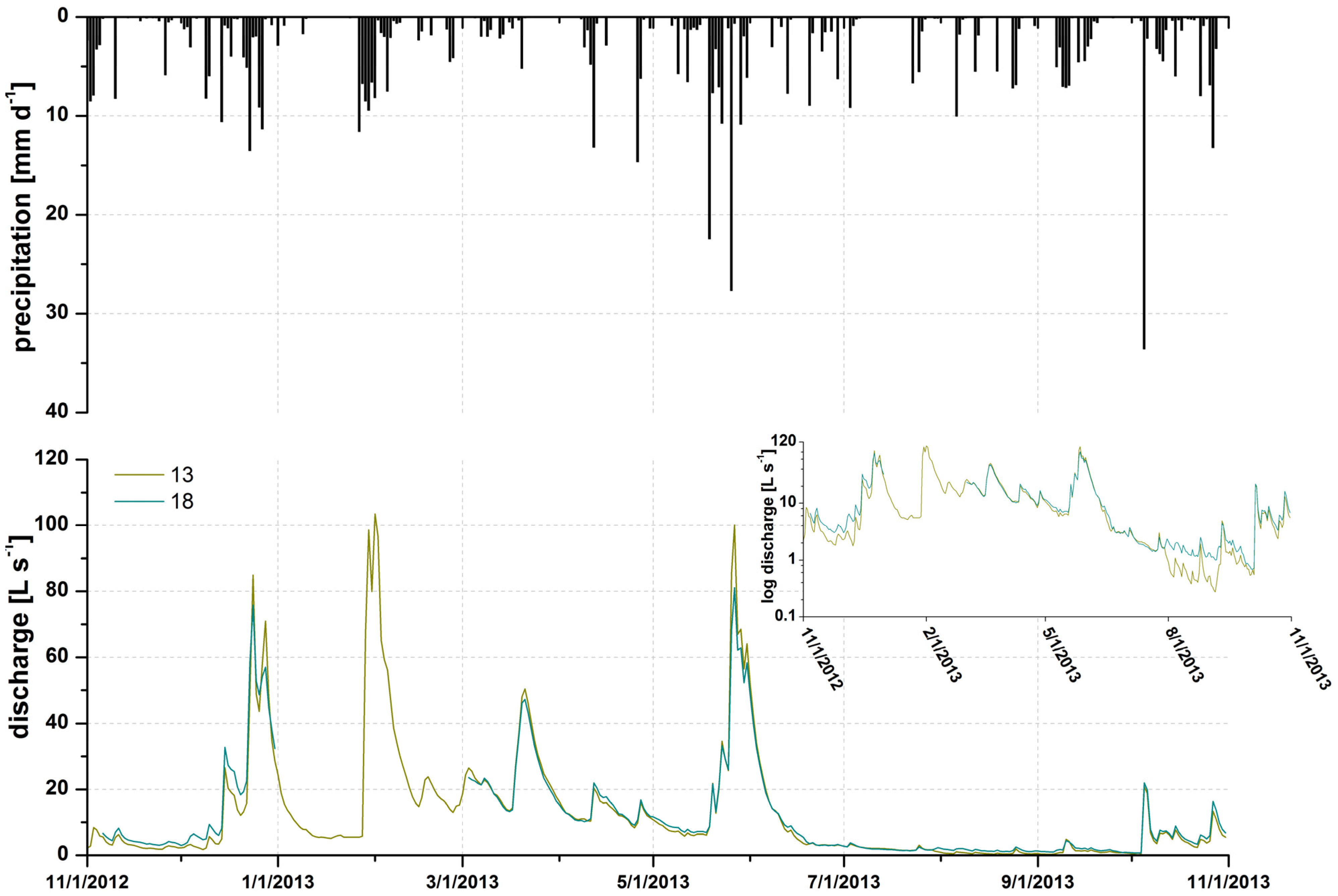
2.3.1. Streamflow Dynamics
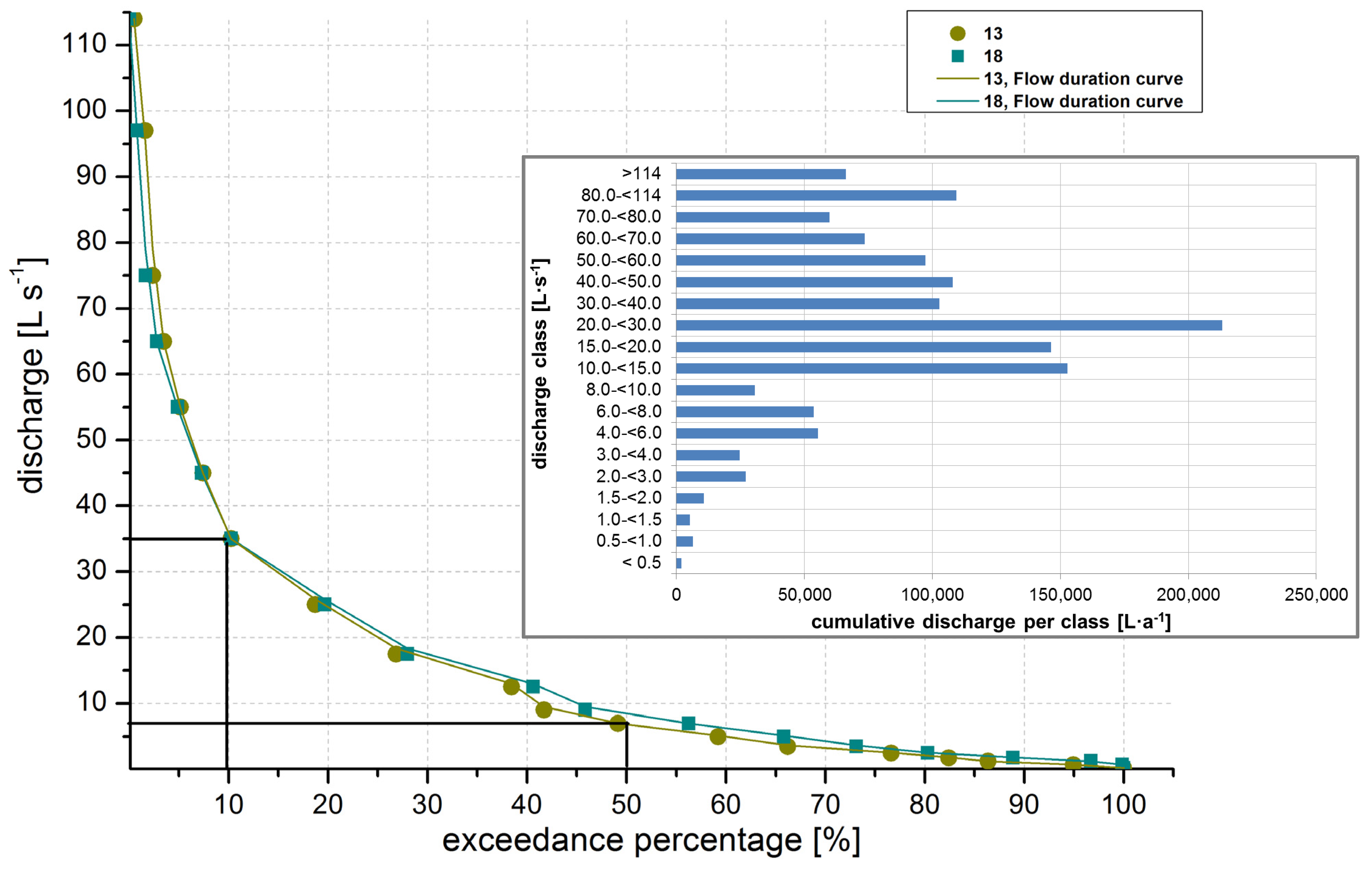
Flow Duration Curve Analysis
| Method | Aim | Location/Sites |
|---|---|---|
| Flow duration curve | Characterize the frequency of occurrence of a certain discharge | 13, 18 |
| Lag-to-peak time | Define catchment response time to rainfall events | 13, 18, combined sewer overflow |
| Hydrograph separation | Determine contribution of event/pre-event water to stormflow event | 13 |
| Incremental stream gauging | Detect gaining/losing reaches along the Vollnkirchener Bach | 12 sampling points along the creek |
| Groundwater flow direction | Define groundwater flux dynamics under different saturation conditions | All piezometers |
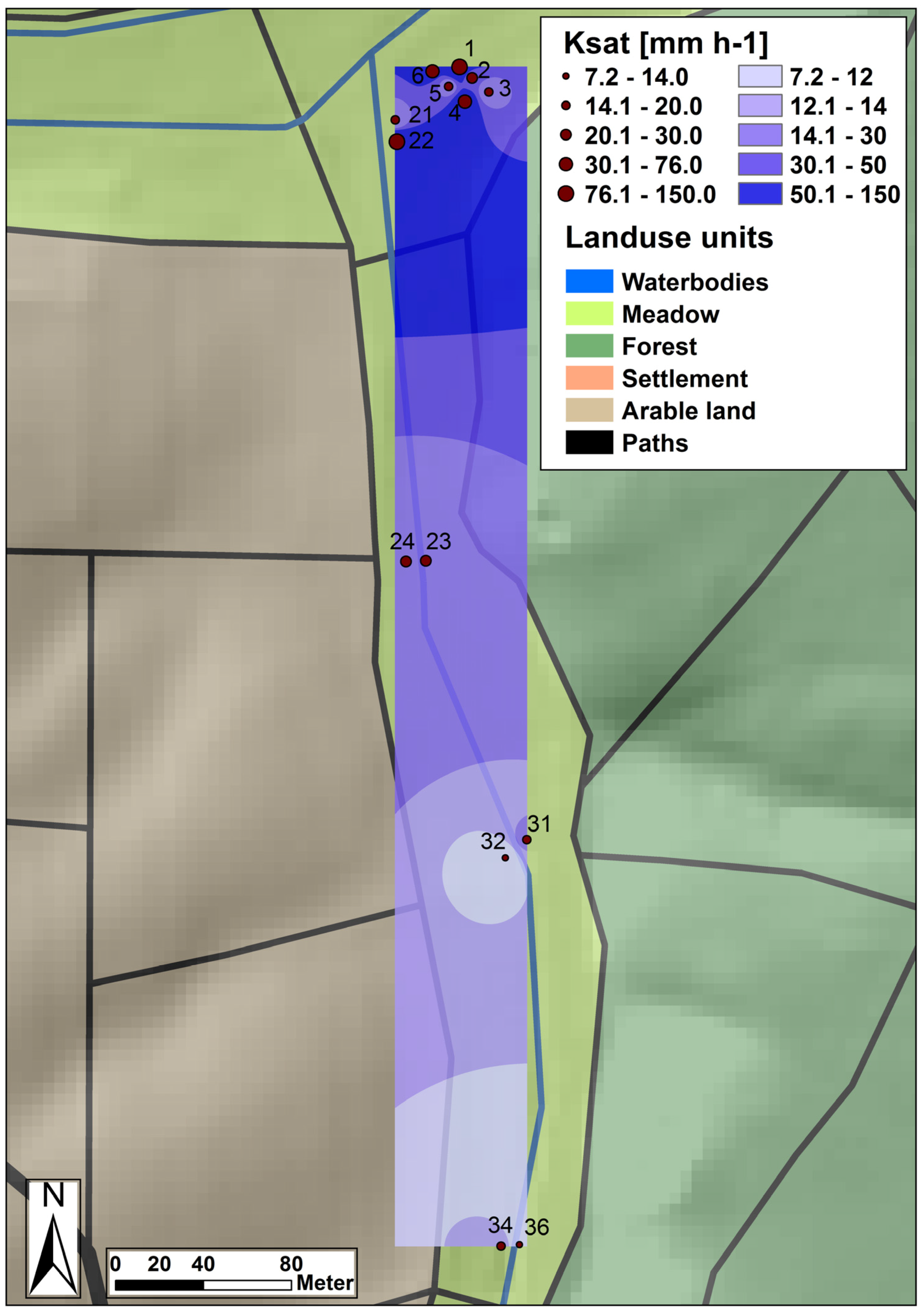
| Slug tests | Estimate saturated hydraulic conductivity of aquifer material | Piezometers: 1–6, 21–24, 31, 32, 34, 36 |
| Correlation of groundwater head level response | Identify groundwater relationships and patterns | All automatically measured piezometers |
| Correlation of groundwater head levels vs. discharge | Characterize groundwater response to discharge | All automatically measured piezometers vs. 13, 18 |
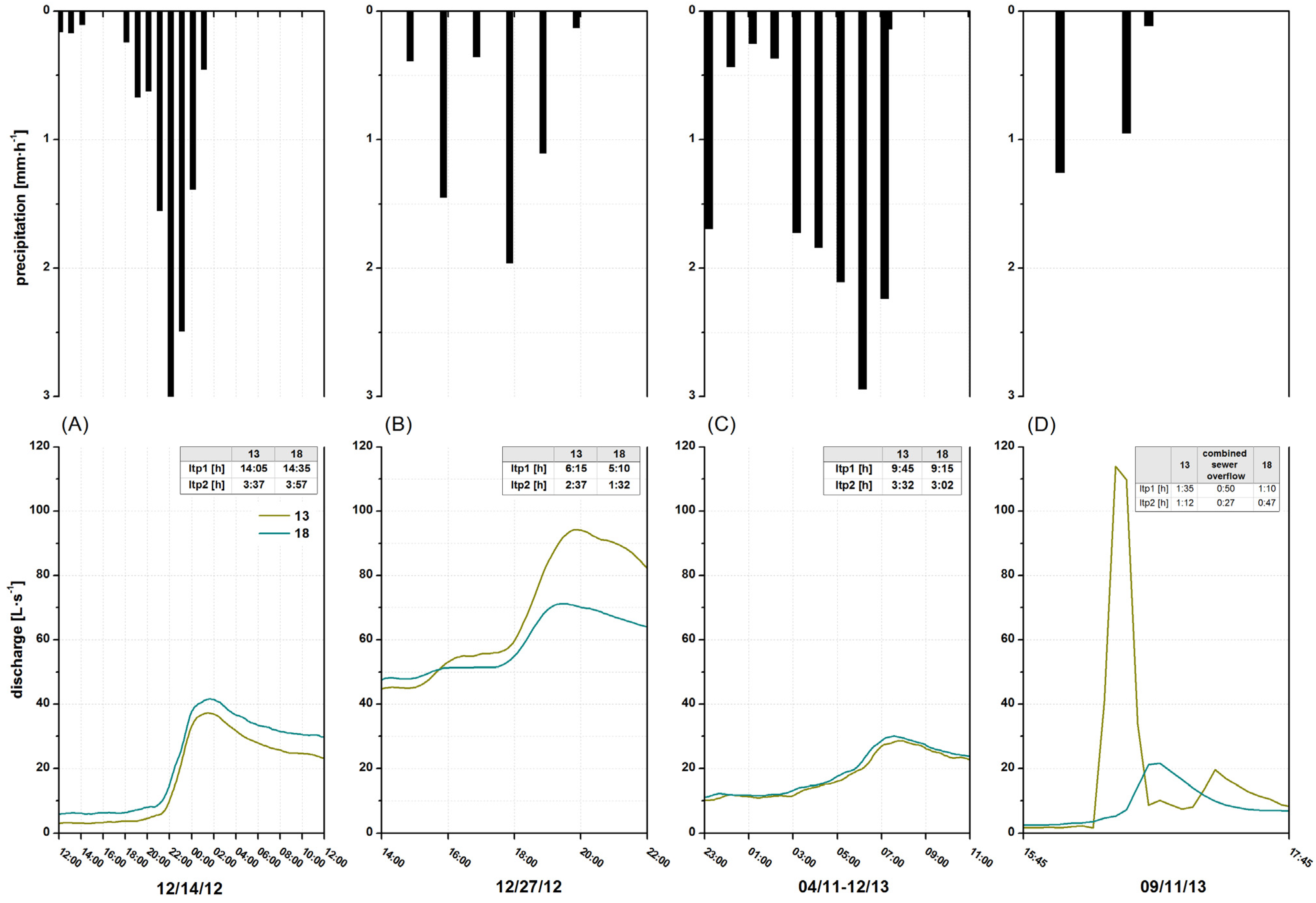
Lag-to-Peak Times and Rainfall-Runoff Behavior
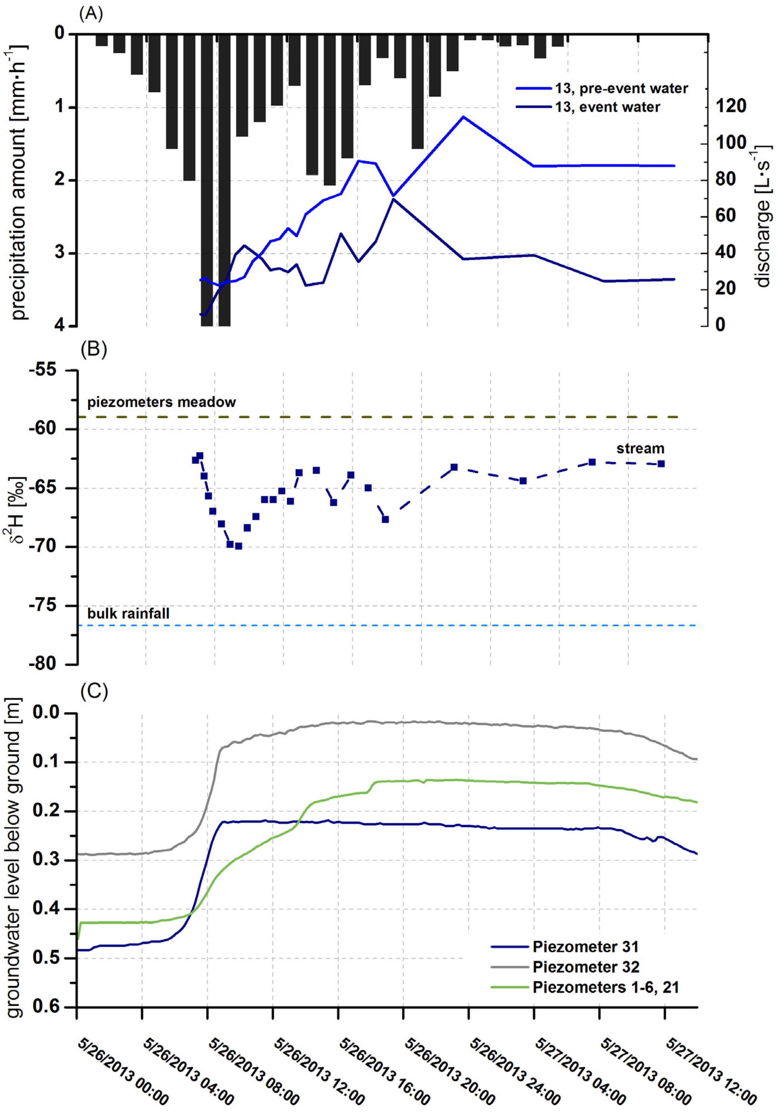
Hydrograph Separation
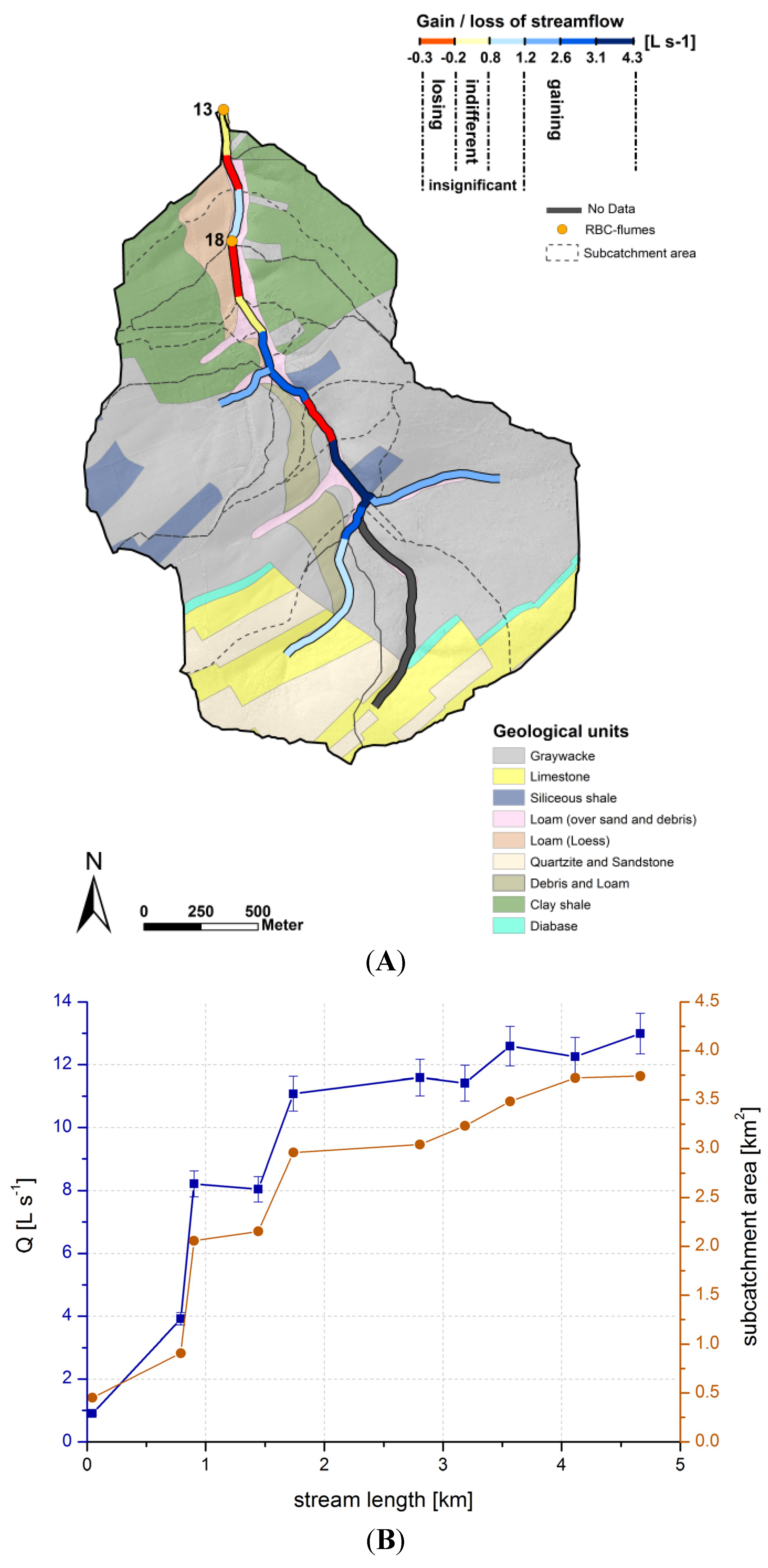
Incremental Stream Gauging
2.3.2. Groundwater Dynamics
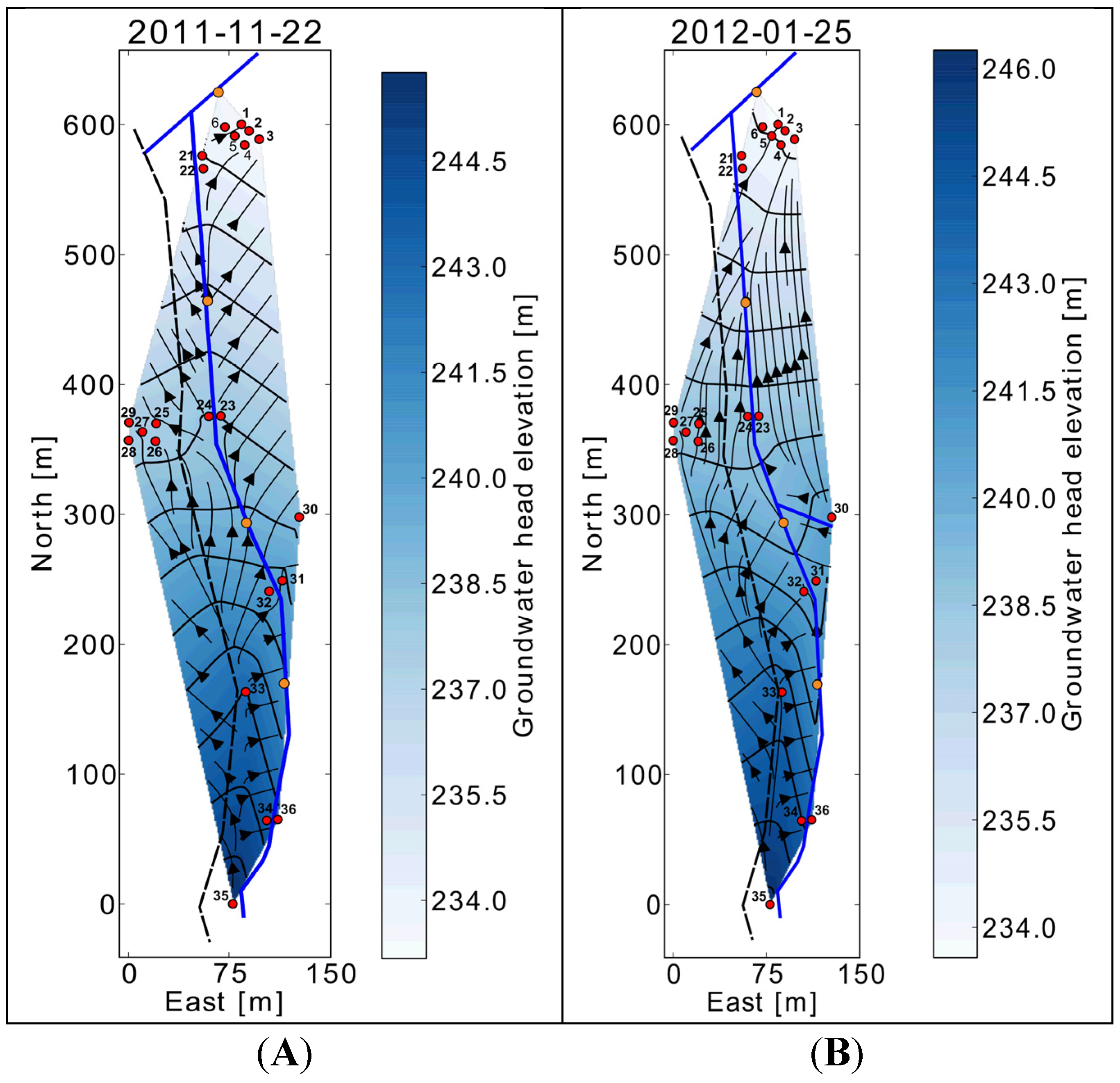
Groundwater Flow Direction Analyses
Aquifer Hydraulic Conductivity
Groundwater Head Level Correlations and Piezometric Stream Stage Response
3. Results
3.1. Streamflow Dynamics
3.1.1. Flow Duration Curve Analyses
3.1.2. Lag- to-Peak Times and Rainfall-Runoff Behavior


| Rainfall | AP (mm) | Discharge (L·s−1) | ltp1 (h) | ltp2 (h) | |||||||||||||||
|---|---|---|---|---|---|---|---|---|---|---|---|---|---|---|---|---|---|---|---|
| Q0 | Qmax | Qmax/Q0 | |||||||||||||||||
| Duration (h) | Total (mm) | Mean (mm·h−1) | 3d | 5d | 14d | 13 | 18 | 13 | 18 | combined sewer overflow | 13 | 18 | 13 | 18 | combined sewer overflow | 13 | 18 | combined sewer overflow | |
| Event-type I (N = 3) | |||||||||||||||||||
| Min | 5:15 | 4.9 | 0.7 | 0.0 | 9.5 | 19.3 | 3.3 | 5.2 | 18.4 | 20.5 | 4.2 | 3.4 | 7:25 | 7:25 | 3:27 | 3:57 | |||
| Max | 13:40 | 11.3 | 1.7 | 3.9 | 14.0 | 49.0 | 4.4 | 6.2 | 38.6 | 42.0 | 11.6 | 8.0 | 14:05 | 14:35 | 7:37 | 7:12 | |||
| Event-type II (N = 12) | |||||||||||||||||||
| Min | 1:30 | 1.5 | 0.8 | 1.5 | 2.0 | 11.5 | 12.7 | 11.9 | 62.2 | 59.0 | 1.2 | 1.1 | 2:40 | 2:20 | 7:20 | 2:17 | 1:32 | 5:42 | |
| Max | 25:30 | 28.2 | 2.2 | 27.7 | 42.9 | 95.6 | 83.9 | 73.4 | 140.5 | 110.1 | 10.0 | 7.2 | 25:30 | 25:40 | 12:37 | 12:47 | |||
| Event-type III (N = 4) | |||||||||||||||||||
| Min | 7:45 | 9.3 | 1.1 | 0.0 | 0.0 | 0.6 | 0.6 | 0.8 | 18.1 | 18.7 | 2.3 | 2.1 | 8:30 | 8:40 | 3:32 | 3:02 | |||
| Max | 26:15 | 35.6 | 1.5 | 31.0 | 31.2 | 49.4 | 11.5 | 12.4 | 45.7 | 46.5 | 74.3 | 55.4 | 18:20 | 18:20 | 10:52 | 9:27 | |||
| Event-type IV (N = 6) | |||||||||||||||||||
| Min | 1:05 | 2.3 | 0.8 | 0.0 | 0.0 | 6.8 | 0.1 | 0.8 | 5.1 | 7.2 | 34.5 | 4.8 | 3.6 | 1:00 | 0:40 | 0:30 | 0:42 | 0:12 | 0:27 |
| Max | 9:20 | 29.1 | 3.7 | 16.9 | 22.3 | 23.2 | 4.5 | 5.9 | 21.8 | 21.6 | >114.0 | 53.8 | 15.9 | 3:30 | 3:00 | 2:50 | 1:30 | 0:55 | 0:35 |
3.1.3. Hydrograph Separation
3.1.4. Incremental Stream Gauging


3.2. Groundwater Dynamics
3.2.1. Groundwater Flow Directions


3.2.2. Aquifer Hydraulic Conductivity

3.2.3. Groundwater Head Level Correlations and Piezometric Stream Stage Response
| Location | Site | 13 | 18 | 1 | 2 | 3 | 4 | 5 | 6 | 21 | 22 | 23 | 24 | 25 | 26 | 27 | 28 | 29 | 31 | 32 | 34 | 35 | 36 |
|---|---|---|---|---|---|---|---|---|---|---|---|---|---|---|---|---|---|---|---|---|---|---|---|
| Lower RBC-flume | 13 | x | |||||||||||||||||||||
| Upper RBC-flume | 18 | 0.96 | x | ||||||||||||||||||||
| Meadow (outlet) | 1 | 0.79 | 0.75 | x | |||||||||||||||||||
| 2 | 0.75 | 0.70 | 0.95 | x | |||||||||||||||||||
| 3 | 0.85 | 0.82 | 0.88 | 0.88 | x | ||||||||||||||||||
| 4 | 0.83 | 0.78 | 0.78 | 0.80 | 0.89 | x | |||||||||||||||||
| 5 | 0.89 | 0.85 | 0.94 | 0.92 | 0.93 | 0.89 | x | ||||||||||||||||
| 6 | 0.76 | 0.81 | 0.85 | 0.82 | 0.84 | 0.70 | 0.96 | x | |||||||||||||||
| 21 | 0.81 | 0.85 | 0.81 | 0.78 | 0.84 | 0.72 | 0.94 | 0.89 | x | ||||||||||||||
| 22 | 0.73 | 0.68 | 0.89 | 0.89 | 0.87 | 0.49 | 0.90 | 0.94 | 0.90 | x | |||||||||||||
| Eastern stream-site | 23 | 0.90 | 0.88 | 0.85 | 0.82 | 0.86 | 0.87 | 0.92 | 0.77 | 0.80 | 0.80 | x | |||||||||||
| Western stream-site | 24 | 0.92 | 0.88 | 0.87 | 0.83 | 0.86 | 0.85 | 0.91 | 0.77 | 0.79 | 0.84 | 0.96 | x | ||||||||||
| Arable land, western stream-site | 25 | 0.51 | 0.46 | 0.43 | 0.43 | 0.54 | 0.81 | 0.54 | 0.36 | 0.25 | 0.01 | 0.52 | 0.57 | x | |||||||||
| 26 | 0.58 | 0.46 | 0.49 | 0.48 | 0.63 | 0.84 | 0.51 | 0.34 | 0.39 | 0.00 | 0.60 | 0.62 | 1.00 | x | |||||||||
| 27 | 0.70 | 0.51 | 0.50 | 0.50 | 0.74 | 0.78 | 0.15 | 0.43 | 0.55 | 0.00 | 0.68 | 0.68 | 0.91 | 0.99 | x | ||||||||
| 28 | 0.59 | 0.48 | 0.51 | 0.50 | 0.64 | 0.85 | 0.52 | 0.36 | 0.39 | 0.00 | 0.61 | 0.63 | 1.00 | 1.00 | 1.00 | x | |||||||
| 29 | 0.29 | 0.50 | 0.20 | 0.44 | 0.32 | 0.60 | 0.00 | 0.04 | 0.40 | 0.10 | 0.52 | 0.61 | 0.82 | 0.98 | 0.86 | 0.98 | x | ||||||
| Eastern stream-site | 31 | 0.22 | 0.20 | 0.30 | 0.28 | 0.26 | 0.17 | 0.35 | 0.23 | 0.47 | 0.67 | 0.18 | 0.18 | 0.02 | 0.05 | 0.01 | 0.07 | 0.22 | x | ||||
| Towards 31, western stream-site | 32 | 0.69 | 0.67 | 0.57 | 0.47 | 0.56 | 0.47 | 0.78 | 0.54 | 0.66 | 0.63 | 0.59 | 0.63 | 0.15 | 0.22 | 0.48 | 0.24 | 0.20 | 0.40 | x | |||
| Western stream-site | 34 | 0.92 | 0.87 | 0.88 | 0.82 | 0.85 | 0.90 | 0.94 | 0.74 | 0.78 | 0.81 | 0.93 | 0.95 | 0.61 | 0.59 | 0.58 | 0.61 | 0.35 | 0.20 | 0.67 | x | ||
| Beside 18, western stream-site | 35 | 0.66 | 0.51 | 0.69 | 0.69 | 0.68 | 0.93 | 0.87 | 0.55 | 0.64 | 0.33 | 0.61 | 0.67 | 0.94 | 0.81 | 0.82 | 0.80 | 0.00 | 0.97 | 0.60 | 0.66 | x | |
| Towards 34, eastern stream-site | 36 | 0.86 | 0.82 | 0.91 | 0.87 | 0.92 | 0.81 | 0.93 | 0.73 | 0.63 | 0.92 | 0.86 | 0.89 | 0.59 | 0.58 | 0.19 | 0.61 | 0.00 | 0.09 | 0.46 | 0.91 | 0.94 | x |

4. Discussion
5. Conclusions: Conceptualizing Groundwater-Surface Water Interactions from the Reach-Scale to the Catchment-Scale

Acknowledgments
Author Contributions
Conflicts of Interest
References
- Klapper, H. Historical Change of Large Alluvial Rivers: Western Europe; Petts, G.E., Möller, H., Roux, A.L., Eds.; John Wiley and Sons Ltd.: Chichester, UK, 1990; Volume 75, p. 355. [Google Scholar]
- Allan, J.D. Landscapes and riverscapes: The influence of land use on stream ecosystems. Annu. Rev. Ecol. Evol. Syst. 2004, 35, 257–284. [Google Scholar]
- Cox, M.H.; Su, G.W.; Constantz, J. Heat, chloride, and specific conductance as ground water tracers near streams. Ground Water 2007, 45, 187–195. [Google Scholar]
- Unland, N.P.; Cartwright, I.; Andersen, M.S.; Rau, G.C.; Reed, J.; Gilfedder, B.S.; Atkinson, A.P.; Hofmann, H. Investigating the spatio-temporal variability in groundwater and surface water interactions: A multi-technique approach. Hydrol. Earth Syst. Sci. 2013, 17, 3437–3453. [Google Scholar]
- Baxter, C.; Hauer, F.R.; Woessner, W.W. Measuring groundwater–stream water exchange: New techniques for installing minipiezometers and estimating hydraulic conductivity. Trans. Am. Fish. Soc. 2003, 132, 493–502. [Google Scholar]
- Brown, V.A.; McDonnell, J.J.; Burns, D.A.; Kendall, C. The role of event water, a rapid shallow flow component, and catchment size in summer stormflow. J. Hydrol. 1999, 217, 171–190. [Google Scholar]
- Crespo, P.; Buecker, A.; Feyen, J.; Vache, K.B.; Frede, H.-G.; Breuer, L. Preliminary evaluation of the runoff processes in a remote montane cloud forest basin using Mixing Model Analysis and Mean Transit Time. Hydrol. Process. 2012, 26, 3896–3910. [Google Scholar]
- Didszun, J.; Uhlenbrook, S. Scaling of dominant runoff generation processes: Nested catchments approach using multiple tracers. Water Resour. Res. 2008, 44. [Google Scholar] [CrossRef]
- Munyaneza, O.; Wenninger, J.; Uhlenbrook, S. Identification of runoff generation processes using hydrometric and tracer methods in a meso-scale catchment in Rwanda. Hydrol. Earth Syst. Sci. 2012, 16, 1991–2004. [Google Scholar]
- Hrachowitz, M.; Bohte, R.; Mul, M.L.; Bogaard, T.A.; Savenije, H.H.G.; Uhlenbrook, S. On the value of combined event runoff and tracer analysis to improve understanding of catchment functioning in a data-scarce semi-arid area. Hydrol. Earth Syst. Sci. 2011, 15, 2007–2024. [Google Scholar]
- Kalbus, E.; Reinstorf, F.; Schirmer, M. Measuring methods for groundwater—Surface water interactions: a review. Hydrol. Earth Syst. Sci. 2006, 10, 873–887. [Google Scholar]
- Kendall, C.; McDonnell, J.J. Isotope Tracers in Catchment Hydrology, 1st ed.; Elsevier: Amsterdam, The Netherlands, 1998. [Google Scholar]
- Wels, C.; Cornett, R.J.; Lazerte, B.D. Hydrograph separation: A comparison of geochemical and isotopic tracers. J. Hydrol. 1991, 122, 253–274. [Google Scholar]
- Wenninger, J.; Uhlenbrook, S.; Lorentz, S.; Leibundgut, C. Identification of runoff generation processes using combined hydrometric, tracer and geophysical methods in a headwater catchment in South Africa. Hydrol. Sci. J. 2008, 53, 65–80. [Google Scholar]
- Lana-Renault, N.; Latron, J.; Regüés, D. Streamflow response and water-table dynamics in a sub-Mediterranean research catchment (Central Pyrenees). J. Hydrol. 2007, 347, 497–507. [Google Scholar]
- Studienlandschaft Schwingbachtal. Available online: http://www.uni-giessen.de/cms/fbz/fb09/institute/ilr/studienlandschaft/startseite (accessed on 17 February 2014).
- Engineering Geology and the Environment; Marinos, P.G.; Koukis, G.C.; Tsiambaos, G.C.; Stournaras, G.C. (Eds.) CRC Press: Boca Raton, FL, USA, 1997.
- Mazor, E. Chemical and Isotopic Groundwater Hydrology, 3rd ed.; CRC Press: Boca Raton, FL, USA, 2003. [Google Scholar]
- Lauer, F.; Frede, H.-G.; Breuer, L. Uncertainty assessment of quantifying spatially concentrated groundwater discharge to small streams by distributed temperature sensing. Water Resour. Res. 2013, 49, 400–407. [Google Scholar]
- DWD Deutscher Wetterdienst—Wetter und Klima, Bundesministerium für Verkehr und digitale Infrastruktur. Available online: http://dwd.de (accessed on 17 February 2014).
- Fankhauser, R. Measurement properties of tipping bucket rain gauges and their influence on brain runoff simulation. Water Sci. Technol. 1997, 36, 7–12. [Google Scholar]
- Maksimović, Č.; Bužek, L.; Petrović, J. Corrections of rainfall data obtained by tipping bucket rain gauge. Atmos. Res. 1991, 27, 45–53. [Google Scholar]
- Xia, Y. Optimization and uncertainty estimates of WMO regression models for the systematic bias adjustment of NLDAS precipitation in the United States. J. Geophys. Res. Atmos. 2006, 111. [Google Scholar] [CrossRef]
- HLUG Hessisches Landesamt für Umwelt und Geologie. Available online: http://www.hlug.de (accessed on 16 January 2014).
- HVBG Hessische Verwaltung für Bodenmanagement und Geoinformation. Available online: http://www.hvbg.hessen.de (accessed on 16 January 2014).
- Food and Agriculture Organization of the United Nations. World Reference Base for Soil Resources 2006: A Framework for International Classification, Correlation and Communication; World Soil Resources Reports 103; Food and Agriculture Organization: Rome, Italy, 2006. [Google Scholar]
- Eijkelkamp RBC flumes. Available online: http://en.eijkelkamp.com/products/water/hydrological-research/water-discharge-measurements/rbc-flumes.htm (accessed on 13 January 2014).
- Ali, H. Fundamentals of Irrigation and On-farm Water Management; Springer: New York, NY, USA, 2010; Volume 1. [Google Scholar]
- Database—Studienlandschaft Schwingbachtal. Available online: http://fb09-pasig.umwelt.uni-giessen.de:8081/ (accessed on 17 February 2014).
- Davie, T. Fundamentals of Hydrology; Taylor & Francis: Oxford, UK, 2008. [Google Scholar]
- Dingman, S.L. Physical Hydrology, 2nd ed.; Waveland Press Inc.: Long Grove, IL, USA, 2002. [Google Scholar]
- Rusjan, S.; Mikoš, M. Assessment of hydrological and seasonal controls over the nitrate flushing from a forested watershed using a data mining technique. Hydrol. Earth Syst. Sci. 2008, 12, 645–656. [Google Scholar]
- Cook, P.G.; Herczeg, A.L. Environmental Tracers in Subsurface Hydrology; Springer: New York, NY, USA, 2000. [Google Scholar]
- Bohté, R.; Mul, M.L.; Bogaard, T.A.; Savenije, H.H.G.; Uhlenbrook, S.; Kessler, T.C. Hydrograph separation and scale dependency of natural tracers in a semi-arid catchment. Hydrol. Earth Syst. Sci. Discuss. 2010, 7, 1343–1372. [Google Scholar]
- Buttle, J.M. Isotope hydrograph separations and rapid delivery of pre-event water from drainage basins. Prog. Phys. Geogr. 1994, 18, 16–41. [Google Scholar]
- Newman, B.; Tanweer, A.; Kurttas, T. IAEA Standard Operating Procedure for the Liquid-Water Stable Isotope Analyser 2009. Available online: http://www-naweb.iaea.org/napc/ih/documents/other/laser_procedure_rev12 (accessed on 5 February 2013).
- Craig, H. Standard for reporting concentrations of deuterium and oxygen-18 in natural waters. Science 1961, 133, 1833–1834. [Google Scholar]
- LGR Los Gatos Research. Greenhouse Gas, isotope and trace gas analyzers. Available online: http://www.lgrinc.com/ (accessed on 5 February 2013).
- Cey, E.E.; Rudolph, D.L.; Parkin, G.W.; Aravena, R. Quantifying groundwater discharge to a small perennial stream in southern Ontario, Canada. J. Hydrol. 1998, 210, 21–37. [Google Scholar]
- Harte, P.T.; Kiah, R.G. Measured river leakages using conventional streamflow techniques: the case of Souhegan River, New Hampshire, USA. Hydrogeol. J. 2009, 17, 409–424. [Google Scholar]
- Winter, T.C.; Harvey, J.W.; Franke, O.L.; Alley, W.M. Ground Water and Surface Water: A Single Resource; U.S. Geological Survey Circular 1139; DIANE Publishing: Collingdale, PA, USA, 1999. [Google Scholar]
- Day, T.J. On the precision of salt dilution gauging. J. Hydrol. 1976, 31, 293–306. [Google Scholar]
- Moore, R.D. Introduction to Salt Dilution Gauging for Streamflow Measurement. Available online: http://www.docstoc.com/docs/74117190/Introduction-to-Salt-Dilution-Gauging-for-Streamflow-Measurement (accessed on 13 September 2013).
- Hongve, D. A revised procedure for discharge measurement by means of the salt dilution method. Hydrol. Process. 1987, 1, 267–270. [Google Scholar]
- Kilpatrick, F.A.; Cobb, E.D. Measurements of discharge using tracers. In Techniques of Water-Resources Investigations; Book 3; U.S. Geological Survey: Reston, VA, USA, 1985; p. 52. [Google Scholar]
- Boissonnat, J.-D.; Cazals, F. Smooth surface reconstruction via natural neighbour interpolation of distance functions. Comput. Geom. 2002, 22, 185–203. [Google Scholar]
- Zemansky, G.M.; McElwee, C.D. High-resolution slug testing. Ground Water 2005, 43, 222–230. [Google Scholar]
- Butler, J.J., Jr. The Design, Performance, and Analysis of Slug Tests; CRC Press LLC: Boca Raton, FL, USA, 1997. [Google Scholar]
- Singhal, B.B.S.; Gupta, R.P. Applied Hydrogeology of Fractured Rocks, 2nd ed.; Springer: New York, NY, USA, 2010. [Google Scholar]
- Hvorslev, M.J. Time lag and soil permeability in ground-water observations. Bulletin 1951, 36, 50. [Google Scholar]
- Anderson, A.E.; Weiler, M.; Alila, Y.; Hudson, R.O. Piezometric response in zones of a watershed with lateral preferential flow as a first-order control on subsurface flow. Hydrol. Process. 2010, 24, 2237–2247. [Google Scholar]
- Vogel, R.M.; Fennessey, N.M. Flow duration curves ii: A review of applications in water resources planning. J. Am. Water Resour. Assoc. 1995, 31, 1029–1039. [Google Scholar]
- Hewlett, J.D.; Fortson, J.C.; Cunningham, G.B. The effect of rainfall intensity on storm flow and peak discharge from forest land. Water Resour. Res. 1977, 13, 259–266. [Google Scholar]
- Han, S.; Xu, D.; Wang, S. Runoff formation from plot, field, to small catchment with shallow groundwater table and dense drainage system in agricultural North Huaihe River Plain, China. Hydrol. Earth Syst. Sci. Discuss. 2012, 9, 4235–4262. [Google Scholar]
- Biron, P.M.; Roy, A.G.; Courschesne, F.; Hendershot, W.H.; Côté, B.; Fyles, J. The effects of antecedent moisture conditions on the relationship of hydrology to hydrochemistry in a small forested watershed. Hydrol. Process. 1999, 13, 1541–1555. [Google Scholar]
- Ali, G.A.; Roy, A.G.; Turmel, M.-C.; Courchesne, F. Multivariate analysis as a tool to infer hydrologic response types and controlling variables in a humid temperate catchment. Hydrol. Process. 2010, 24, 2912–2923. [Google Scholar]
- Hooper, R.P.; Shoemaker, C.A. A Comparison of chemical and isotopic hydrograph separation. Water Resour. Res. 1986, 22, 1444–1454. [Google Scholar]
- Caissie, D.; Pollock, T.L.; Cunjak, R.A. Variation in stream water chemistry and hydrograph separation in a small drainage basin. J. Hydrol. 1996, 178, 137–157. [Google Scholar]
- Mul, M.L.; Savenije, H.H.G.; Uhlenbrook, S. Spatial rainfall variability and runoff response during an extreme event in a semi-arid catchment in the South Pare Mountains, Tanzania. Hydrol. Earth Syst. Sci. 2009, 13, 1659–1670. [Google Scholar]
- Carey, S.K.; Quinton, W.L. Evaluating runoff generation during summer using hydrometric, stable isotope and hydrochemical methods in a discontinuous permafrost alpine catchment. Hydrol. Process. 2005, 19, 95–114. [Google Scholar]
- Klaus, J.; McDonnell, J.J. Hydrograph separation using stable isotopes: Review and evaluation. J. Hydrol. 2013, 505, 47–64. [Google Scholar]
- McDonnell, J.J.; Bonell, M.; Stewart, M.K.; Pearce, A.J. Deuterium variations in storm rainfall: Implications for stream hydrograph separation. Water Resour. Res. 1990, 26, 455–458. [Google Scholar]
- Pionke, H.B.; Gburek, W.J.; Folmar, G.J. Quantifying stormflow components in a Pennsylvania watershed when 18O input and storm conditions vary. J. Hydrol. 1993, 148, 169–187. [Google Scholar]
- Banks, E.W.; Simmons, C.T.; Love, A.J.; Cranswick, R.; Werner, A.D.; Bestland, E.A.; Wood, M.; Wilson, T. Fractured bedrock and saprolite hydrogeologic controls on groundwater/surface-water interaction: A conceptual model (Australia). Hydrogeol. J. 2009, 17, 1969–1989. [Google Scholar]
- Banks, E. Groundwater-Surface Water Interactions in the Cox, Lenswood and Kersbrook Creek Catchments, Western Mount Lofty Ranges, South Australia; Science, Monitoring and Information Division, Department for Water, Government of Australia: Adeleide, Australia, 2010.
- Mastrocicco, M.; Vignoli, G.; Colombani, N.; Zeid, N.A. Surface electrical resistivity tomography and hydrogeological characterization to constrain groundwater flow modeling in an agricultural field site near Ferrara (Italy). Environ. Earth Sci. 2010, 61, 311–322. [Google Scholar]
- Yang, Y.J.; Gates, T.M. Wellbore skin effect in slug-test data analysis for low-permeability geologic materials. Ground Water 1997, 35, 931–937. [Google Scholar]
- Rovey II, C.W.; Niemann, W. L. Wellskins and slug tests: where’s the bias? J. Hydrol. 2001, 243, 120–132. [Google Scholar]
- Landon, M.K.; Rus, D.L.; Harvey, F.E. Comparison of instream methods for measuring hydraulic conductivity in sandy streambeds. Ground Water 2001, 39, 870–885. [Google Scholar]
- Baxter, C.V.; Hauer, F.R. Geomorphology, hyporheic exchange, and selection of spawning habitat by bull trout (Salvelinus confluentus). Can. J. Fish. Aquat. Sci. 2000, 57, 1470–1481. [Google Scholar]
- Butler, J.J.; McElwee, C.D.; Liu, W. Improving the quality of parameter estimates obtained from slug tests. Ground Water 1996, 34, 480–490. [Google Scholar]
- Krause, S.; Bronstert, A.; Zehe, E. Groundwater–surface water interactions in a North German lowland floodplain—Implications for the river discharge dynamics and riparian water balance. J. Hydrol. 2007, 347, 404–417. [Google Scholar]
- McDonnell, J.J. Are all runoff processes the same? Hydrol. Process. 2013, 27, 4103–4111. [Google Scholar]
- Tromp-van Meerveld, H.J.; McDonnell, J.J. Threshold relations in subsurface stormflow: 2. The fill and spill hypothesis. Water Resour. Res. 2006, 42. [Google Scholar] [CrossRef]
- Gabrielli, C.P.; McDonnell, J.J.; Jarvis, W.T. The role of bedrock groundwater in rainfall–runoff response at hillslope and catchment scales. J. Hydrol. 2012, 450–451, 117–133. [Google Scholar]
- Woessner, W.W. Stream and fluvial plain ground water interactions: Rescaling hydrogeologic thought. Ground Water 2000, 38, 423–429. [Google Scholar]
- Harvey, J.W.; Bencala, K.E. The Effect of streambed topography on surface-subsurface water exchange in mountain catchments. Water Resour. Res. 1993, 29, 89–98. [Google Scholar]
© 2014 by the authors; licensee MDPI, Basel, Switzerland. This article is an open access article distributed under the terms and conditions of the Creative Commons Attribution license (http://creativecommons.org/licenses/by/4.0/).
Share and Cite
Orlowski, N.; Lauer, F.; Kraft, P.; Frede, H.-G.; Breuer, L. Linking Spatial Patterns of Groundwater Table Dynamics and Streamflow Generation Processes in a Small Developed Catchment. Water 2014, 6, 3085-3117. https://doi.org/10.3390/w6103085
Orlowski N, Lauer F, Kraft P, Frede H-G, Breuer L. Linking Spatial Patterns of Groundwater Table Dynamics and Streamflow Generation Processes in a Small Developed Catchment. Water. 2014; 6(10):3085-3117. https://doi.org/10.3390/w6103085
Chicago/Turabian StyleOrlowski, Natalie, Florian Lauer, Philipp Kraft, Hans-Georg Frede, and Lutz Breuer. 2014. "Linking Spatial Patterns of Groundwater Table Dynamics and Streamflow Generation Processes in a Small Developed Catchment" Water 6, no. 10: 3085-3117. https://doi.org/10.3390/w6103085
APA StyleOrlowski, N., Lauer, F., Kraft, P., Frede, H.-G., & Breuer, L. (2014). Linking Spatial Patterns of Groundwater Table Dynamics and Streamflow Generation Processes in a Small Developed Catchment. Water, 6(10), 3085-3117. https://doi.org/10.3390/w6103085