Temporal Variability of Monthly Daily Extreme Water Levels in the St. Lawrence River at the Sorel Station from 1912 to 2010

Abstract

Although climate models predict that the impacts of climate change on the temporal variability of water levels in the St. Lawrence River will be seasonally-dependent, such a seasonal effect on the current variability of extreme water levels has never been analyzed. To address this, we analyzed the temporal variability of three hydrological variables (monthly daily maximums and minimums, as well as their ratio) of water levels in the St. Lawrence River measured at the Sorel station since 1912, as they relate to climate indices. As for stationarity, the shifts in the mean values of maximum and minimum water levels revealed by the Lombard method took place prior to 1970 for spring water levels, but after that year, for winter water levels. Changes in the winter stationarity are thought to mainly relate to the decreasing snowfall observed in the St. Lawrence River watershed after 1970. In contrast, for spring, these changes are likely primarily related to human activity (digging of the St. Lawrence Seaway and construction of dams). Two shifts in the mean values of fall minimum extreme water levels were highlighted. The first of these shifts, which occurred in the first half of the 1960s decade, can also be linked to human activity (digging of the St. Lawrence Seaway and construction of dams), whereas the second shift, observed after the 1970s for the months of November and December, can be linked to decreasing amounts of snow in winter. AMO (Atlantic Multidecadal Oscillation) is the climate index that is most frequently correlated negatively with the hydrologic variables, mainly in winter and spring.

1. Introduction

The St. Lawrence River is one of the World’s large rivers, known for its economic and ecological importance [1]. From an economic standpoint, it is one of the primary waterways for trade between North America and other continents, linking a significant portion of interior North America, the region surrounding the Great Lakes, with the rest of the World. Ecologically, the St. Lawrence River comprises fluviolacustrine and marine ecosystems rich in biodiversity, of which Lake Saint-Pierre (a widening of the river), part of the United Nations Educational, Scientific and Cultural Organization (UNESCO) World Network of Biosphere Reserves since 2000, is a striking example.

Because of its situation in a continental cool temperate climate and a highly industrialized and urbanized region, the St. Lawrence River is vulnerable to natural and/or anthropogenic environmental change. Among such changes, climate warming is the most likely to alter, to a varying extent, the natural hydrologic regime of the river with negative consequences on its biodiversity. Thus, according to hydroclimate models, climate warming will significantly alter the seasonal hydrologic cycle of the St. Lawrence and its tributaries [2]. These models predict an increase in streamflow or water levels in winter, due to increased precipitation as rain resulting from winter warming, on the one hand, and a significant decrease in streamflow in springtime resulting from decreasing snowfall in winter and increasing evapotranspiration caused by increasing temperature in springtime, on the other hand. From an ecological standpoint, these hydrological changes will lead, among other things, to a significant decrease in obligate wetland species abundance in favor of invasive terrestrial species, in particular [3].

Hydroclimate model predictions are partly supported by data based on the temporal variability of streamflow in the northeastern United States, where some of the St. Lawrence River tributaries are sourced. Thus, [4] noted a significant increase in winter streamflow in this region, but a decrease in springtime flows from 1912 to 2002. Such hydrological changes, the earlier occurrence of snowmelt in the spring, in particular, are also observed in other regions of North America, (e.g., [5,6,7,8]). From a climate standpoint, temperature in that part of the St. Lawrence River watershed located in southern Quebec shows a significant increase from 1960 to 2005 [9], while precipitation as snow decreased since 1980 [10] and precipitation as low-intensity rainfalls increased [11].

These various studies raise the following question: what are the impacts of the hydroclimatic changes observed in the St. Lawrence River watershed in Quebec on the temporal variability of its monthly daily extreme water levels? No study looking at the temporal variability of water levels or streamflow in the St. Lawrence River has addressed this question specifically (e.g., [12,13,14,15,16]). Moreover, these studies have not identified any impact of such hydroclimatic changes on the variability of water levels or streamflow in the St. Lawrence River. The main goal of this study is therefore to fill this gap. In addition, it also aims to test whether these monthly daily extreme water levels in the St. Lawrence are correlated with climate indices in winter and spring, the two seasons deemed most likely to show the effects of climate changes [2,3].

2. Methods

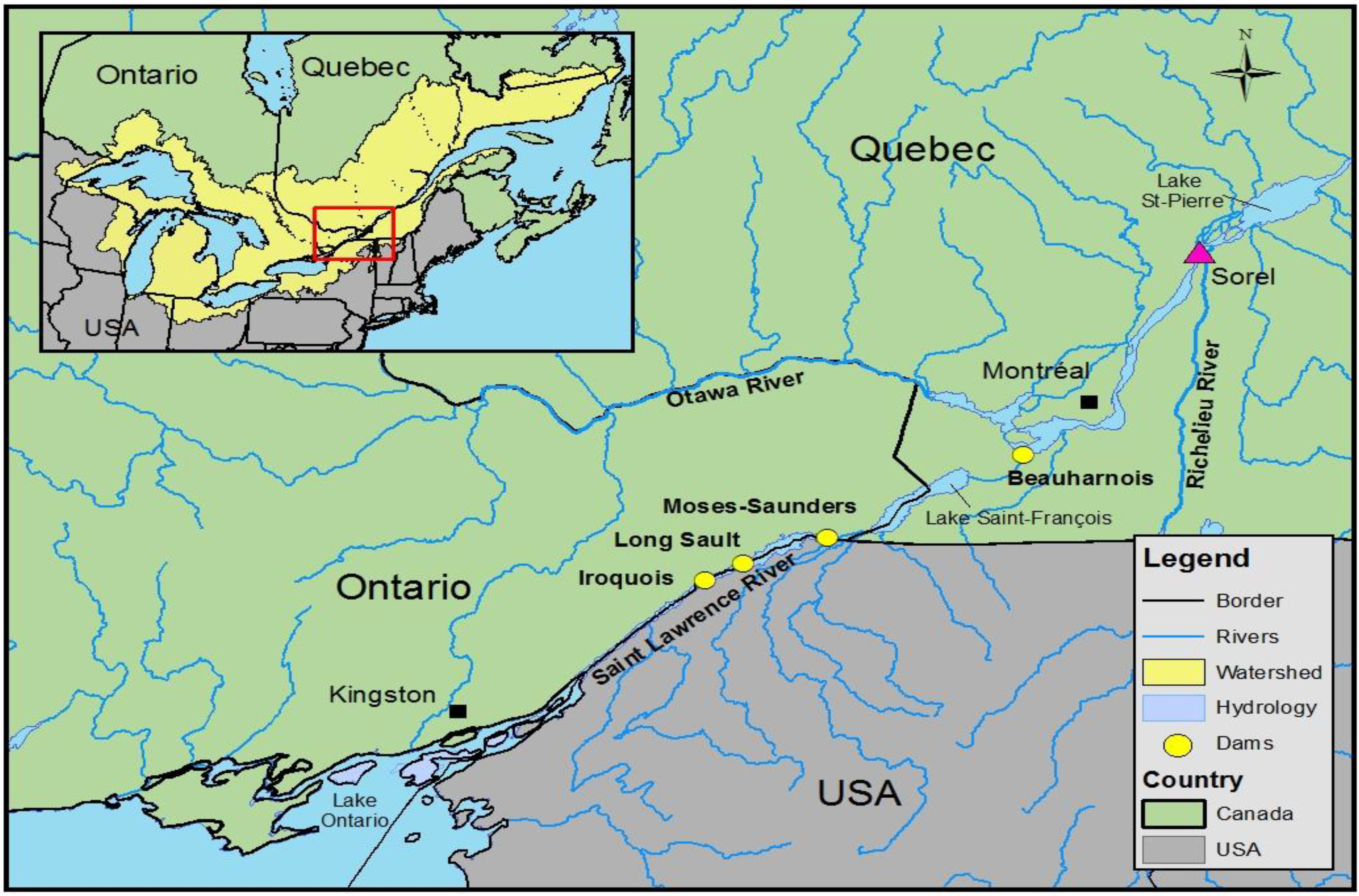
2.1. Study Area

The St. Lawrence River, Lake Ontario’s main natural outflow, is 3060 km-long, with a watershed covering 1,300,000 km². Nearly half of this area is located within the Province of Quebec, Canada (Figure 1), where its largest tributaries enter into it, including the two main ones: the Ottawa (179,000 km²) and Richelieu (22,000 km²) Rivers, respectively, located on the north and south shores of the St. Lawrence. The St. Lawrence River is fed by numerous tributaries draining varied climate regions. South shore tributaries drain a maritime-type temperate region, while north shore tributaries drain continental- and subarctic-type climate regions. To facilitate trade between North America’s Great Lakes Region and other continents, an extensive canal system was built along the St. Lawrence River channel and the Great Lakes starting in 1954. Known as the Great Lakes/St. Lawrence Seaway System, it is a 3700 km-long waterway linking the Atlantic Ocean with the Great Lakes and comprising a total of 19 locks and several dams used to regulate water levels in Lake Ontario and the St. Lawrence River. The dams are all located along the river between the cities of Cornwall and Montreal, the main ones being the Moses-Saunders, Long Sault, Iroquois and Beauharnois dams (Figure 1), of which the Moses-Saunders, built in 1960, is the largest [16]. In addition, the main tributary of the St. Lawrence, the Ottawa River, is also heavily regulated, comprising many reservoirs in which large amounts of water can be stored in springtime. As a result, a significant decrease in streamflow is observed in springtime downstream from these dams, while a significant increase in streamflow is observed in winter, causing a complete inversion of the natural annual cycle of streamflow (e.g., [17,18,19]). The effects of this inversion can be felt down to the confluence of the tributaries with the St. Lawrence. In the case of the Saint-Maurice River (43,000 km²), one of the main north shore tributaries, water input into the St. Lawrence decreases by 60% in springtime and increases by 20% in winter due to the presence of the reservoirs [20].

Water level data for the St. Lawrence River were taken from the Environment Canada website [21]. These data have been collected at the Sorel station, downstream from the confluence of the St. Lawrence River with its main tributary, the Ottawa River, since 1912 (Figure 1). Three hydrologic series were produced for each month: daily maximum extreme water levels (highest level measured during a given month of a given year); daily minimum extreme water levels (lowest level measured during a given month of a given year); and coefficients of immoderation (the ratio of the daily maximum and minimum extreme water levels). This coefficient of immoderation (CI) reflects the maximum amplitude of extreme water level variations during one month. These variations play a key role for aquatic fauna and flora [3,13,16]. The 12 months of the year are subdivided into four seasons: winter (January to March); spring (April to June); summer (July to September); and fall (October to December). The rationale for using water level analysis is two-fold: (1) the lack of flow data over a similarly long period at the Sorel station; and (2) the ability to then compare the temporal variability of water levels in the St. Lawrence River with that of water levels in Lake Ontario, the main outlet of which is the St. Lawrence. Finally, it should be mentioned that water level measurements take into account the effects of ice.

Figure 1. St-Lawrence watershed and location of the Sorel station.

Figure 1. St-Lawrence watershed and location of the Sorel station.

2.2. Statistical Analysis of Extreme Monthly Daily Water Levels

To identify a potential shift in the mean, we used the Lombard method [22,23], which constrains the type (abrupt or smooth) and timing (years) of changes affecting the mean and variance values of analyzed hydrological series. Suppose there is a series of observations, noted X₁,…X_n, where X_i is the observation taken at time T = i. These observations are supposed to be independent. One question of interest is to see whether the mean of this series has changed. If μ_i refers to the theoretical mean of X_i, then a possible pattern for the mean is given by Lombard’s smooth-change model, where:

(1)

In other words, the mean changes gradually from θ₁ to θ₂ between times T₁ and T₂. As a special case, one has the usual abrupt-change model when T₂ = T₁ + 1.

In order to test formally whether the mean in a series is stable or rather follows Model (5), one can use the statistical procedure introduced by [22]. To this end, define R_i as the rank of X_i among X₁,…X_n. Introduce the Wilcoxon score function ϕ (u) = 2u − 1 and define the rank score of X_i by:

(2)

where:

(3)

Lombard’s test statistic is:

(4)

where:

(5)

At the 5% levels of confidence, one concludes that the mean of the series changes significantly according to a pattern of Type (1) whenever S_n > 0.0403. This value corresponds to the theoretical (critical) values (see [22]) defining the significance thresholds (at 5%) for the test. Note that the equation proposed by [22] to detect multiple abrupt changes in the mean of a statistical series was also applied. This formula confirmed results obtained using Equation (5). It is important to note that the Lombard method was applied after autocorrelation was removed. This was done using the method proposed by [24].

The long-term trend of the temporal variability of extreme water levels was not derived as part of this study for the following reasons:

• From a statistical standpoint, there is a debate over the methods used to detect this long-term trend (e.g., [25]);
• From a hydrological standpoint, the long-term trend contribution to the determination of factors that cause shifts in the mean of a hydrological series is very limited;
• When data measured at a single station are analyzed, the effects of site and/or measuring device changes cannot be constrained using the long-term trend. Such changes can cause shifts in the mean values of the analyzed series;
• An analysis of the long-term trend does not bring out all the shifts in the mean that may affect a hydroclimatic series. Furthermore, the presence of multiple opposing shifts in the mean (decrease and increase) can mask this long-term trend.

As the last step, the three hydrologic series were correlated with monthly climate indices. Correlation was calculated on standardized data. Five climate indices were selected based on their demonstrated influence on the temporal variability of hydroclimatic variables in North America. These indices are AMO (Atlantic Multi-decadal Oscillation), AO (Arctic Oscillation), NAO (North Atlantic Oscillation), PDO (Pacific Decadal Oscillation) and SOI (Southern Oscillation Index). Climate indexes for AMO and PDO were taken from the following website: [26,27,28]. For each month, the three hydrologic variables (maximum, minimum and their ratio) were correlated with climate indices for the previous [r(−1)] and current [r(0)] month. The significance of coefficient of correlation values was checked using Monte Carlo re-sampling.

3. Results

3.1. Temporal Variability of Hydrological Variables

Results obtained using the Lombard method are presented in Table 1. For example, the temporal variability of extreme water levels in February (winter), May (Spring), August (summer) and November (fall) is shown respectively in Figure 2. For maximum water levels, shifts in the mean are observed in winter and spring. This shift took place after the 1970s decade for winter, but before that decade for spring. For minimum water levels, shifts in the mean took place in winter, spring and fall. The shifts in the mean occurred after the 1970s for winter, but prior to this decade for spring and fall, except for the month of June, for which the shifts in the mean took place after the 1970s. It is important to note that the timing of the shifts is not synchronous for different months of the same season, except for the months of February and March for maximum water levels and the months of April and May for minimum water levels. Comparison of mean values before and after the date of the shift reveals that maximum and minimum water levels decreased significantly over time (Table 2). The largest decrease is seen for the month of March for maximum water levels and the month of February for minimum water levels. In contrast, fall minimum water levels increased significantly over time, although this increase is generally smaller that the decrease observed for winter and spring. Finally, shifts in the mean had very little effects on the coefficients of immoderation series. These shifts are observed for the months of December to February. The means of CI values increased significantly in January and February, while they decreased in December (Table 2).

Table 1. Values of Lombard’s test statistic (S_n).

Month	Maxima		Minima		Coefficient of immoderation
	Sn	T1/T2	Sn	T1/T2	Sn	T1/T2
Winter
January	0.0453	1981/82	0.1704	1978/79	0.0717	1948/49
February	0.0461	1998/99	0.0920	1997/98	0.0411	1949/50
March	0.0969	1998/99	0.1698	1952/2004	0.0017	-
Spring
April	0.1156	1955/56	0.1698	1955/56	0.0029	-
May	0.0460	1947/48	0.1206	1956/57	0.0029	-
June	0.0526	1930/31	0.0473	1997/99	0.0150	-
Summer
July	0.0039	-	0.0015	-	0.0042	-
August	0.0289	-	0.0146	-	0.0311	-
September	0.0325	-	0.0272	-	0.0341	-
Fall
October	0.0476	1966/67	0.0491	1935/36	0.0104	-
November	0.0217	-	0.0542	1964/65	0.0163	-
December	0.0205	-	0.0517	1964/65	0.2201	1972/73

Notes: Statistically significant values of S_n at the 5% level (S_n > 0.0403) are shown in bold. T1 and T2 are the years corresponding to the beginning and end, respectively, of shifts in the mean.

Table 1. Values of Lombard’s test statistic (S_n).

Month	Maxima		Minima		Coefficient of immoderation
	Sn	T1/T2	Sn	T1/T2	Sn	T1/T2
Winter
January	0.0453	1981/82	0.1704	1978/79	0.0717	1948/49
February	0.0461	1998/99	0.0920	1997/98	0.0411	1949/50
March	0.0969	1998/99	0.1698	1952/2004	0.0017	-
Spring
April	0.1156	1955/56	0.1698	1955/56	0.0029	-
May	0.0460	1947/48	0.1206	1956/57	0.0029	-
June	0.0526	1930/31	0.0473	1997/99	0.0150	-
Summer
July	0.0039	-	0.0015	-	0.0042	-
August	0.0289	-	0.0146	-	0.0311	-
September	0.0325	-	0.0272	-	0.0341	-
Fall
October	0.0476	1966/67	0.0491	1935/36	0.0104	-
November	0.0217	-	0.0542	1964/65	0.0163	-
December	0.0205	-	0.0517	1964/65	0.2201	1972/73

Notes: Statistically significant values of S_n at the 5% level (S_n > 0.0403) are shown in bold. T1 and T2 are the years corresponding to the beginning and end, respectively, of shifts in the mean.

Table 2. Comparison of mean values (m) of extreme water levels in the St. Lawrence River before and after shifts.

Month	Monthly daily extreme water levels
	Maxima			Minima			Coefficient of immoderation
	M1	M2	R (%)	M1	M2	R (%)	M1	M2	R (%)
January	5.68	5.27	−7.2	4.89	4.50	−8.0	1.13	1.19	+5.3
February	5.59	5.00	−10.6	4.99	4.50	−9.8	1.11	1.13	+1.8
March	6.07	5.28	−13.0	5.08	4.59	−9.6	-	-	-
April	6.89	6.30	−8.6	5.47	5.06	−7.5	-	-	-
May	6.27	5.95	−5.1	5.31	4.89	−7.9	-	-	-
October	4.68	4.81	+2.8	4.05	4.22	+4.2	-	-	-
November	-	-	-	4.20	4.45	+6.0	-	-	-
December	-	-	-	4.31	4.55	+5.6	1.22	1.14	−6.6

Notes: M1 = mean before the shifts; M2 = mean after the shifts; R = rate of change in the mean over the 1912–2010 interval; +: increase of mean values; −: decrease of mean values.

Table 2. Comparison of mean values (m) of extreme water levels in the St. Lawrence River before and after shifts.

Month	Monthly daily extreme water levels
	Maxima			Minima			Coefficient of immoderation
	M1	M2	R (%)	M1	M2	R (%)	M1	M2	R (%)
January	5.68	5.27	−7.2	4.89	4.50	−8.0	1.13	1.19	+5.3
February	5.59	5.00	−10.6	4.99	4.50	−9.8	1.11	1.13	+1.8
March	6.07	5.28	−13.0	5.08	4.59	−9.6	-	-	-
April	6.89	6.30	−8.6	5.47	5.06	−7.5	-	-	-
May	6.27	5.95	−5.1	5.31	4.89	−7.9	-	-	-
October	4.68	4.81	+2.8	4.05	4.22	+4.2	-	-	-
November	-	-	-	4.20	4.45	+6.0	-	-	-
December	-	-	-	4.31	4.55	+5.6	1.22	1.14	−6.6

Notes: M1 = mean before the shifts; M2 = mean after the shifts; R = rate of change in the mean over the 1912–2010 interval; +: increase of mean values; −: decrease of mean values.

Segments of the time series before and after shifts in the mean were analyzed separately using the Lombard method in order to test for the presence of other shifts in the mean. Results are presented in Table 3, which shows that additional shifts only affected minimum extreme water levels for the months of November and December. For November, the second shift is abrupt and occurred in the same year as for the months of February and June. In contrast, for December, this shift is smoothed. Unlike the first shift, the mean values of the series decreases after the second shift for both months, as in winter and fall. Finally, it should be noted that these shifts in the mean were all confirmed using the Student’s t test (the comparison of the mean values before and after a shift).

Table 3. Results of the Lombard method applied to the portion of time series after the first shifts in the mean.

Month	Variables	Period	Lombard test		Variation of mean
			Sn	T1/T2	M1 (m)	M2 (m)	R (%)
November	Minima water level	1966–2010	0.0814	1997–1998	4.56	4.21	−7.7
December	Minima water level	1966–2010	0.1073	1973–1910	4.77	4.51	−5.45

Notes: Statistically significant values of Sn at the 5% level (S_n > 0.0403) are shown in bold. T1 and T2 are the years corresponding to the beginning and end, respectively, of shifts in the mean. M1 = mean before the shifts; M2 = mean after the shifts; R = rate of change in the mean over the 1912-2010 interval; +: increase of mean values; −: decrease of mean values.

Table 3. Results of the Lombard method applied to the portion of time series after the first shifts in the mean.

Month	Variables	Period	Lombard test		Variation of mean
			Sn	T1/T2	M1 (m)	M2 (m)	R (%)
November	Minima water level	1966–2010	0.0814	1997–1998	4.56	4.21	−7.7
December	Minima water level	1966–2010	0.1073	1973–1910	4.77	4.51	−5.45

Notes: Statistically significant values of Sn at the 5% level (S_n > 0.0403) are shown in bold. T1 and T2 are the years corresponding to the beginning and end, respectively, of shifts in the mean. M1 = mean before the shifts; M2 = mean after the shifts; R = rate of change in the mean over the 1912-2010 interval; +: increase of mean values; −: decrease of mean values.

3.2. Analysis of the Correlation between Hydrological Variables and Climate Indices

Coefficient of correlation values are shown in Table 4, Table 5 and Table 6. For monthly daily maximum water levels, the AMO climate index is significantly correlated to data for the three spring months and for two of the winter months, and this correlation is negative. This climate index is also negatively correlated with maximum water levels in July and December. As for monthly daily minimum water levels, a similar trend is observed, AMO being negatively correlated with data for the three spring months, for two summer months (July and September), for one winter (March) and one fall (December) month. On the other hand, this index shows nearly no correlation with the coefficient of immoderation, except for the month of July. In general, this hydrological variable shows only a very weak correlation with climate indices.

Table 4. Coefficient of correlation values calculated between monthly daily maximum water levels and climate indices (1912–2010). AMO: Atlantic Multi-decadal Oscillation; AO: Arctic Oscillation; NAO: North Atlantic Oscillation; PDO: Pacific Decadal Oscillation; SOI: Southern Oscillation Index.

Indices	r(−1)	r(0)	r(−1)	r(0)	r(−1)	r(0)
Winter
	January		February		March
AMO	−0.177	−0.048	−0.232	−0.181	−0.298	−0.258
AO	−0.057	−0.031	0.038	−0.076	0.127	0.333
NAO	0.000	−0.047	0.000	−0.110	0.065	0.272
PDO	−0.196	−0.232	−0.185	−0.121	−0.117	−0.137
SOI	−0.047	−0.029	−0.099	0.013	0.155	0.076
Spring
	April		May		June
AMO	−0.268	−0.251	−0.332	−0.300	−0.330	−0.318
AO	−0.298	0.026	0.024	−0.146	−0.332	−0.043
NAO	0.163	−0.019	−0.033	−0.146	−0.173	0.118
PDO	−0.127	−0.181	−0.020	0.046	0.107	0.126
SOI	0.076	−0.006	0.020	−0.046	−0.009	−0.010
Summer
	July		August		September
AMO	−0.130	−0.289	−0.157	−0.094	−0.021	−0.170
AO	−0.330	0.025	−0.130	0.060	−0.157	0.078
NAO	0.106	−0.080	−0.054	−0.052	−0.038	0.004
PDO	0.044	0.024	0.012	−0.021	0.076	0.109
SOI	0.005	0.012	0.009	0.112	0.144	−0.007
Fall
	October		November		December
AMO	−0.195	−0.022	−0.036	−0.173	−0.204	−0.091
AO	−0.021	0.053	−0.195	0.124	−0.036	0.114
NAO	−0.059	0.031	−0.087	−0.035	−0.096	0.036
PDO	−0.050	−0.019	0.202	0.114	0.014	−0.043
SOI	0.148	0.100	−0.156	−0.080	0.000	0.023

Notes: Significant coefficients of correlation at the 5% level are shown in bold; r(−1): the correlation calculated with climate indices for the previous month; r(0): the correlation calculated with climate indices for the current month.

Table 4. Coefficient of correlation values calculated between monthly daily maximum water levels and climate indices (1912–2010). AMO: Atlantic Multi-decadal Oscillation; AO: Arctic Oscillation; NAO: North Atlantic Oscillation; PDO: Pacific Decadal Oscillation; SOI: Southern Oscillation Index.

Indices	r(−1)	r(0)	r(−1)	r(0)	r(−1)	r(0)
Winter
	January		February		March
AMO	−0.177	−0.048	−0.232	−0.181	−0.298	−0.258
AO	−0.057	−0.031	0.038	−0.076	0.127	0.333
NAO	0.000	−0.047	0.000	−0.110	0.065	0.272
PDO	−0.196	−0.232	−0.185	−0.121	−0.117	−0.137
SOI	−0.047	−0.029	−0.099	0.013	0.155	0.076
Spring
	April		May		June
AMO	−0.268	−0.251	−0.332	−0.300	−0.330	−0.318
AO	−0.298	0.026	0.024	−0.146	−0.332	−0.043
NAO	0.163	−0.019	−0.033	−0.146	−0.173	0.118
PDO	−0.127	−0.181	−0.020	0.046	0.107	0.126
SOI	0.076	−0.006	0.020	−0.046	−0.009	−0.010
Summer
	July		August		September
AMO	−0.130	−0.289	−0.157	−0.094	−0.021	−0.170
AO	−0.330	0.025	−0.130	0.060	−0.157	0.078
NAO	0.106	−0.080	−0.054	−0.052	−0.038	0.004
PDO	0.044	0.024	0.012	−0.021	0.076	0.109
SOI	0.005	0.012	0.009	0.112	0.144	−0.007
Fall
	October		November		December
AMO	−0.195	−0.022	−0.036	−0.173	−0.204	−0.091
AO	−0.021	0.053	−0.195	0.124	−0.036	0.114
NAO	−0.059	0.031	−0.087	−0.035	−0.096	0.036
PDO	−0.050	−0.019	0.202	0.114	0.014	−0.043
SOI	0.148	0.100	−0.156	−0.080	0.000	0.023

Notes: Significant coefficients of correlation at the 5% level are shown in bold; r(−1): the correlation calculated with climate indices for the previous month; r(0): the correlation calculated with climate indices for the current month.

Table 5. Coefficient of correlation values calculated between monthly daily minimum water levels and climate indices (1912–2010).

Indices	r(−1)	r(0)	r(−1)	r(0)	r(−1)	r(0)
Winter
	January		February		March
AMO	−0.048	0.008	−0.077	−0.083	−0.176	−0.245
AO	0.098	0.053	0.042	0.015	0.100	0.074
NAO	−0.043	−0.014	−0.038	−0.142	0.016	0.075
PDO	−0.047	−0.162	−0.199	−0.177	−0.236	−0.280
SOI	0.049	0.122	−0.024	0.029	0.153	0.131
Spring
	April		May		June
AMO	−0.236	−0.173	−0.331	−0.365	−0.329	−0.301
AO	0.101	0.044	0.027	−0.154	−0.121	−0.017
NAO	0.079	0.032	0.068	−0.154	−0.121	0.092
PDO	−0.115	−0.121	0.010	0.084	0.084	0.102
SOI	−0.018	−0.121	0.009	0.002	−0.023	0.044
Summer
	July		August		September
AMO	−0.264	−0.216	−0.150	−0.123	−0.207	−0.200
AO	0.051	0.033	0.045	0.099	0.086	0.023
NAO	0.066	−0.066	−0.060	0.020	0.007	−0.021
PDO	0.057	0.059	0.031	0.024	0.102	0.162
SOI	−0.032	−0.025	0.019	0.123	0.077	−0.071
Fall
	October		November		December
AMO	−0.078	−0.066	−0.145	0.132	−0.195	−0.218
AO	0.065	0.082	0.029	0.128	0.166	0.137
NAO	−0.065	0.042	−0.046	−0.016	−0.037	0.021
PDO	−0.009	0.036	0.189	0.044	0.076	−0.031
SOI	0.124	0.057	−0.166	−0.104	−0.160	−0.129

Notes: Significant coefficients of correlation at the 5% level are shown in bold; r(−1): the correlation calculated with climate indices for the previous month; r(0): the correlation calculated with climate indices for the current month.

Table 5. Coefficient of correlation values calculated between monthly daily minimum water levels and climate indices (1912–2010).

Indices	r(−1)	r(0)	r(−1)	r(0)	r(−1)	r(0)
Winter
	January		February		March
AMO	−0.048	0.008	−0.077	−0.083	−0.176	−0.245
AO	0.098	0.053	0.042	0.015	0.100	0.074
NAO	−0.043	−0.014	−0.038	−0.142	0.016	0.075
PDO	−0.047	−0.162	−0.199	−0.177	−0.236	−0.280
SOI	0.049	0.122	−0.024	0.029	0.153	0.131
Spring
	April		May		June
AMO	−0.236	−0.173	−0.331	−0.365	−0.329	−0.301
AO	0.101	0.044	0.027	−0.154	−0.121	−0.017
NAO	0.079	0.032	0.068	−0.154	−0.121	0.092
PDO	−0.115	−0.121	0.010	0.084	0.084	0.102
SOI	−0.018	−0.121	0.009	0.002	−0.023	0.044
Summer
	July		August		September
AMO	−0.264	−0.216	−0.150	−0.123	−0.207	−0.200
AO	0.051	0.033	0.045	0.099	0.086	0.023
NAO	0.066	−0.066	−0.060	0.020	0.007	−0.021
PDO	0.057	0.059	0.031	0.024	0.102	0.162
SOI	−0.032	−0.025	0.019	0.123	0.077	−0.071
Fall
	October		November		December
AMO	−0.078	−0.066	−0.145	0.132	−0.195	−0.218
AO	0.065	0.082	0.029	0.128	0.166	0.137
NAO	−0.065	0.042	−0.046	−0.016	−0.037	0.021
PDO	−0.009	0.036	0.189	0.044	0.076	−0.031
SOI	0.124	0.057	−0.166	−0.104	−0.160	−0.129

Notes: Significant coefficients of correlation at the 5% level are shown in bold; r(−1): the correlation calculated with climate indices for the previous month; r(0): the correlation calculated with climate indices for the current month.

Table 6. Coefficient of correlation values calculated between coefficients of immoderation and climate indices (1912–2010).

Climate Indices	r(−1)	r(0)	r(−1)	r(0)	r(−1)	r(0)
Winter
	January		February		March
AMO	−0.046	−0.041	−0.183	−0.180	−0.150	−0.113
AO	0.044	−0.089	−0.001	−0.154	0.059	0.381
NAO	0.039	−0.041	0.055	0.021	0.058	0.290
PDO	−0.181	−0.113	−0.013	0.061	0.062	0.081
SOI	−0.093	0.102	−0.139	−0.024	0.077	−0.021
Spring
	April		May		June
AMO	0.055	−0.041	0.147	0.149	−0.136	−0.150
AO	0.061	0.001	−0.001	0.036	−0.165	−0.056
NAO	0.157	−0.092	−0.179	0.036	−0.165	0.098
PDO	−0.088	−0.100	−0.063	−0.091	0.098	0.104
SOI	0.042	−0.031	−0.041	−0.070	−0.033	−0.091
Summer
	July		August		September
AMO	−0.263	−0.266	0.031	0.054	0.143	0.104
AO	0.010	−0.014	−0.040	−0.069	−0.202	0.106
NAO	0.126	−0.061	0.008	−0.154	−0.100	0.061
PDO	−0.014	−0.070	−0.035	−0.100	−0.084	−0.148
SOI	0.056	0.091	−0.097	−0.020	0.118	0.154
Fall
	October		November		December
AMO	0.073	0.141	−0.112	−0.096	0.178	0.133
AO	0.018	−0.002	0.098	0.017	−0.040	−0.017
NAO	−0.020	0.000	−0.086	−0.038	−0.073	0.040
PDO	−0.120	−0.118	0.048	0.119	−0.073	−0.022
SOI	0.217	0.174	−0.011	0.018	0.219	0.193

Notes: Significant coefficients of correlation at the 5% level are shown in bold; r(−1): the correlation calculated with climate indices for the previous month; r(0): the correlation calculated with climate indices for the current month.

Table 6. Coefficient of correlation values calculated between coefficients of immoderation and climate indices (1912–2010).

Climate Indices	r(−1)	r(0)	r(−1)	r(0)	r(−1)	r(0)
Winter
	January		February		March
AMO	−0.046	−0.041	−0.183	−0.180	−0.150	−0.113
AO	0.044	−0.089	−0.001	−0.154	0.059	0.381
NAO	0.039	−0.041	0.055	0.021	0.058	0.290
PDO	−0.181	−0.113	−0.013	0.061	0.062	0.081
SOI	−0.093	0.102	−0.139	−0.024	0.077	−0.021
Spring
	April		May		June
AMO	0.055	−0.041	0.147	0.149	−0.136	−0.150
AO	0.061	0.001	−0.001	0.036	−0.165	−0.056
NAO	0.157	−0.092	−0.179	0.036	−0.165	0.098
PDO	−0.088	−0.100	−0.063	−0.091	0.098	0.104
SOI	0.042	−0.031	−0.041	−0.070	−0.033	−0.091
Summer
	July		August		September
AMO	−0.263	−0.266	0.031	0.054	0.143	0.104
AO	0.010	−0.014	−0.040	−0.069	−0.202	0.106
NAO	0.126	−0.061	0.008	−0.154	−0.100	0.061
PDO	−0.014	−0.070	−0.035	−0.100	−0.084	−0.148
SOI	0.056	0.091	−0.097	−0.020	0.118	0.154
Fall
	October		November		December
AMO	0.073	0.141	−0.112	−0.096	0.178	0.133
AO	0.018	−0.002	0.098	0.017	−0.040	−0.017
NAO	−0.020	0.000	−0.086	−0.038	−0.073	0.040
PDO	−0.120	−0.118	0.048	0.119	−0.073	−0.022
SOI	0.217	0.174	−0.011	0.018	0.219	0.193

Notes: Significant coefficients of correlation at the 5% level are shown in bold; r(−1): the correlation calculated with climate indices for the previous month; r(0): the correlation calculated with climate indices for the current month.

Figure 2. Temporal variability of monthly daily maximum (blue curve) and daily minimum (red curve) water levels in the St. Lawrence River at the Sorel station (1912–2010). (a) February (Winter); (b) May (Spring); (c) August (Summer); (d) November (fall). Vertical dashed lines indicate years of shifts in the mean values.

Figure 2. Temporal variability of monthly daily maximum (blue curve) and daily minimum (red curve) water levels in the St. Lawrence River at the Sorel station (1912–2010). (a) February (Winter); (b) May (Spring); (c) August (Summer); (d) November (fall). Vertical dashed lines indicate years of shifts in the mean values.

4. Discussion

Several studies have looked at the temporal variability of water levels or streamflow in the St. Lawrence River and at the potential impacts of climate change on this variability, as it relates to the variability of water levels in Lake Ontario (of which the St. Lawrence River is the main outlet). However, although the presence of significant long-term trends was established, none of these studies analyzed the shifts in the mean values resulting from changes in these trends. Because a simple analysis of the long-term trend of a hydrological series does not allow for the precise determination of the factors that caused changes in the mean (shifts) affecting this series, an analysis of the shifts in the mean values of the series is the best method to constrain these factors. By applying the Lombard method to a series of monthly daily extreme water levels and their amplitude, it was possible to bring out numerous shifts in the mean values of the series. Such shifts are mainly observed in winter and spring. For winter, the shifts primarily took place after the 1970s decade, while for spring, they took place before that decade. For both seasons, daily extreme water levels decreased significantly after the shifts in the mean. Many factors may account for this decrease in the mean values over time:

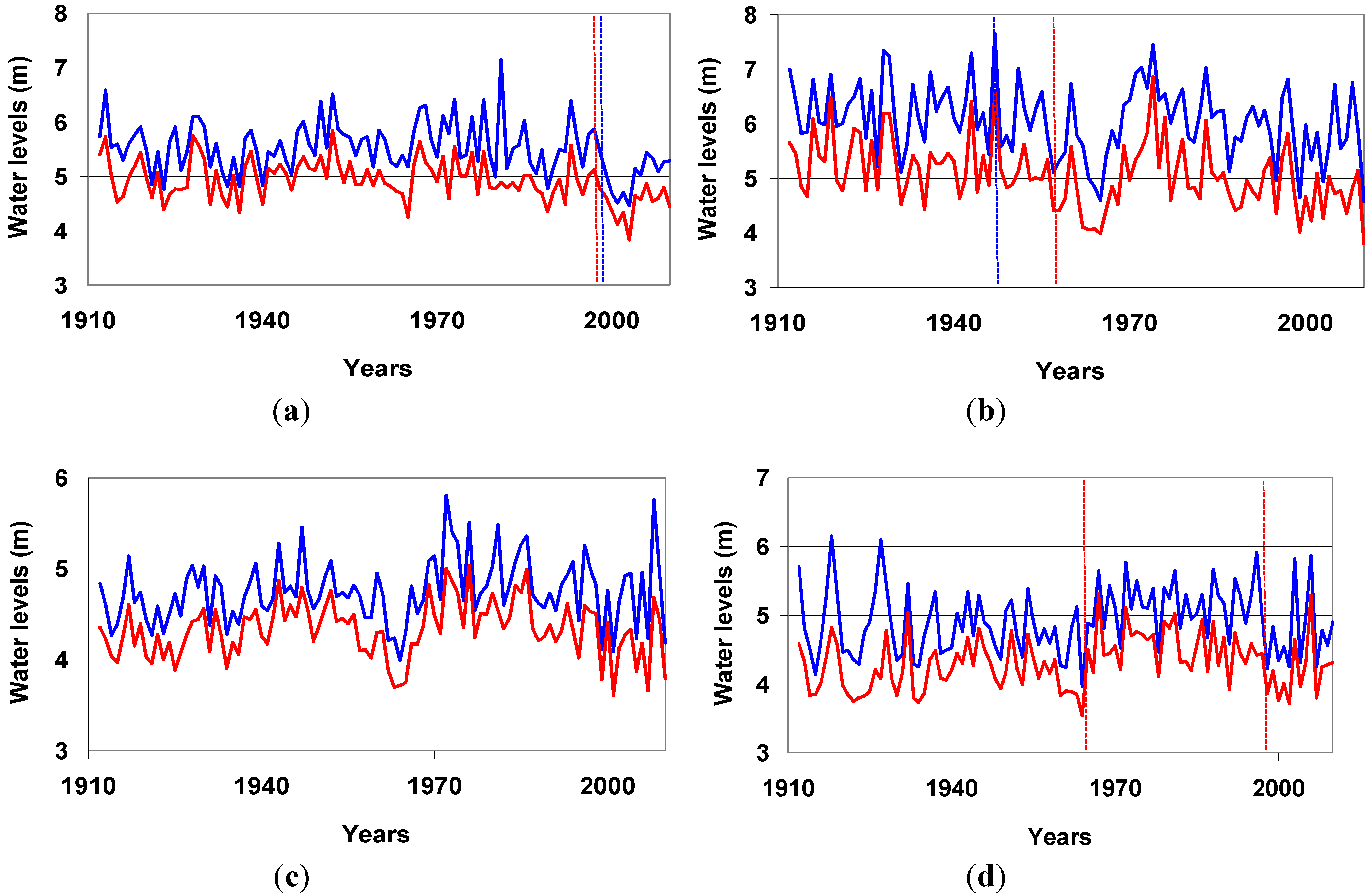
• Shifts in the mean values of a hydrological series may reflect site and/or measuring device changes over time. These two factors are excluded, because such changes do not apply to the Sorel station. Moreover, these types of changes will affect all monthly hydrological series, not only those for winter and spring. Finally, the dates of shifts produced by these types of changes should be synchronous for all hydrological variables and every month of the year.
• The effect of Lake Ontario. The St. Lawrence River is the main direct natural outlet for Lake Ontario and, indirectly, for the other North American Great Lakes. It is therefore reasonable to assign shifts in water levels in the St. Lawrence to shifts in water levels in Lake Ontario. However, a recent study [12] showed the absence of any synchronism between the temporal variability of annual daily extreme water levels in Lake Ontario and in the St. Lawrence River over the period from 1918 to 2010. Shifts in the mean values of water levels in Lake Ontario occurred much earlier than shifts in the mean water levels in the St. Lawrence River and are linked to the Great Drought of the 1930s. Based on these results, the study [12] concluded that the temporal variability of water levels in the St. Lawrence River at the Sorel station is affected much more strongly by water inputs from tributaries of the St. Lawrence than by those from Lake Ontario. Thus, shifts in the mean values of water levels in the St. Lawrence River cannot be assigned to a Lake Ontario effect.
• Regulation of water levels in the St. Lawrence River by dams and locks. Over the period from 1912 to 2010, a seaway channel was dug during the second half of the 1950s. This required the construction of numerous locks and dams, the largest of which, the Moses-Sanders dam, was built in the early 1960s to regulate water levels in the St. Lawrence. Such works may cause shifts in the mean values of hydrological series over time. Based on the timing of shifts in the mean constrained using the Lombard method, shifts that took place in the months of April and May (aside from shifts in minimum extreme water levels in May) can be assigned to digging of the seaway channel. The same goes for shifts in the mean values of maximum water levels observed in October and in minimum water levels observed in November and December, which can be linked to dam construction in the 1960s.
• Deforestation. Over the period from 1912 to 2010, the St. Lawrence River watershed was the site of deforestation associated with the industrial and economic development of North America during the last century. While no data are available to quantify the extent of this phenomenon in the St. Lawrence River watershed, the impacts of deforestation on streamflow in North American rivers are well-known. Numerous studies (e.g., [29,30,31]) have shown that deforestation induces an increase in extreme minimum streamflow and, to a lesser extent, in extreme maximum flows. Such changes are different from those observed in winter and spring minimum and maximum water levels in the St. Lawrence River, which decrease significantly over time. Thus, deforestation may be excluded as the cause of shifts in winter and springtime mean values. Additionally, given the lack of quantitative data on the evolution of the extent of deforestation in the St. Lawrence River watershed, which covers various temperate bioclimate regions, it is scientifically impossible to link the dates of shifts in the mean values with deforestation. Finally, the hydrological effects of deforestation should also be observed in summer and fall.
• Agriculture. Unlike deforestation, agriculture induces a decrease in extreme minimum flows without affecting extreme maximum flows in the St. Lawrence River watershed in Quebec, as shown in [32], which focuses on springtime and summer flows. Enhanced development of industrial farming in this watershed goes back to the 1960s. It is therefore difficult to link the shifts in winter minimum water levels that took place after the 1970s with agriculture. Furthermore, farming is restricted to the narrow alluvial plain that lines the St. Lawrence River and accounts for less than 1% of the overall aerial extent of its watershed. This, combined with the fact that farming is generally concentrated near the confluence of tributaries, suggests that agriculture is unlikely to be the sole factor accounting for shifts in the mean values of minimum and maximum extreme water levels in winter and spring. Finally, as for deforestation, the hydrological effects of agriculture should also be observable in summer.
• Urban development. The 20th century was a time of intense urban development in the St. Lawrence River watershed as a result of the industrial and economic development in the Great Lakes region. As for agriculture, this phenomenon is restricted to the narrow St. Lawrence River alluvial plain, where conditions lend themselves to farming and industrial development. Thus, the spatial extent of urban development is very limited in the St. Lawrence watershed. From a hydrological standpoint, it is also a well-known fact that the impacts of urban development usually produce increases in maximum flows (enhanced runoff) and decreases in minimum flows (decreased infiltration). In addition, urban development affects maximum flows more strongly than minimum flows. The demonstrated significant decrease in maximum water levels is therefore inconsistent with the effects of urban development. As far as minimum water levels are concerned, it would be difficult to link the observed shifts in the mean values to urban development, given the negligible spatial extent of this phenomenon in the whole watershed.
• Temperature. Many studies have demonstrated an increase in temperature in southern Canada in general and southern Quebec in particular (e.g., [9,11,33,34]). These studies showed that this warming was greater for winter than for other seasons. Such winter warming may have impacts on the temporal variability of water levels, as discussed below.

  -

  Warming temperatures can promote water evaporation and snow sublimation, leading to decreased springtime runoff. This can contribute to decreases in springtime maximum and minimum water levels. However, increased evaporation and/or snow sublimation would only have a limited impact on the temporal variability of maximum and minimum water levels in the winter. In addition, winter warming affects nighttime (minimum) temperatures much more strongly than daytime (maximum) temperatures. As a result, the effects of this nighttime warming on evaporation and snow sublimation are limited.

  -

  Increased winter temperatures promote the early melting of snow in the winter and spring (e.g., [7,33]). However, the effects of early snowmelt should lead to increased maximum and minimum water levels in March (winter) and April (spring). Therefore, this factor cannot account for the observed shifts.

  -

  Increased summer temperatures associated with a decrease in summer and fall rainfall. As aquifers are fed by summer and early fall rains, their decrease, combined with increasing summer temperatures, would lead to high evapotranspiration and, in turn, lower aquifer recharge in the summer and fall. If summer and fall rain is not sufficient to compensate for water losses in aquifers due to evapotranspiration, water levels, or minimum flows, in particular, will decrease in the fall and winter as a result of the limited amount of water supplied by aquifers. In their study, [9] observed a decrease in rainfall linked with increased summer temperatures.

• The amount of rain. Many studies have shown that the amount of winter rain has increased significantly in southern Quebec and southern Canada (e.g., [11,34,35]). While this increase only affects low-intensity rain events [11], any increase in the amount of rain should lead to an increase in maximum and minimum water levels in the winter. However, these water levels are observed to decrease over time. Even taking into account increased evaporation, which would still be low in the winter, increased rainfall in the winter cannot account for decreased water levels. In addition, as already mentioned, a decrease in rainfall in the summer and fall can affect aquifer recharge and, consequently, lead to decreased minimum water levels in the fall and winter.
• The amount of snow. Many studies have highlighted a significant decrease in snow accumulations in southern Canada and Quebec (e.g., [9,10,11,34]), which took place after the 1970s. Decreased snow accumulation can lead to a decrease in maximum and minimum extreme water levels in the fall, winter and springtime. Thus, as winter flow in the St. Lawrence River watershed in Quebec is mainly derived from aquifers, which are primarily recharged in springtime during snowmelt [36], a decrease in the amount of snow accumulated during the cold season (fall and winter) leads to limited aquifer recharge during spring snowmelt, resulting in lower streamflow during the following winter. Because springtime snowmelt is the main source of aquifer recharge in all Quebec watersheds, lower amounts of snow in the winter lead to a decrease in springtime maximum and minimum water levels in the St. Lawrence River, already strongly affected by flow regulation. However, this decrease in the amount of snow cannot account for the lack of synchronism between the shifts in the mean values in winter and spring, which could be due to the effect of other factors, such as temperature and water regulation by dams, which is not necessarily similar from month to month or season to season.

As far as the fall season is concerned, the first shifts in the mean took place during the 1960s, after construction of the Moses-Saunders dam. Thus, this dam could account for the significant increase in extreme minimum water levels in November and December, as well as in maximum water levels in October. It should be pointed out that the 1960s decade was a dry one for the south shore of the St. Lawrence River [37,38], and the increase in water levels observed in the fall is incompatible with this drought. As for the month of October, the increase in minimum water levels after 1936 cannot be linked to any known natural or human factor, nor can the drought that took place during that decade account for this increase. The second shift in the mean, which is only observed for extreme minimum water levels in November and December, took place after the 1970s. After this shift, and in contrast to what happened after the first shift, the mean values decreased significantly. This second shift may be linked to the decrease in the amount of snow in fall and winter and to increased evapotranspiration in summer and early fall.

Notwithstanding the asynchronous nature of the shifts in the long-term mean values observed for the different seasons, correlation analysis revealed that monthly daily maximum and minimum water levels are mainly negatively correlated with AMO, particularly in winter and spring. This correlation is also observed between AMO and annual daily maximum and minimum water levels [12] and for monthly mean water levels [14]. In North America, AMO is correlated negatively to precipitation and streamflow in a large part of the regions located within the continent (e.g., [39,40,41,42]). Negative anomalies of the climate index correspond with positive precipitation anomalies in interior North American. This relationship, however, is relatively complex, due to the effect of other factors on the temporal variability of water levels and streamflow. This accounts for the weak link (weak correlation) generally observed between climate indices and water levels (or flow) in streams. This being said, according to [42], AMO is the most consistent indicator of drought (decadal and multidecadal times scales) variability in the conterminous U.S. during the 20th century.

Finally, the study highlights the problem associated with selecting hydrological series and the scale of analysis for detecting the impacts of changes in the temperature and precipitation regimes on the temporal variability of water levels in the St. Lawrence River in a climate warming context. It is worth recalling that such a signal has not been detected in the variability of annual daily (maximum and minimum) extreme water levels [12], nor in the variability of annual mean water levels or streamflow [15], two series commonly analyzed in the scientific literature. Results from this study do, however, suggest that this signal was detected in a series of winter monthly daily extreme water levels. Thus, winter seems to be the best-suited season over which to track the impacts of climate warming on the temporal variability of water levels in the St. Lawrence River in Quebec.

5. Conclusions

Analysis of monthly daily extreme water levels (highest and lowest water levels measured for each month of each year) in the St. Lawrence River measured at the Sorel station since 1912 did not reveal any difference in the temporal variability of water levels in the St. Lawrence for the winter and spring. This variability is characterized by a significant decrease in the mean values of extreme water levels over time after the 1970s for the winter and fall, but before the 1970s for the spring. Before the 1970s, mean values of fall water levels increased significantly after their shifts. The decrease in daily extreme water levels is likely related to decreasing snowfall observed after the 1970s in the St. Lawrence River watershed in Quebec. In contrast, the decrease (springtime) and the increase (fall) in daily extreme water levels observed before the 1970s may be linked to the digging of the St. Lawrence Seaway and the construction of dams. Monthly daily extreme water levels for two seasons are generally correlated negatively with AMO. This study shows that the temporal variability of extreme water levels in the St. Lawrence River since 1912 was affected by climate variability (winter and fall) and human activity (spring and fall). The effects of these two factors are much greater on minimum than on maximum extreme water levels. As a result, minimum water levels appear to be the most appropriate hydrologic variable for monitoring the impacts of human activity and climate change on the temporal variability of water levels in the St. Lawrence River in Quebec. Finally, human activity and climate change must be considered when attempting to predict the temporal variability of extreme water levels in the St. Lawrence River using hydroclimatic models in the context of climate warming.

References

- Frenette, J.J.; Massicotte, P.; Lapierre, J.F. Colorful niches of phototrophic microorganisms shaped by the spatial connectivity in a large river ecosystem: a riverscape perspective. PLoS ONE 2012, 7, e35891. [Google Scholar]
- Boyer, C.; Chaumont, D.; Chartier, I.; Roy, A.G. Impact of climate change on the hydrology of St. Lawrence tributairies. J. Hydrol. 2010, 384, 65–83. [Google Scholar] [CrossRef]
- Hudon, C. Shift in wetland plant composition and biomass following low-level episodes in the St. Lawrence River: Looking into the future. Can. J. Fish. Aquat. Sci. 2004, 61, 603–617. [Google Scholar] [CrossRef]
- Hodgkins, G.A.; Dudley, R.W. Changes in the timing of winter-spring streamflows in eastern North America, 1912–2002. Geophys. Res. Lett. 2006, 33. [Google Scholar] [CrossRef]
- Burn, D.H. Climatic influences on streamflow timing in the headwaters of the Mackenzie River Basin. J. Hydrol. 2008, 352, 225–238. [Google Scholar] [CrossRef]
- Cayan, D.R.; Kammeriener, S.A.; Dettinger, M.D.; Caprio, J.M.; Peterson, D.H. Changes in the onset of spring in the western United States. Bull. Am. Meteorol. Soc. 2001, 82, 399–415. [Google Scholar] [CrossRef]
- Cunderlik, J.M.; Ouarda, B.M.J. Trend in the timing and magnitude of floods in Canada. J. Hydrol. 2009, 375, 471–480. [Google Scholar]
- Déry, S.J.; Stahl, K.; Moore, R.D.; Whitfield, P.H.; Menounos, B.; Burford, J.E. Detection of runoff timing changes in pluvial, nival and glacial rivers of western Canada. Water Resour. Res. 2009, 45. [Google Scholar] [CrossRef]
- Yagouti, A.; Boulet, G.; Vincent, L.; Vescovi, L.; Mékis, E. Observed changes in daily temperature and precipitation indices for southern Québec, 1960–2005. Atmosphere-Ocean 2008, 46, 243–256. [Google Scholar] [CrossRef]
- Brown, R.D. Analysis of snow cover variability and change in Québec, 1948–2005. Hydrol. Process. 2010, 24, 1929–1954. [Google Scholar]
- Vincent, L.A.; Mekis, E. Changes in daily and extreme temperature and precipitation indices for Canada over the twentieth century. Atmosphere-Ocean 2006, 44, 177–193. [Google Scholar] [CrossRef]
- Assani, A.A.; Landry, R.; Biron, S.; Frenette, J.J. Analysis of the interannual variability of annual daily extreme water levels in the St Lawrence River and Lake Ontario from 1918 to 2010. Hydrol. Process. 2013. [Google Scholar] [CrossRef]
- Hudon, C. Impact of water level fluctuations on St. Lawrence River aquatic vegetation. Can. J. Fish. Aquat. Sci. 1997, 54, 2853–2865. [Google Scholar] [CrossRef]
- Massicotte, P.; Assani, A.A.; Gratton, D.; Frenette, J.J. Relationship between water color, water levels, and climate indices in large rivers: Case of the St. Lawrence River (Canada). Water Resourc. Res. 2013, 49, 2303–2307. [Google Scholar] [CrossRef]
- McBean, E.; Motiee, H. Assessment of impact of climate change on water resources: A long term analysis of the Great Lakes of North America. Hydrol. Earth Syst. Sci. 2008, 12, 239–255. [Google Scholar] [CrossRef]
- Morin, J.; Leclerc, M. From pristine to present state: Hydrology evolution of Lake Saint-François, St. Lawrence River. Can. J. Civ. Eng. 1998, 25, 864–879. [Google Scholar] [CrossRef]
- Assani, A.A.; Stichelbout, E.; Roy, A.G.; Petit, F. Comparison of impacts of dams on the annual maximum flow characteristics in three regulated hydrological regimes in Québec (Canada). Hydrol. Process. 2006, 20, 3485–3501. [Google Scholar] [CrossRef]
- Lajoie, F.; Assani, A.A.; Roy, A.G.; Mesfioui, M. Impacts of dams on monthly flow characteristics. The influence of watershed size and seasons. J. Hydrol. 2007, 334, 423–439. [Google Scholar] [CrossRef]
- Matteau, M.; Assani, A.A.; Mesfioui, M. Application of multivariate statistical analysis methods to the dam hydrologic impact studies. J. Hydrol. 2009, 371, 120–128. [Google Scholar] [CrossRef]
- Vadnais, M.E.; Assani, A.A.; Landry, R.; Leroux, D.; Gratton, D. Analysis of the effects of human activities on the hydromorphological evolution channel of the Saint-Maurice River downstream from La Gabelle dam (Quebec, Canada). Geomorphology 2012, 175–176, 199–208. [Google Scholar] [CrossRef]
- Environment Canada Web Page. Données hydrométriques. Available online: http://www.wsc.ec.gc.ca/applications/H2O/index-fra.cfm (accessed on 20 March 2011).
- Lombard, F. Rank tests for changepoint problems. Biometrika 1987, 74, 615–624. [Google Scholar]
- Quessy, J.F.; Favre, A.C.; Saïd, M.; Champagne, M. Statistical inference in Lombard’s smooth-change model. Environmetrics 2011, 22, 882–893. [Google Scholar] [CrossRef]
- Von-Storch, H.; Navarra, A. Analysis of Climate Variability; Springer: New York, NY, USA, 1995. [Google Scholar]
- Önöz, B.; Bayazit, M. Block bootstrap for Mann-Kendall trend test of serially dependent data. Hydrol. Process. 2012, 26, 3552–3560. [Google Scholar] [CrossRef]
- National Oceanic and Atmospheric Administration Web Page. Climate Indices Data. Available online: http://www.esrl.noaa.gov/psd/data/climateindices/list/ (accessed on 10 June 2006).
- The National Center for Atmospheric Research Web Page. Climate Indices Data. Available online: http://www.cgd.ucar.edu/cas/jhurrell/indices.data.html (accessed on 10 August 2006).
- Joint Institute for the Study of Atmosphere and Ocean Page Web. Climate Indices Data. Available online: http://jisao.washington.edu/data/ao/ (accessed on 10 June 2006).
- Caissie, D.; Jolicoeur, S.; Bouchard, M.; Poncet, E. Comparison of streamflow between pre and post timber harvesting in Catamaran Brook (Canada). J. Hydrol. 2002, 258, 232–248. [Google Scholar] [CrossRef]
- Hornbeck, J.W.; Pierce, R.S.; Federer, C.A. Streamflow changes after forest clearing in New England. Water Resour. Res. 1970, 6, 1124–1132. [Google Scholar] [CrossRef]
- Lavigne, M.-P.; Rousseau, A.N.; Turcotte, R.; Laroche, A.-M.; Fortin, J.-P.; Villeneuve, J.-P. Validation and use of a semidistributed hydrological modelling system to predict short-term effects of clear-cutting on a watershed hydrological regime. Earth Interact. 2004, 8, 1–19. [Google Scholar]
- Muma, M.; Assani, A.A.; Landry, R.; Quessy, J.-F.; Mesfioui, M. Effects of the change from forest to agriculture land use on the spatial variability of summer extreme daily flow characteristics in southern Quebec (Canada). J. Hydrol. 2011, 407, 153–163. [Google Scholar]
- Adamowski, J.; Adamowski, K.; Prokoph, A. Quantifying the spatial temporal variability of annual streamflow and meteorological changes in eastern Ontario and southwestern Quebec using wavelet analysis and GIS. J. Hydrol. 2013, 499, 27–40. [Google Scholar]
- Zhang, X.; Vincent, L.A.; Hogg, W.D.; Niitso, A. Temperature and precipitation in Canada during the 20th century. Atmosphere-Ocean 2000, 38, 395–429. [Google Scholar] [CrossRef]
- Groleau, A.; Mailhot, A.; Talbot, G. Trend analysis of winter rainfall over southern Québec and New brunswick (Canada). Atmosphere-Ocean 2007, 45, 153–162. [Google Scholar] [CrossRef]
- Larocque, M.; Pharand, M.C. Dynamique de l’écoulement souterrain et vulnérabilité d’un aquifère du piedmont appalachien (Québec, Canada). Rev. Sci. Eau. 2010, 23, 73–88. [Google Scholar]
- Bradbury, J.A.; Dingman, S.L.; Barry, D.K. New England drought and relations with large scale atmospheric circulation patterns. J. Am. Water Res. Ass. 2002, 38, 1287–1299. [Google Scholar] [CrossRef]
- Assani, A.A.; Landais, D.; Mesfioui, M.; Matteau, M. Relationship between an Atlantic multidecadal oscillation index and variability of mean annual flows for catchments in the St. Lawrence watershed (Québec, Canada) during the past century. Hydrol. Res. 2010, 41, 115–125. [Google Scholar] [CrossRef]
- Curtis, S. The Atlantic multidecadal oscillation and extreme daily precipitation over the US and Mexico during the Hurricane season. Clim. Dyn. 2008, 30, 343–351. [Google Scholar] [CrossRef]
- Enfield, D.B.; Mestas-Nunez, A.; Trimble, P.J. The Atlantic multidecadal oscillation and its relation to rainfall and river flows in the continental US. Geophys. Res. Lett. 2001, 28, 2077–2080. [Google Scholar] [CrossRef]
- McCabe, G.J.; Palecki, M.A.; Betancourt, J.L. Pacific and Atlantic Ocean influences on multidecadal drought frequency in the United States. Proc. Natl. Acad. Sci. USA 2004, 101, 4136–4141. [Google Scholar] [CrossRef]
- McCabe, G.J.; Betancourt, J.L.; Gray, S.T.; Palecki, M.A.; Hidalgo, H.G. Associations of multi-decadal sea-surface temperature variability with US drought. Quatern. Intern. 2008, 188, 31–40. [Google Scholar] [CrossRef]
© 2014 by the authors; licensee MDPI, Basel, Switzerland. This article is an open access article distributed under the terms and conditions of the Creative Commons Attribution license (http://creativecommons.org/licenses/by/3.0/).
Share and Cite
Assani, A.; Landry, R.; Labrèche, M.; Frenette, J.-J.; Gratton, D. Temporal Variability of Monthly Daily Extreme Water Levels in the St. Lawrence River at the Sorel Station from 1912 to 2010. Water 2014, 6, 196-212. https://doi.org/10.3390/w6020196
Assani A, Landry R, Labrèche M, Frenette J-J, Gratton D. Temporal Variability of Monthly Daily Extreme Water Levels in the St. Lawrence River at the Sorel Station from 1912 to 2010. Water. 2014; 6(2):196-212. https://doi.org/10.3390/w6020196
Chicago/Turabian StyleAssani, Ali, Raphaëlle Landry, Mikaël Labrèche, Jean-Jacques Frenette, and Denis Gratton. 2014. "Temporal Variability of Monthly Daily Extreme Water Levels in the St. Lawrence River at the Sorel Station from 1912 to 2010" Water 6, no. 2: 196-212. https://doi.org/10.3390/w6020196
APA StyleAssani, A., Landry, R., Labrèche, M., Frenette, J.-J., & Gratton, D. (2014). Temporal Variability of Monthly Daily Extreme Water Levels in the St. Lawrence River at the Sorel Station from 1912 to 2010. Water, 6(2), 196-212. https://doi.org/10.3390/w6020196