Integration of a Hydrological Model within a Geographical Information System: Application to a Forest Watershed

Abstract

Watershed simulation software used for operational purposes must possess both dependability of results and flexibility in parameter selection and testing. The UBC watershed model (UBCWM) contains a wide spectrum of parameters expressing meteorological, geological, as well as ecological watershed characteristics. The hydrological model was coupled to the MapInfo GIS and the software created was named Watershed Mapper (WM). WM is endowed with several features permitting operational utilization. These include input data and basin geometry visualization, land use/cover and soil simulation, exporting of statistical results and thematic maps and interactive variation of disputed parameters. For the application of WM two hypothetical scenarios of forest fires were examined in a study watershed. Four major rainfall events were selected from 12-year daily precipitation data and the corresponding peak flows were estimated for the base line data and hypothetical scenarios. A significant increase was observed as an impact of forest fires on peak flows. Due to its flexibility the combined tool described herein may be utilized in modeling long-term hydrological changes in the context of unsteady hydrological analyses.

1. Introduction

The objective of Operational Hydrology is to control the operation of water systems and to provide aid in dealing with problems of water use and water management. Watershed simulation software used for operational purposes must possess both dependability of results and flexibility in parameter selection and testing.

The UBC watershed model (UBCWM), created initially at the University of British Columbia [1], has been extensively applied and tested in watersheds around the world, under a great variety of climatic conditions and physiographic characteristics [2,3,4]. Also, it contains a wide spectrum of parameters expressing meteorological, geological, as well as ecological watershed characteristics.

However, UBCWM lacks spatial functionality both for input data and outputs. The objective of this study was the development of software which would improve the facility and the flexibility of the use of UBCWM. The UBCWM source code has been recently rewritten in a Visual Basic 6 environment and subsequently the hydrological model was coupled to MapInfo GIS, via a code written in MapBasic, the programming language associated to MapInfo. The software thus created was named Watershed Mapper (WM) for UBCWM (UBCWM + WM). WM is endowed with several features permitting full operational utilization. These include input data and basin geometry visualization, exporting of statistical results and thematic maps, and interactive variation of disputed parameters.

Possible scenarios of land cover changes, due to forest fires for instance, can be introduced into the UBCWM+WM and their effect can be evaluated on the hydrology of the watershed. Related sensitivity studies can also be carried out. The impacts on land cover changes can easily be evaluated and facilitate decision making.

More generally, the UBCWM + WM may be utilized in unsteady hydrological modeling, such as detection of trends or changes in hydrologic time series that are due to changing conditions in the studied watershed.

2. The UBC Watershed Model

The UBCWM was first presented 25 years ago [5], and has been updated continuously to its present form. The UBCWM is a continuous conceptual hydrologic model which accepts input and calculates water balance components in a semi-distributed way but calculates the runoff from the flow components through lumped routing. It operates in hourly and/or daily time step using precipitation, maximum and minimum temperature as input data from a number of stations. It was designed for the simulation of streamflow from mountainous watersheds, where the runoff from snowmelt and glacier melt may be important, apart from the rainfall runoff. However, the UBCWM has been applied to a variety of climatic regions, ranging from coastal to inland mountain regions of British Columbia including the Rocky Mountains, and the subarctic region of Canada [1,3,4,6,7,8]. The model has also been applied to the Himalayas and Karakoram Mountain Ranges in India and Pakistan, the Southern Alps in New Zealand and the Snowy Mountains in Australia [9]. This ensures that the model is capable of simulating runoff under a large variety of conditions.

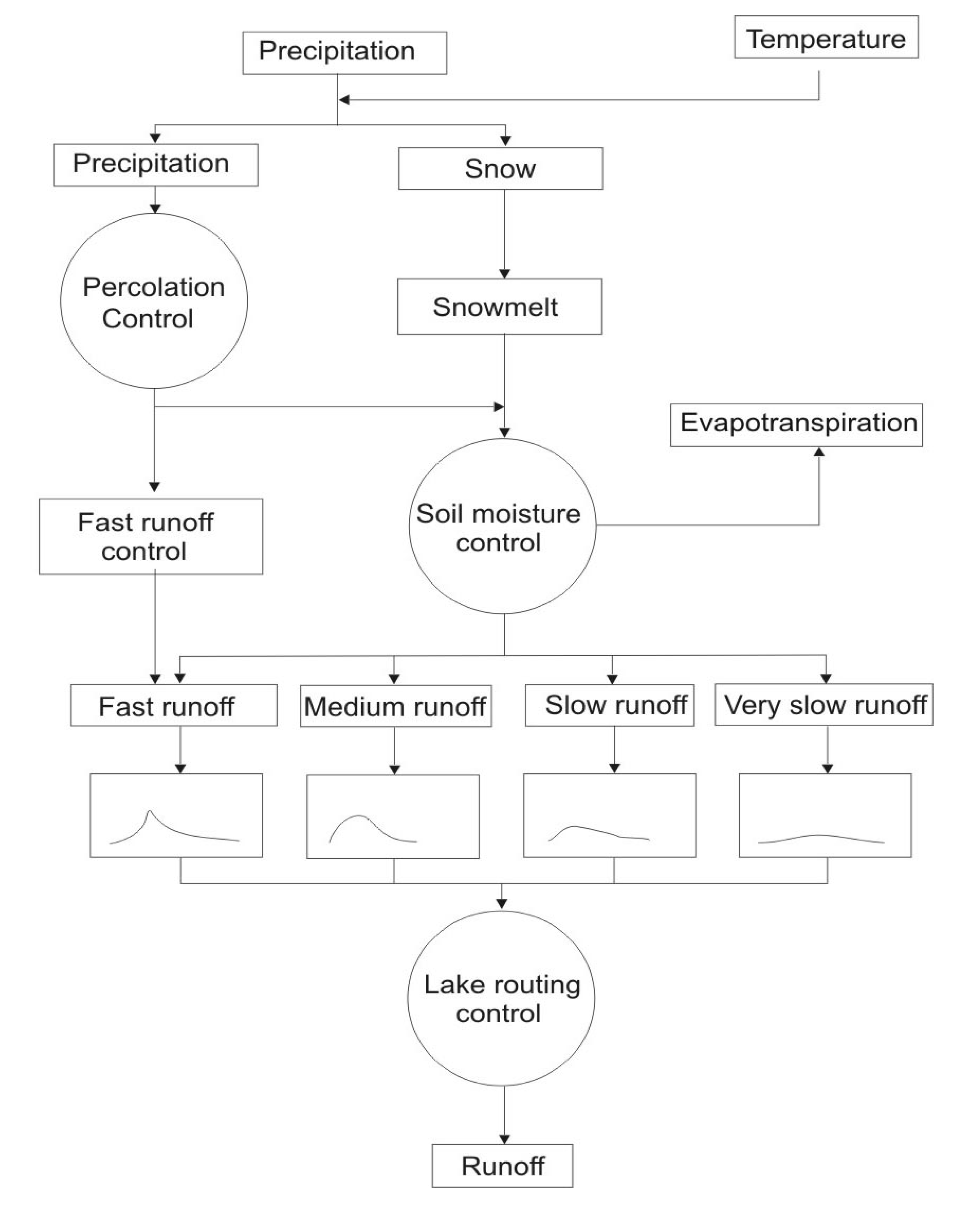
In general, the meteorological data base is sparse for most of the mountainous regions modeled. In the majority of situations, the meteorological data is from valley stations. As a result of these data constraints, an important aspect of the UBCWM is the elevation distribution of data. Functional relationships are specified describing the variability of temperature lapse rates. The temperature lapse rate is a key relationship because it influences the precipitation distribution, and it is also very significant in determining snowmelt rates at various elevations. Precipitation inputs are made functionally dependent on elevation and on temperature regime. This functional variation of precipitation automatically recognizes that precipitation undergoes greater orographic enhancement during the winter than it does during warm summer rainstorms. The general structure of the UBCWM is indicated in the flow chart, Figure 1.

Figure 1. The UBC watershed model (UBCWM) flow chart.

Figure 1. The UBC watershed model (UBCWM) flow chart.

Water is allocated to each of the components of runoff, namely fast, medium, slow and very slow, which are subjected to a routing procedure thus producing delays (time distribution runoff). The routing procedure for each component is based on the same underlying concept, namely the linear storage reservoir. The fast and medium components of runoff are subjected to a cascade of reservoirs which is essentially identical to unit hydrograph convolution. The lower components of runoff simply use a single linear reservoir, thus avoiding the necessity to convolute for the final outflow. The component flow routing calculation is based on a conceptual model of the runoff process developed by Nash [10] in which inflows are passed through a cascade of linear reservoirs. The resulting outflow at a time t from a unit impulse of inflow is:

(1)

where K is the linear storage constant for each of the reservoirs in the cascade; n is the number of linear reservoirs in the cascade; t is the time after the water input has occurred.

Three main steps, necessary for the application of UBCWM, are: (a) observation of historical meteorological and flow data of the watershed; (b) watershed description; (c) calibration of the parameters, so that the flow is conformed to the historical data. An input file is divided into 10 groups of parameters, each dealing with a particular aspect of the modeling process, providing the UBCWM with run control instructions and a physical description of a watershed, which determines how it responds to temperature and precipitation inputs. These groups are:

• Time and date run control;
• Meteorological and flow data;
• Elevations and parameters for meteorological stations;
• Description of the watershed;
• Distribution of meteorological variables;
• Snowmelt function;
• Water distribution;
• Initial conditions;
• Initial values of outflows from routing storages;
• Monthly parameters.

Some of these, such as the physical description of the watershed, must be modified for each watershed. Others, such as the snowmelt function variables, will rarely, if ever, be changed. The UBCWM has, in total, more than 90 parameters. However, application of the model to various climatic regions and experience have shown that only the values of 18 general parameters and two precipitation representation factors for each meteorological station have to be optimized and adjusted during calibration, and the majority of the parameters take standard constant values. These varying model parameters can be separated into three groups: the parameters that control precipitation distribution, the water allocation parameters, and the flow routing parameters.

The above model parameters are optimized through a two-stage procedure. At the first stage, a sensitivity analysis of each parameter is performed to estimate the range of parameter values for which the simulation results are the most sensitive. At the second stage, a Monte Carlo simulation is performed for each parameter of each group by keeping the parameters of the other two groups constant. The values of the parameters are sampled from the respective parameter range defined during the first stage of the procedure (sensitivity analysis). The parameter values that maximize the objective function are put in the parameter file and the procedure is repeated for the parameters of the next group. The procedure starts with the optimization of the precipitation distribution parameters and ends with the optimization of the flow routing parameters. The objective function of the above optimization procedure is defined as:

(2)

where, V_sim and V_obs are the simulated and the observed flow volumes, respectively and Eff is the Nash-Sutcliffe efficiency [11] defined as:

(3)

where, Qobs_i is the observed flow on day i; Qsim_i is the simulated flow on day i; Qobs is the average observed flow and n is the number of days for the simulation period.

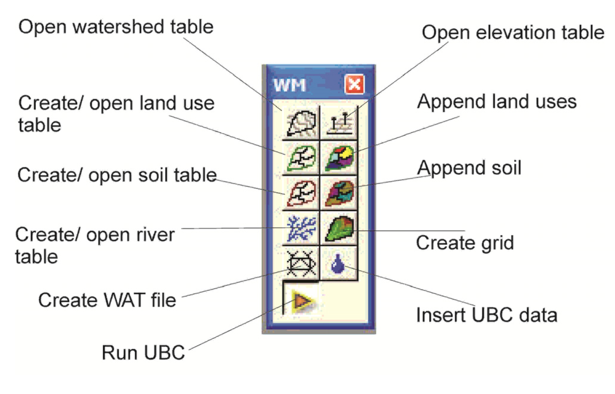
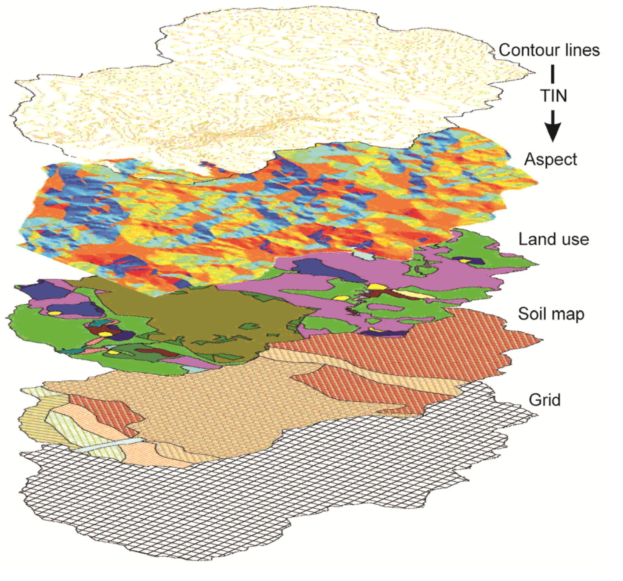
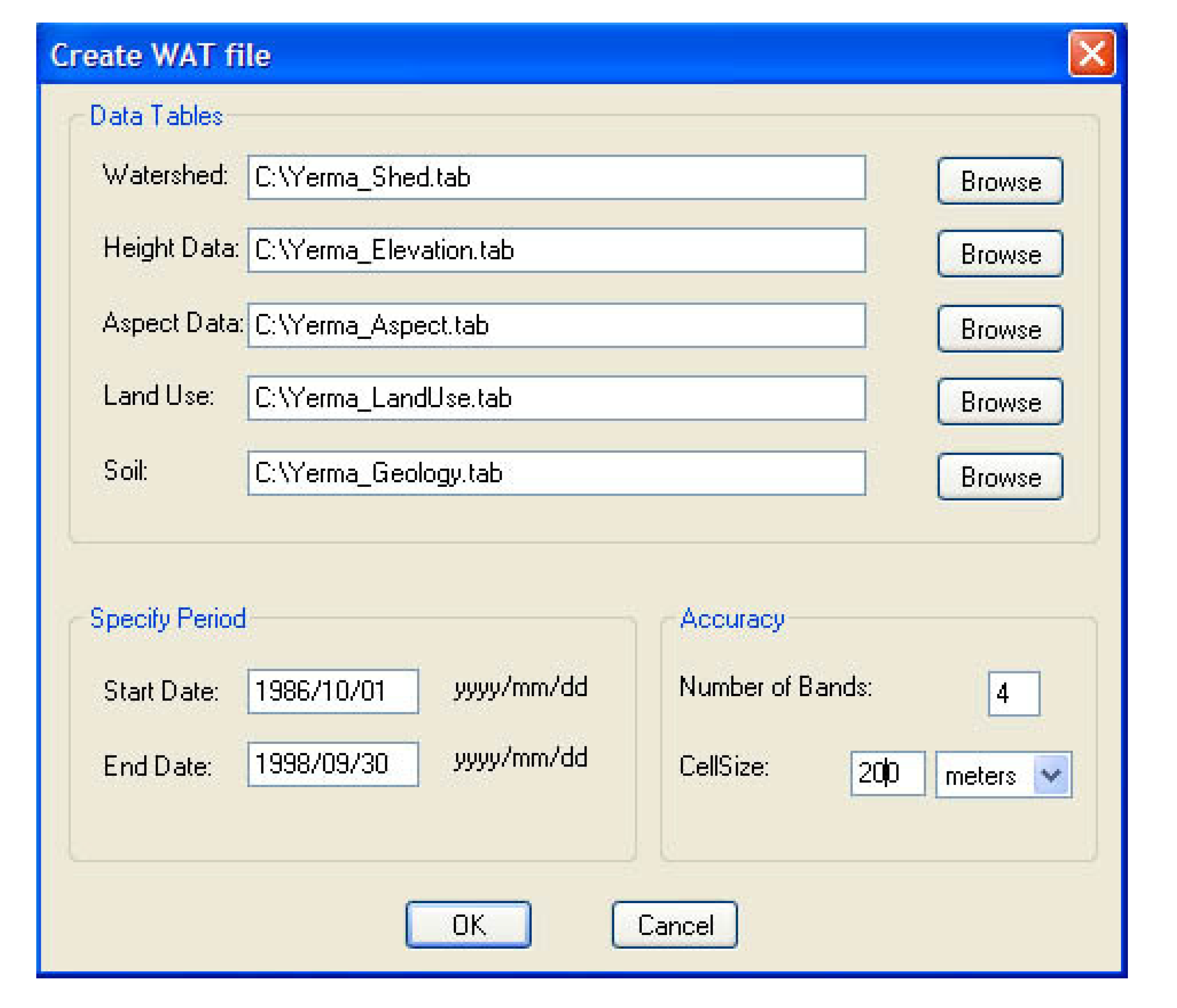
In order for UBCWM to run, water basin limits have to be defined and every basin needs to be compartmentalized in 1–12 elevation bands. Every band has to be informed with a number of physical parameters. The input of this information is a time consuming and tedious procedure. After model’s implementation, a set of variables and results are produced. Besides, outputs can be displayed in table format, but not in map format. This feature dispossesses spatial analysis and management of hydrologic procedures in a watershed, if UBCWM is employed alone. An accompanying geographic information system (GIS) can easily tackle these handicaps, as described in the next section. The object oriented nature of UBCWM (VB environment) opened the possibility for all the above parameters and features to be advantageously utilized by an external GIS.

3. Watershed Mapper

WM is embedded into GIS MapInfo Professional. It was created and developed with the help of MapBasic 6.5, the programming language of MapInfo Professional [12], and Visual Basic 6.0. It is a tool which allows the user to employ the UBCWM in the environment of MapInfo Professional by collecting, managing, analyzing, and displaying spatial and temporal inputs and outputs.

3.1. Communication with UBCWM

WM and UBCWM are two separate programs, which collaborate. The connection and collaboration were achieved with the help of Dynamic Data Exchange (DDE). DDE is a feature of Windows that allows two programs to share data or send commands directly to each other. DDE can be thought of as a direct conversation between two application programs.

DDE functions as a connector between an application that is the source of the data and is called the “server” and the application that is receiving the data and is called the “client”. In our case, the server application is the UBCWM and the client application is the WM. The client application begins the exchange establishing a “dialogue” with the server application by sending out commands. The “dialogue” starts with a request for data or operations. The server application responds by providing results to the client application. Finally, the UBCWM fully works in the MapInfo environment.

3.2. Watershed Mapper Interface

The WM structure can be divided into 3 main functions: (i) importing and processing of source data; (ii) running UBCWM; and (iii) displaying outputs. The implementation of these functions can be established from the pull-down menu or the button pad toolbar provided by WM (Figure 2)

Figure 2. Watershed Mapper button pad toolbar.

Figure 2. Watershed Mapper button pad toolbar.

3.2.1. Import and Processing of Source Data

Source data is the term for scanned maps, aerial photographs and satellite images used for input data such as watershed’s limits, heights, land use–land cover, geology and soil. WM builds a database and a grid for the proper distribution of these data layers. The size of the grid cells depends on source data accuracy and is defined by the user. Every cell of the watershed carries information on: (a) elevation; (b) north-south orientation; (c) impermeable fraction; (d) forested fraction and (e) forest canopy density coming from the above mentioned data layers (Figure 3). All this spatially distributed information as well as the start and end dates of runs are fed into the UBCWM choosing the respective files using a dialog box (Figure 4).

Figure 3. Data layers’ integration.

Figure 3. Data layers’ integration.

Figure 4. Appending data with watershed mapper.

Figure 4. Appending data with watershed mapper.

The fundamental component for the model to run is the parameter file. It is a text file which contains all the parameters needed, divided into 10 groups. WM allows the update of two groups of UBCWM parameters: (a) watershed description and (b) time run control. It also allows the running of UBCWM in MapInfo environment and finally, the extraction and the update of MapInfo’s Database.

Import and processing of source data function consisted of two components:

• Watershed Description. This section of the parameter file describes the physical characteristics of the watershed. The information is specific to each watershed and it is usually derived from the analysis of topographical maps and aerial photographs. For each elevation band these parameters give information about the mean elevation, mean area, forested fraction of the band, the density of the forest canopy, north-south orientation, glaciated area of the band, the fraction of any glacier with south orientation, the impermeable fraction of band, precipitation adjustment, and station temperature, precipitation and evapotranspiration indices. Table 1 shows how the watershed description parameters are generated in WM and UBCWM.
• Time and Date Run Control. This section contains parameters which control the start and end dates of runs.

3.2.2. UBCWM Implementation

UBCWM implementation is accomplished with the corresponding command. Certain changes in UBCWM’s VB code have been made and DDE undertakes to display and make operative all the forms and dialog boxes in MapInfo’s environment. Thereby, the user can deploy all UBCWM’s functions like run, optimization, statistics, hydrographs, etc.

Table 1. Watershed description parameters and meteorological data distribution for elevation bands and how they are spatially distributed.

Elevation band parameters	Necessary file	Spatially distributed by
mean elevation	contour lines map *	WM
mean area	watershed map	WM
forested fraction	land use map	WM
forest canopy density	land use map	WM
north-south orientation	contour lines map *	WM
glaciated area	glaciated area map	WM
glacier fraction south orientated	glaciated area map	WM
impermeable fraction	land use and soil map	WM
precipitation adjustment	meteorological stations map and data	WM and UBCWM
temperature	meteorological stations data	UBCWM **
precipitation	meteorological stations data	UBCWM **
evapotranspiration	meteorological stations data	UBCWM ***

Notes: * contour lines map produce an aspect map after a Triangulated Irregular Network (TIN) interpolation; ** using mean elevation parameter; *** using mean elevation and forest canopy density parameters.

Table 1. Watershed description parameters and meteorological data distribution for elevation bands and how they are spatially distributed.

Elevation band parameters	Necessary file	Spatially distributed by
mean elevation	contour lines map *	WM
mean area	watershed map	WM
forested fraction	land use map	WM
forest canopy density	land use map	WM
north-south orientation	contour lines map *	WM
glaciated area	glaciated area map	WM
glacier fraction south orientated	glaciated area map	WM
impermeable fraction	land use and soil map	WM
precipitation adjustment	meteorological stations map and data	WM and UBCWM
temperature	meteorological stations data	UBCWM **
precipitation	meteorological stations data	UBCWM **
evapotranspiration	meteorological stations data	UBCWM ***

Notes: * contour lines map produce an aspect map after a Triangulated Irregular Network (TIN) interpolation; ** using mean elevation parameter; *** using mean elevation and forest canopy density parameters.

3.2.3. Displaying Outputs

The third function of the software is the procedure during which the UBCWM processing results are received by the WM and suitably displayed within the GIS environment.

Examples of UBCWM processing results are contained in the following twenty six (26) new fields: observed flow, calculated flow, difference flow, snowmelt outflow, glacial contribution, rainfall outflow, groundwater, solar radiation, albedo, snow cover area, potential evapotranspiration loss, cloud cover, snowpack water equivalent, maximum temperature, minimum temperature, interception, snowfall, rainfall, snowmelt, upper groundwater, deep zone groundwater, snowmelt interflow, rainfall interflow, snowmelt fastflow and rainfall fastflow. All the above fields automatically update GIS database for every elevation band of the basin (Figure 5).

Figure 5. UBC’s 26 output parameters for Germasogeia’s elevation band 1.

Figure 5. UBC’s 26 output parameters for Germasogeia’s elevation band 1.

The import of these fields into the GIS allows the user to take advantage of GIS features like SQL (Structured Query Language) questions, thematic maps, statistic reports, layouts etc.

4. Forest Fire Scenarios and Its Impact on Water Flows

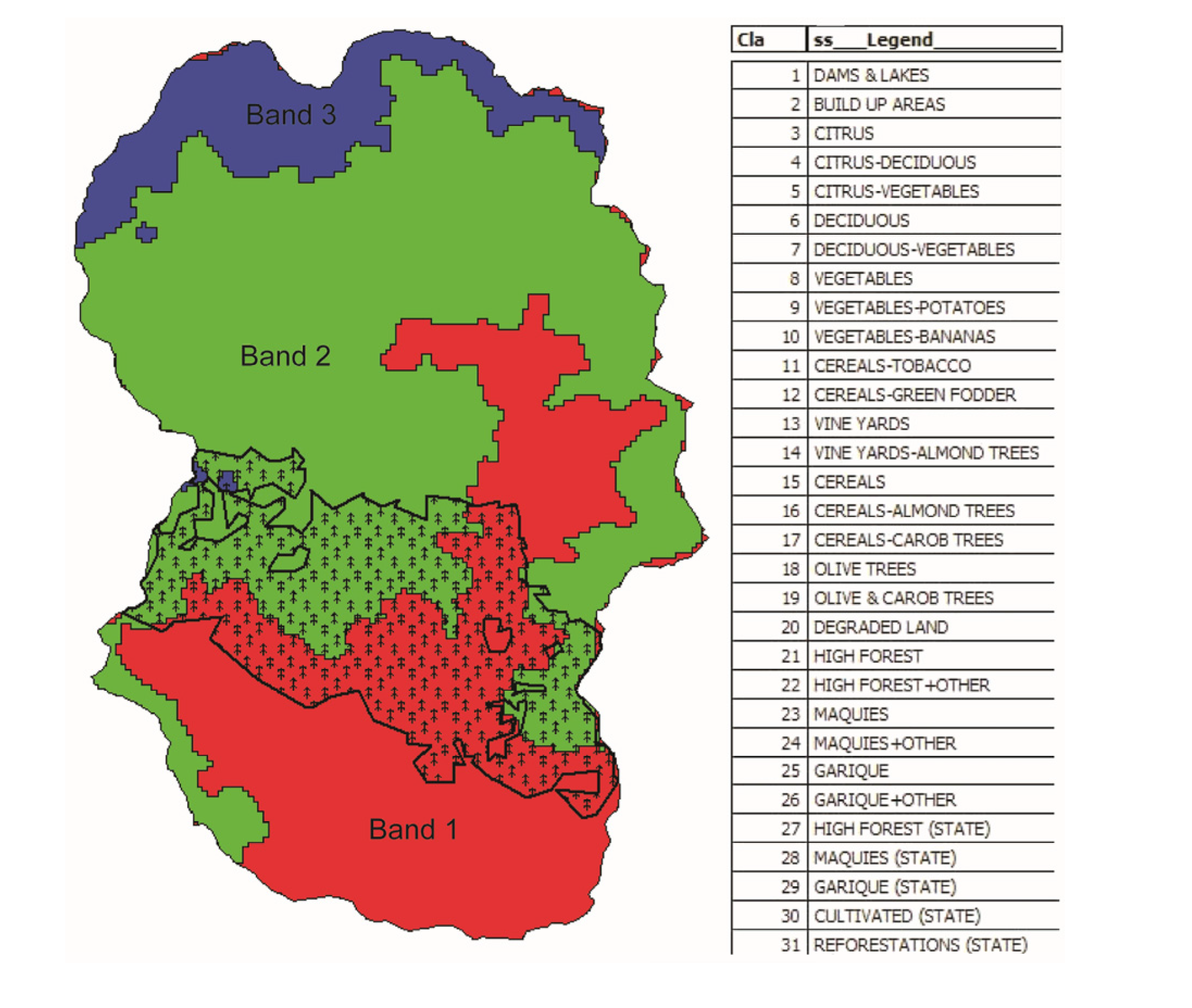
For the application of WM, the watershed of Germasogeia in Cyprus was selected. It is located at 34°49′ latitude, on the southern side of mountain Troodos of Cyprus, and roughly 5 km north of Limassol city. The watershed area is 160.4 km² and its elevation ranges from 70 m up to 1400 m. Most of the area is covered by typical Mediterranean type forest and sparse vegetation. A reservoir with storage capacity of 13.6 million m³ was constructed downstream the mouth of the watershed in 1969, for irrigation and municipal water supply purposes.

The climate of the area is a Mediterranean maritime climate with mild winters and hot and dry summers. The precipitation is usually generated by frontal weather systems moving eastwards. The average basin-wide annual precipitation is 640 mm, ranging from 450 mm at the low elevations up to 850 mm at the upper parts of the watershed. The mean annual runoff of Germasogeia River is about 150 mm, and 65% of it is generated by rainfall during winter months. The river is usually dry during summer months. The peak flows are observed in winter months and produced by rainfall events. The Germasogeia area is afflicted with problems of water scarcity. Land use and the extent of canopy affect significantly the hydrological regime of drainage basins [13,14,15]. Forest land occupies most of the Germasogeia watershed area dominating about 61% of the total land.

Forest fires are very common events in the Mediterranean type of ecosystems [16,17,18]. A recent forest fire on July 2007 endangered the forested area of mountain Troodos. In order to understand the potential impacts of a forest fire on the water regime in the Germasogeia basin, two hypothetical scenarios of forest fires are considered. According to the first scenario, about half of the area of the high forest (17 km²) located toward the south is destroyed by fire and the impact on the hydrological regime is evaluated. A second scenario involves the firing of the whole of the above forested area (about 34 km²). Both scenarios were examined for three rainfall events, and peak flows were calculated and compared. The entire watershed was divided into 2419 cells, with the size of each cell equal to 9 ha. Digital elevation data at a scale of 1:50,000 were used. Maps of the same scale were used for the extraction of soil, geological and land cover data. Good quality daily precipitation from three meteorological stations located at 70 m, 100 m, and 995 m of elevation were used. Data of maximum and minimum temperature measured at the low elevation station (70 m) were used in this study. In total, twelve years of meteorological and streamflow data (October 1986–September 1998) were available from the Germasogeia watershed. The UBCWM was calibrated using daily-recorded streamflow for the Germasogeia basin for the years 1986–1998. The statistics used to validate the performance of the model are the mean observed and the mean simulated flow, the coefficient of determination (r²), and the Nash-Sutcliffe efficiency (Eff) as defined above. Table 2 presents the flow comparison statistics for the calibration period of the model. The simulation/calibration period includes dry and wet years. The calibration results show that the Nash–Sutcliffe efficiency ranges from 0.60 to 0.94 and the coefficient of determination ranges from 0.68 to 0.94. Runoff statistics for wet and dry years indicate that the model is capable to reproduce the observed streamflow with accuracy. Four major rainfall events of the duodecennial were chosen and the respective peak flows were isolated and estimated for the hypothetic scenarios and compared to the undisturbed scenario (Table 3). The estimation of a watershed peak flood discharge magnitude is a fundamental parameter in hydrologic analysis, since it has been used in a variety of purposes such as the design of bridges, culverts, flood-control structures, as well as in the management and regulation of flood plains [19].

In simulating the effect of forest fires on fast runoff, this study assumed that the forest fraction and forest canopy were the only variables to be changed and other factors such as soil and topography remained the same. In reality, a forest fire often causes change in some related factors such as soil’s mechanical composition and percolation.

Table 2. Calibration statistics of the UBCWM.

Year	Mean observed flow (m3/s)	Mean simulated flow (m3/s)	Nash–Sutcliffe efficiency (Efficiency)	Coefficient of determination (r2)
1986	0.58	0.74	0.73	0.75
1987	0.77	0.62	0.71	0.75
1988	0.59	0.39	0.60	0.79
1989	0.17	0.27	0.63	0.81
1990	0.06	0.07	0.90	0.92
1991	0.65	0.69	0.73	0.77
1992	0.61	0.38	0.65	0.72
1993	0.29	0.21	0.74	0.76
1994	0.61	0.76	0.48	0.68
1995	0.16	0.13	0.73	0.81
1996	0.11	0.11	0.91	0.94
1997	0.08	0.07	0.94	0.94

Table 2. Calibration statistics of the UBCWM.

Year	Mean observed flow (m3/s)	Mean simulated flow (m3/s)	Nash–Sutcliffe efficiency (Efficiency)	Coefficient of determination (r2)
1986	0.58	0.74	0.73	0.75
1987	0.77	0.62	0.71	0.75
1988	0.59	0.39	0.60	0.79
1989	0.17	0.27	0.63	0.81
1990	0.06	0.07	0.90	0.92
1991	0.65	0.69	0.73	0.77
1992	0.61	0.38	0.65	0.72
1993	0.29	0.21	0.74	0.76
1994	0.61	0.76	0.48	0.68
1995	0.16	0.13	0.73	0.81
1996	0.11	0.11	0.91	0.94
1997	0.08	0.07	0.94	0.94

The WM was used to import and process input parameters and source data for UBCWM, to run UBCWM in MapInfo environment in order to produce estimates of fast outflows, and finally to display tabular and spatial outputs (Figure 5).

Table 3. Rainfall events and peak flows for two forest fires scenarios.

Date	Rainfall (mm)	Sum of undisturbed peak flow (m3/sec)	1st Scenario sum of peak flow (m3/sec)	Increase percentage	2nd Scenario sum of peak flow (m3/sec)	Increase percentage
03–22 March 1987	148	89	100	13	110	35
07–13 January 1989	88	40	46	16	51	28
20 December 1991–03 January 1992	123	64	75	17	79	23
17–24 November 1994	202	100	109	9	117	16

Table 3. Rainfall events and peak flows for two forest fires scenarios.

Date	Rainfall (mm)	Sum of undisturbed peak flow (m3/sec)	1st Scenario sum of peak flow (m3/sec)	Increase percentage	2nd Scenario sum of peak flow (m3/sec)	Increase percentage
03–22 March 1987	148	89	100	13	110	35
07–13 January 1989	88	40	46	16	51	28
20 December 1991–03 January 1992	123	64	75	17	79	23
17–24 November 1994	202	100	109	9	117	16

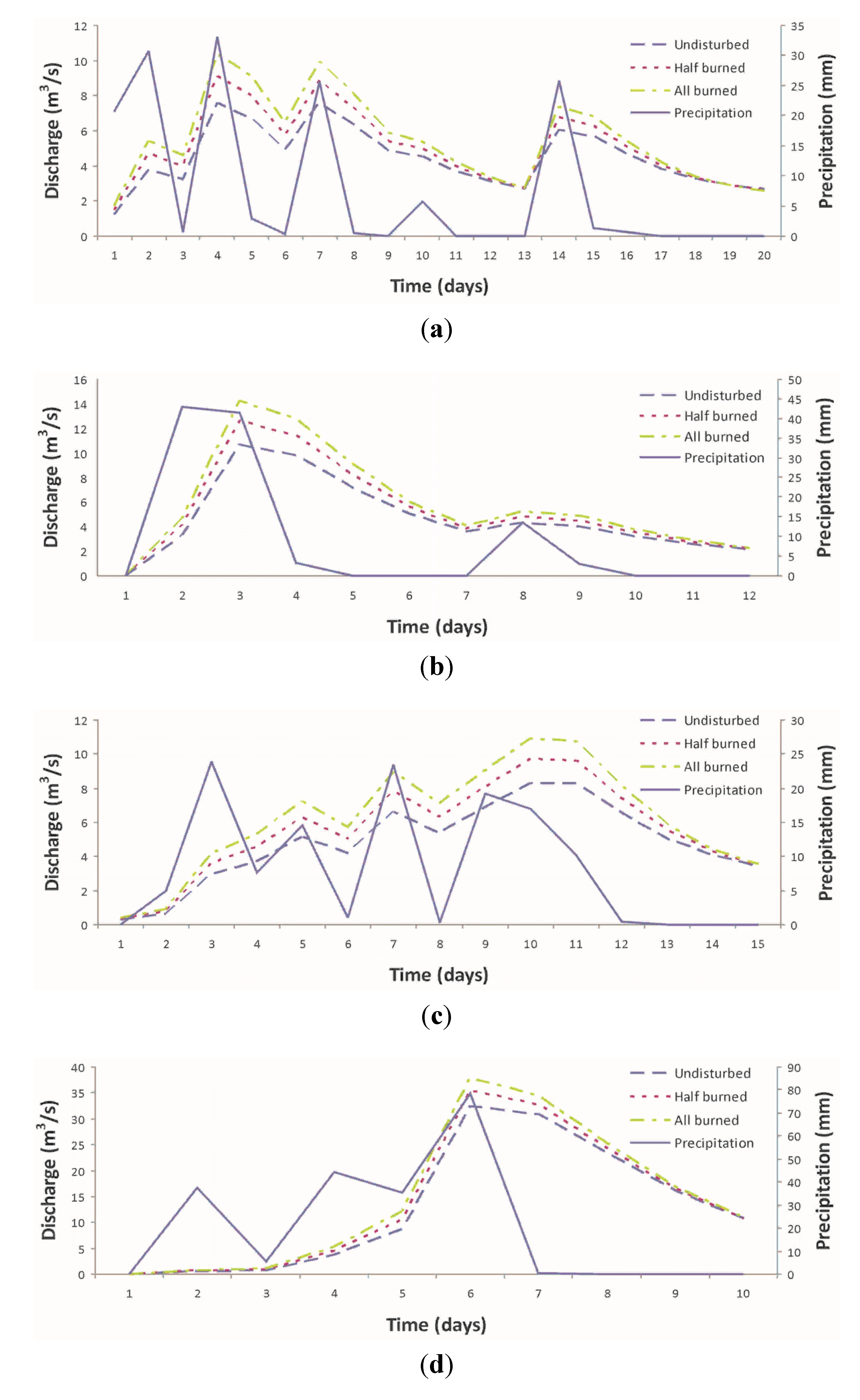
Figure 6 shows the peak flows in m³ for the three scenarios and the precipitation of three rainfall events. There is a respective increase of peak flows regarding burned forest area. Figure 7 shows the percentage of peak flow increase for the two hypothetic scenarios and the precipitation of the three events. As it can be seen, the increase in percentage is almost double for the “all burned” scenarios compared to the “undisturbed” scenarios.

Figure 6. Precipitation and peak flows of the four major rainfall events. (a) 3–22 March 1987; (b) 7–18 January 1989; (c) 20 December 1991–3 January 1992; (d) 17–26 November 1994.

Figure 6. Precipitation and peak flows of the four major rainfall events. (a) 3–22 March 1987; (b) 7–18 January 1989; (c) 20 December 1991–3 January 1992; (d) 17–26 November 1994.

These differences are due to the reduction of forested area and the impact in the three related parameters: Impermeable, forested fraction and forest canopy density. Significant changes are also noted in the runoff components, namely surface and ground water runoff (Table 4). Surface runoff is expressed through fast and medium components while ground water is expressed through slow and very slow components, as explained above. The absence of the forest results in a decrease of percolation, increasing fast and medium runoff. The biggest differences are observed in the 1st and 2nd elevation band, where the forest is occurred (Figure 5). Ground water decrease reached 17% in one case, while surface runoff increased 43% in another.

Figure 7. Peak flow increase percentage for the two hypothetic scenarios and the precipitation of the four major rainfall events. (a) 3–22 March 1987; (b) 7–18 January 1989; (c) 20 December 1991–3 January 1992; (d) 17–26 November 1994.

Figure 7. Peak flow increase percentage for the two hypothetic scenarios and the precipitation of the four major rainfall events. (a) 3–22 March 1987; (b) 7–18 January 1989; (c) 20 December 1991–3 January 1992; (d) 17–26 November 1994.

Table 4. Runoff components changes for two forest fire scenarios (a and b for ground (slow and very slow) and surface (fast and medium) water runoff components, respectively).

Date	03–22 March 1987		07–13 January 1989		20 December 1991–03 January 1992		17–24 November 1994
Rainfall	148 mm		88 mm		123 mm		202 mm
	Runoff components (m3/s) for the undisturbed forest
	a	b	a	b	a	b	a	b
1st Band	40	18	21	12	42	17	34	46
2nd Band	72	23	40	17	70	22	58	66
3rd Band	17	4	9	3	14	4	11	11
	Runoff components (m3/s) for the half forest burned (1st scenario)
	a	b	a	b	a	b	a	b
1st Band	39	21	21	14	40	20	33	49
2nd Band	68	33	39	22	66	31	55	73
3rd Band	17	4	9	3	14	4	11	11
	Runoff components (m3/s) for the whole forest burned (2nd scenario)
	a	b	a	b	a	b	a	b
1st Band	35	29	19	18	36	29	30	55
2nd Band	67	35	38	23	64	33	54	75
3rd Band	17	4	9	3	14	4	11	11
	Runoff change (%) between undisturbed forest and 1st scenario
	a	b	a	b	a	b	a	b
1st Band	−3	17	0	17	−5	18	−3	7
2nd Band	−6	43	−3	29	−6	41	−5	11
3rd Band	0	0	0	0	0	0	0	0
	Runoff change (%) between undisturbed forest and 2nd scenario
	a	b	a	b	a	b	a	b
1st Band	−14	38	−11	33	−17	41	−13	16
2nd Band	−7	34	−5	26	−9	33	−7	12
3rd Band	0	0	0	0	0	0	0	0

Table 4. Runoff components changes for two forest fire scenarios (a and b for ground (slow and very slow) and surface (fast and medium) water runoff components, respectively).

Date	03–22 March 1987		07–13 January 1989		20 December 1991–03 January 1992		17–24 November 1994
Rainfall	148 mm		88 mm		123 mm		202 mm
	Runoff components (m3/s) for the undisturbed forest
	a	b	a	b	a	b	a	b
1st Band	40	18	21	12	42	17	34	46
2nd Band	72	23	40	17	70	22	58	66
3rd Band	17	4	9	3	14	4	11	11
	Runoff components (m3/s) for the half forest burned (1st scenario)
	a	b	a	b	a	b	a	b
1st Band	39	21	21	14	40	20	33	49
2nd Band	68	33	39	22	66	31	55	73
3rd Band	17	4	9	3	14	4	11	11
	Runoff components (m3/s) for the whole forest burned (2nd scenario)
	a	b	a	b	a	b	a	b
1st Band	35	29	19	18	36	29	30	55
2nd Band	67	35	38	23	64	33	54	75
3rd Band	17	4	9	3	14	4	11	11
	Runoff change (%) between undisturbed forest and 1st scenario
	a	b	a	b	a	b	a	b
1st Band	−3	17	0	17	−5	18	−3	7
2nd Band	−6	43	−3	29	−6	41	−5	11
3rd Band	0	0	0	0	0	0	0	0
	Runoff change (%) between undisturbed forest and 2nd scenario
	a	b	a	b	a	b	a	b
1st Band	−14	38	−11	33	−17	41	−13	16
2nd Band	−7	34	−5	26	−9	33	−7	12
3rd Band	0	0	0	0	0	0	0	0

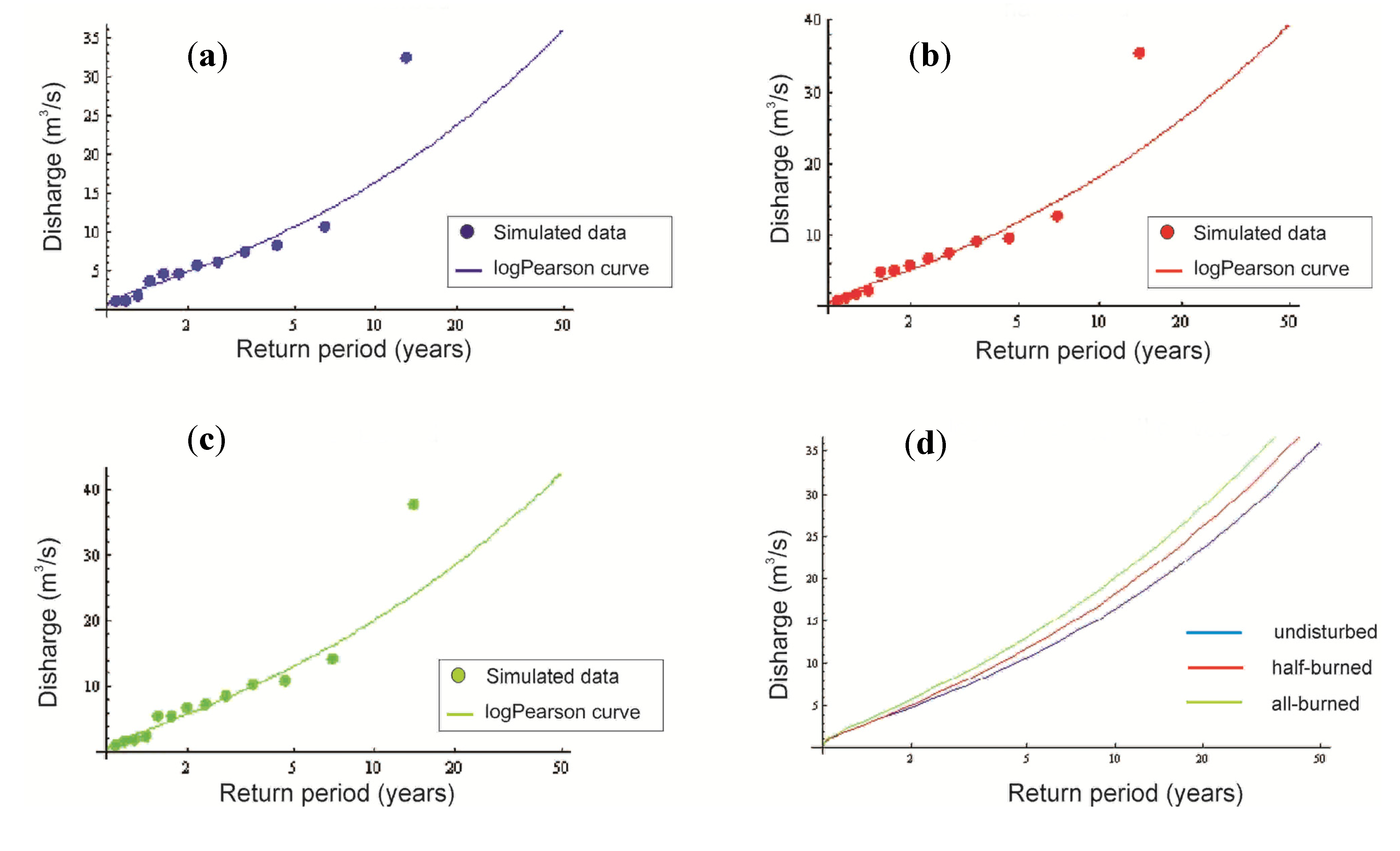
Furthermore, a flood frequency analysis of the annual maximum flood series for the Germasogeia watershed was performed to demonstrate the difference between the three scenarios, although it should not be used for large return periods since only 12 years of data exist. The log-Pearson Type III distribution was employed for the frequency analysis of the peak flows. Specifically, the well known formula was used:

log Q_p = y + K(p, γ) · S_y

(4)

where Q_p is the peak flow corresponding to frequency p. The measured values Q_i of the peak flows are transformed into their logarithms: y_i = Log(Q_i) and y is the mean value of the y_i’s. K(p,γ) is the frequency factor as a function of p and γ, where γ is the skew of this y-sample. Similarly S_y is the y-sample standard deviation. The expression for K(p,γ) is given in [20] and, for the needs of the present analysis, it was computed analytically instead of using tabled values.

Τhe logPearson type III was chosen based on the satisfactory fit shοwn in Figure 8a–c. Alternative distributions were considered with the help of Hydrognomon [21] free software for hydrological time series analysis. According to optical estimations and to the respective Kolmogorov-Smirnov test, four distributions stood out, without any appreciable differences among them. The results are given in the Table 5. Figure 8d shows the corresponding continuous distribution curves for the three different conditions, namely undisturbed, half-burned and burned forest, with discharge and return periods as coordinates. Thus, the comparative change in hydrological regime becomes clearer. It is also evident that the impact of forest cover change is larger on the peak flows of a large return period.

Figure 8. Fit of the log-Pearson Type III distribution to the three scenarios. (a) undisturbed; (b) half-burned; (c) all-burned; (d) logPearson type II curves.

Figure 8. Fit of the log-Pearson Type III distribution to the three scenarios. (a) undisturbed; (b) half-burned; (c) all-burned; (d) logPearson type II curves.

Table 5. Results of Kolmogorov-Smirnov test form Hydrognomon and for the undisturbed forest case. Similar results are obtained for the half-burnt and totally burnt cases.

Distribution	Attained a	DMax
LogNormal	99.66%	0.095
Galton	98.98%	0.106
LogPearson III	99.09%	0.104
GEV-Max	98.10%	0.113

Table 5. Results of Kolmogorov-Smirnov test form Hydrognomon and for the undisturbed forest case. Similar results are obtained for the half-burnt and totally burnt cases.

Distribution	Attained a	DMax
LogNormal	99.66%	0.095
Galton	98.98%	0.106
LogPearson III	99.09%	0.104
GEV-Max	98.10%	0.113

5. Conclusions

A compound tool was developed that couples the UBCWM to the MapInfo GIS. This tool combines the reliability and multiplicity of parameters of UBCWM with the data management and mapping capabilities of the GIS. The Germasogeia watershed in Cyprus was used as a case study for our tool. UBCWM requires multiple input parameters. Manual input of these input parameters for each of the 2419 cells in the Germasogeia watershed would be time consuming, tedious, and problematic. This study develops WM, an interface between MapInfo and UBCWM to derive, analyze, and visualize the required model parameters and simulated results from the databases of soil, topography and land cover. The interface consists of parameter generator, input file processor, model executor, output visualizer, statistical analyzer, and land use change simulator.

Application of the interface to the study of the watershed indicates that it is user friendly, robust, and significantly improves the efficiency of the modeling process. With the interface, land cover change scenarios can be readily explored in the model to help resource planners and decision makers develop watershed management plans.

Daily-recorded streamflow used for UBCWM validation indicated that the model is capable of reproducing the observed streamflow with accuracy. UBCWM application in three different scenarios concerning land use changes showed that decrease of forest area leads to increased frequency of intense peak flows.

The combined software tool presented in this paper may find a more general use by participating in unsteady hydrological analyses in situations where the existing time series contain trends and/or inhomogeneities due to systematic or isolated changes within the watershed [22].