Improving Sediment Transport Prediction by Assimilating Satellite Images in a Tidal Bay Model of Hong Kong


Abstract
:1. Introduction
2. Materials and the Model
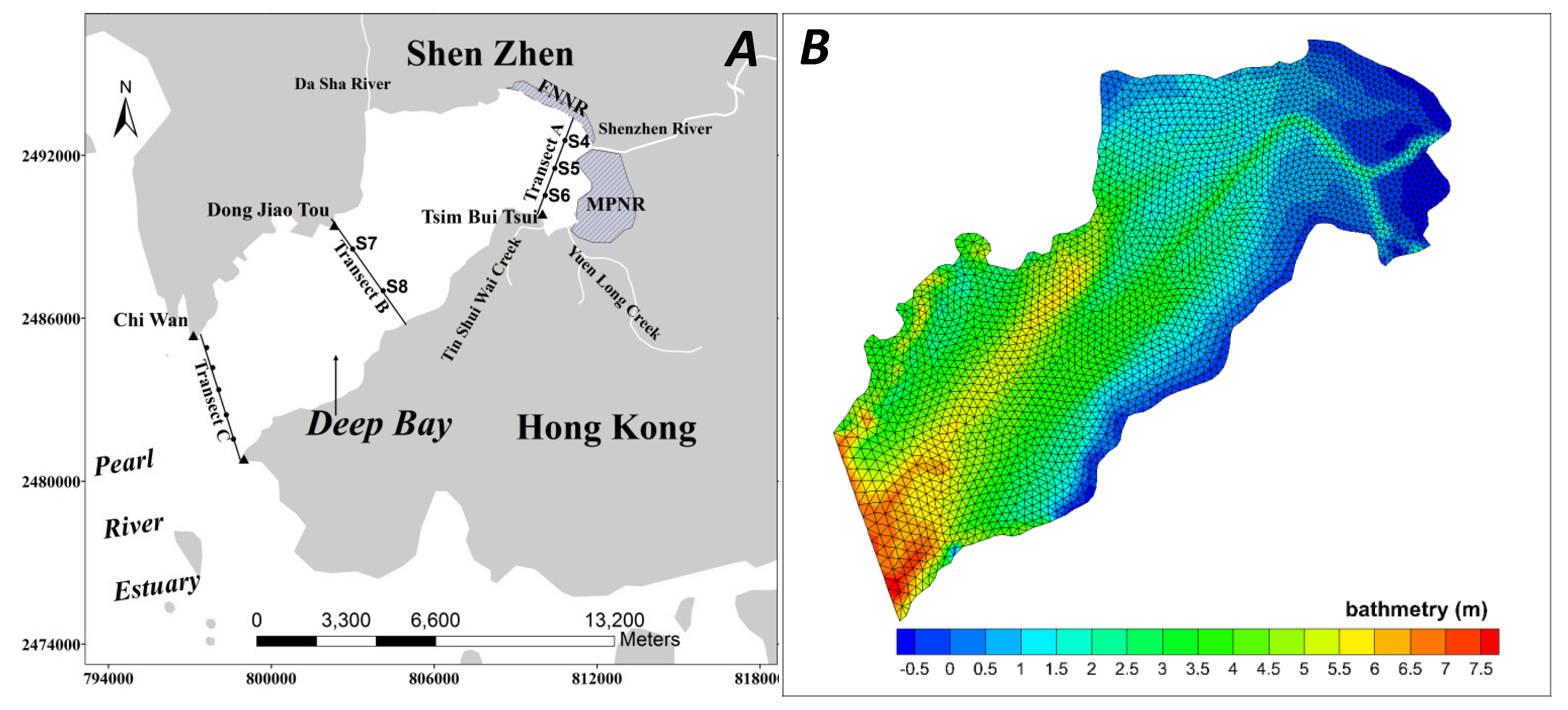
2.1. Study Area and In Situ Data

2.2. Model Description and Configuration

| Parameter | Shenzhen River | Dasha River | Yuen Long River | Tin Shui Wai River |
|---|---|---|---|---|
| V (m3/s) | 1.4 | 0.47 | 0.34 | 0.23 |
| C (mg/L) | 30 | 10 | 10 | 10 |
3. Methods
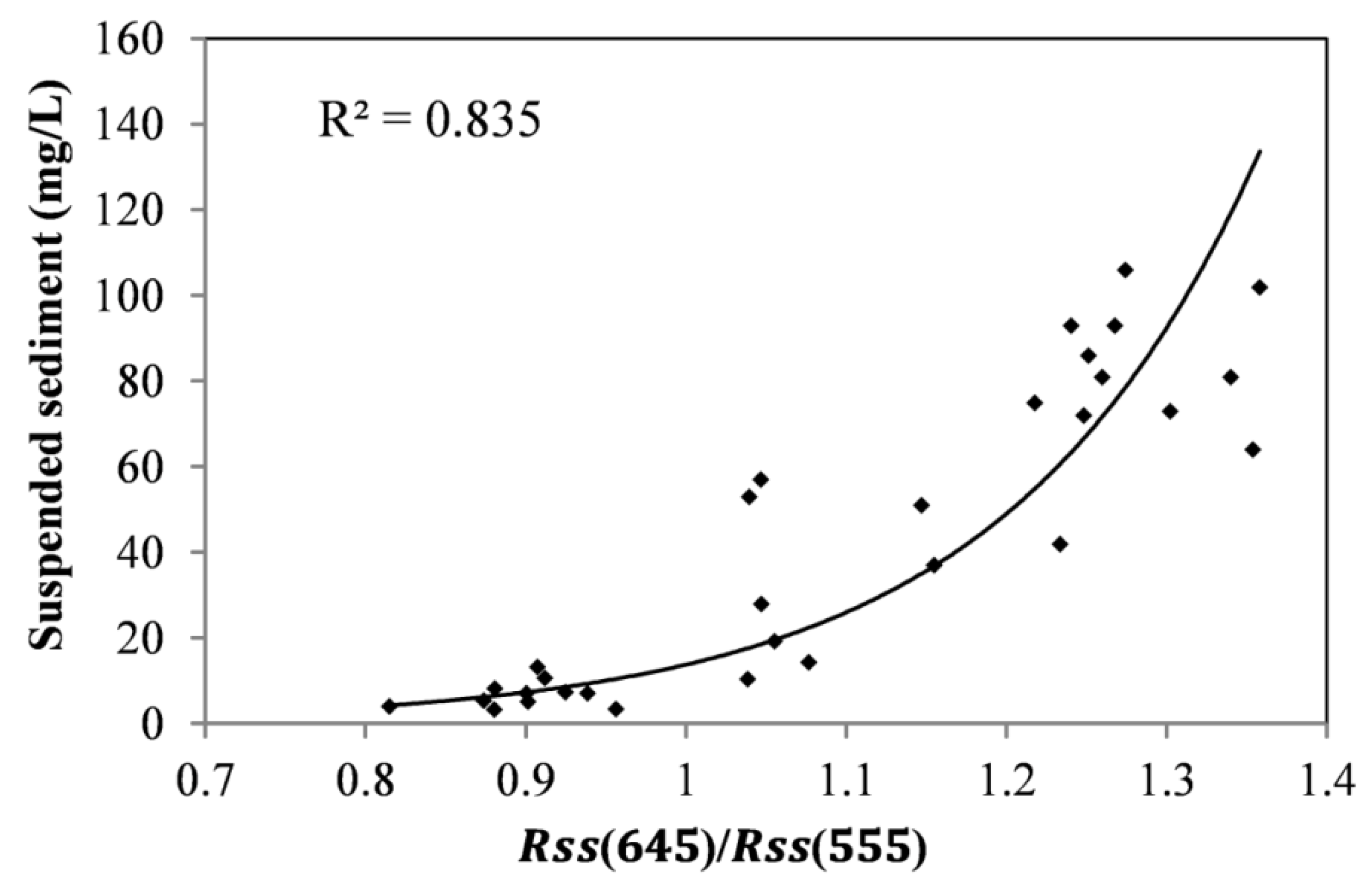
3.1. Satellite Sediment Information Retrieval

3.2. Assimilation Scheme


 ,
,  are the error variances of forecasted sediment concentration and remote sensing sediment concentration, with subscript k denoting the assimilation time.
  denotes the in situ measured sediment concentration at the i-th in situ site. N is the number of in situ measurement sites. The error variances of model forecast and remote sensing sediment concentration were calculated as 739.84 and 28.09, respectively.

 and
and  denote the sediment concentration from OI results and in situ measurement sites. N is the number of in situ measurements. The RMSE is also used to evaluate the model performance to forecast water level, salinity, current velocity and sediment concentration.
 4. Results and Discussion
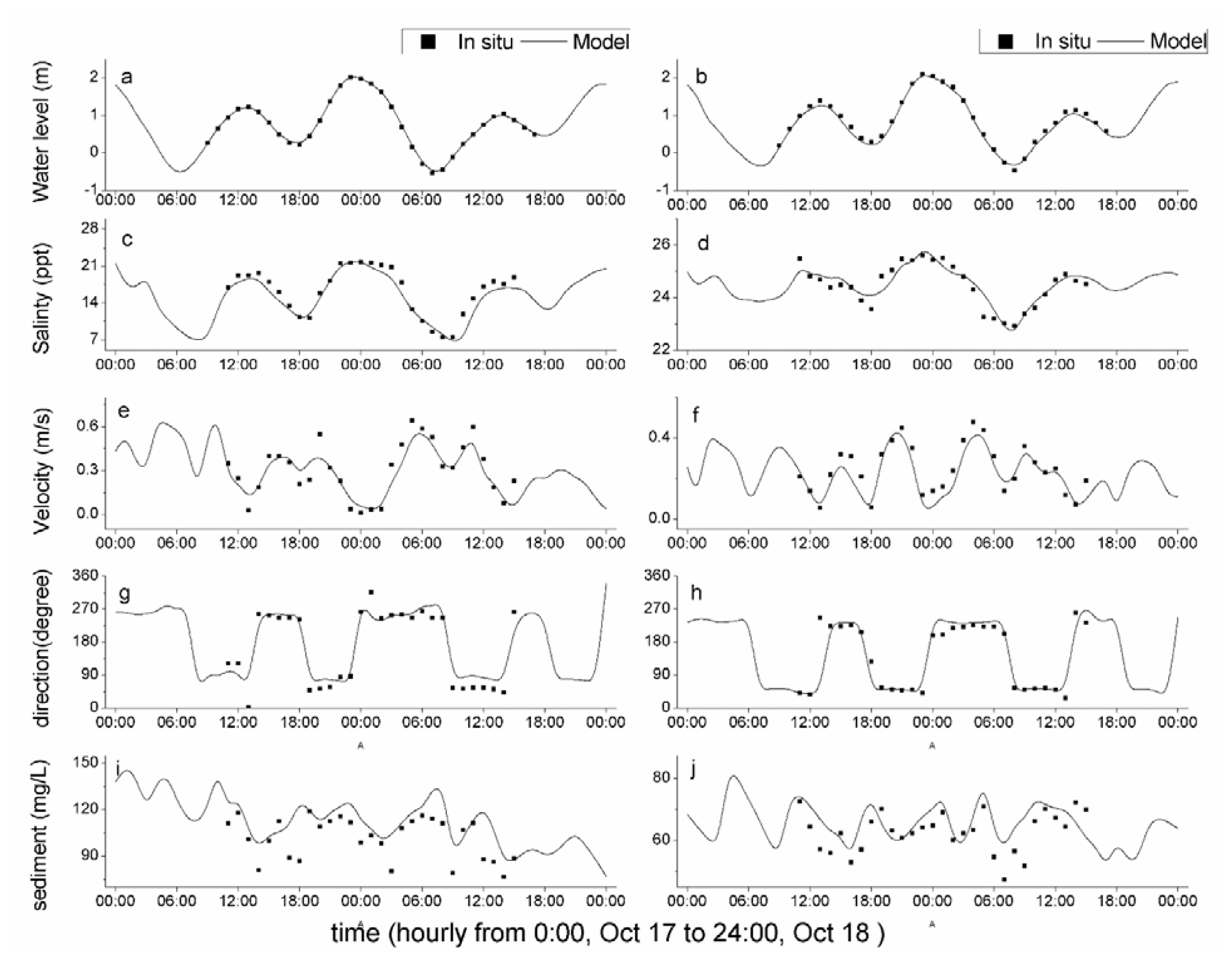
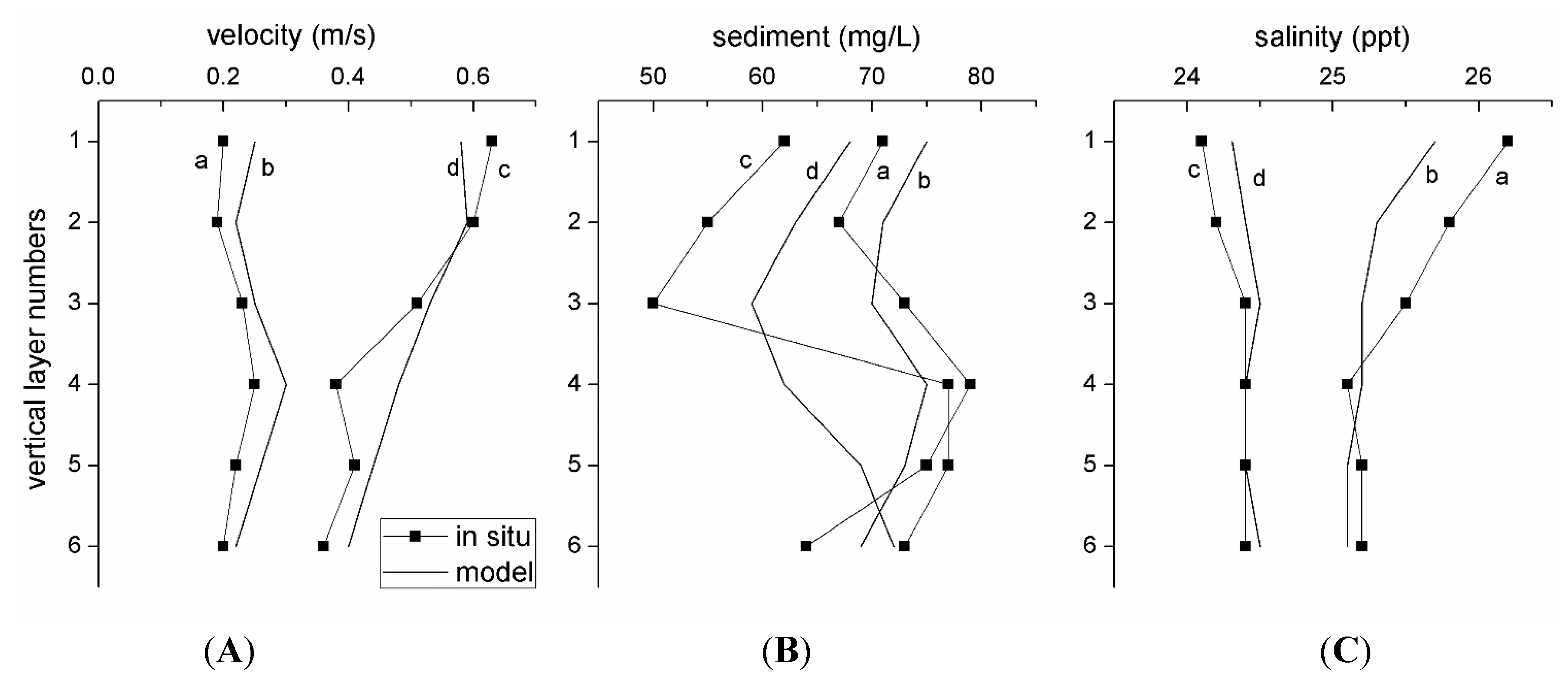
4.1. Model Calibration and Validation
| Parameters | Value |
|---|---|
| Bottom friction coefficient | 0.0024 |
| Sediment median diameter | 0.011 mm |
| Erosion constant | 1.2 × 10⁻⁵ kg/m2/s |
| Critical shear stress for erosion | 0.2 N/m2 |
| Critical shear stress for deposition | 0.08 N/m2 |
| Settling velocity | Ws = 0.014 × c1.3 m/s, c ≥ 60 mg/L
Ws = 5 × 10⁻⁵ m/s, c < 60 mg/L |


4.2. Assimilation Result Analysis
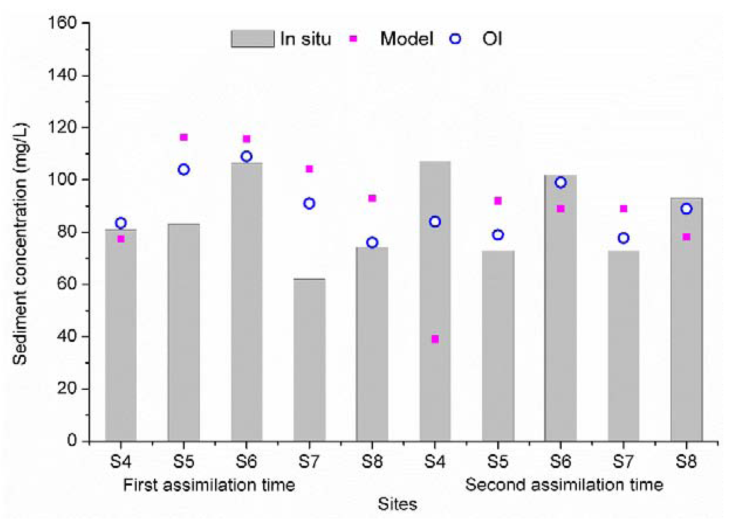
4.2.1. Sediment Correction at the Data Assimilation Time


| Assimilation time | Difference | Mean (mg/L) | Variance (mg/L) |
|---|---|---|---|
| AT1 | OI-RS | 2.5 | 21.16 |
| OI-Model | 7.8 | 492.84 | |
| AT2 | OI-RS | 1.4 | 8.41 |
| OI-Model | −10.6 | 979.69 |
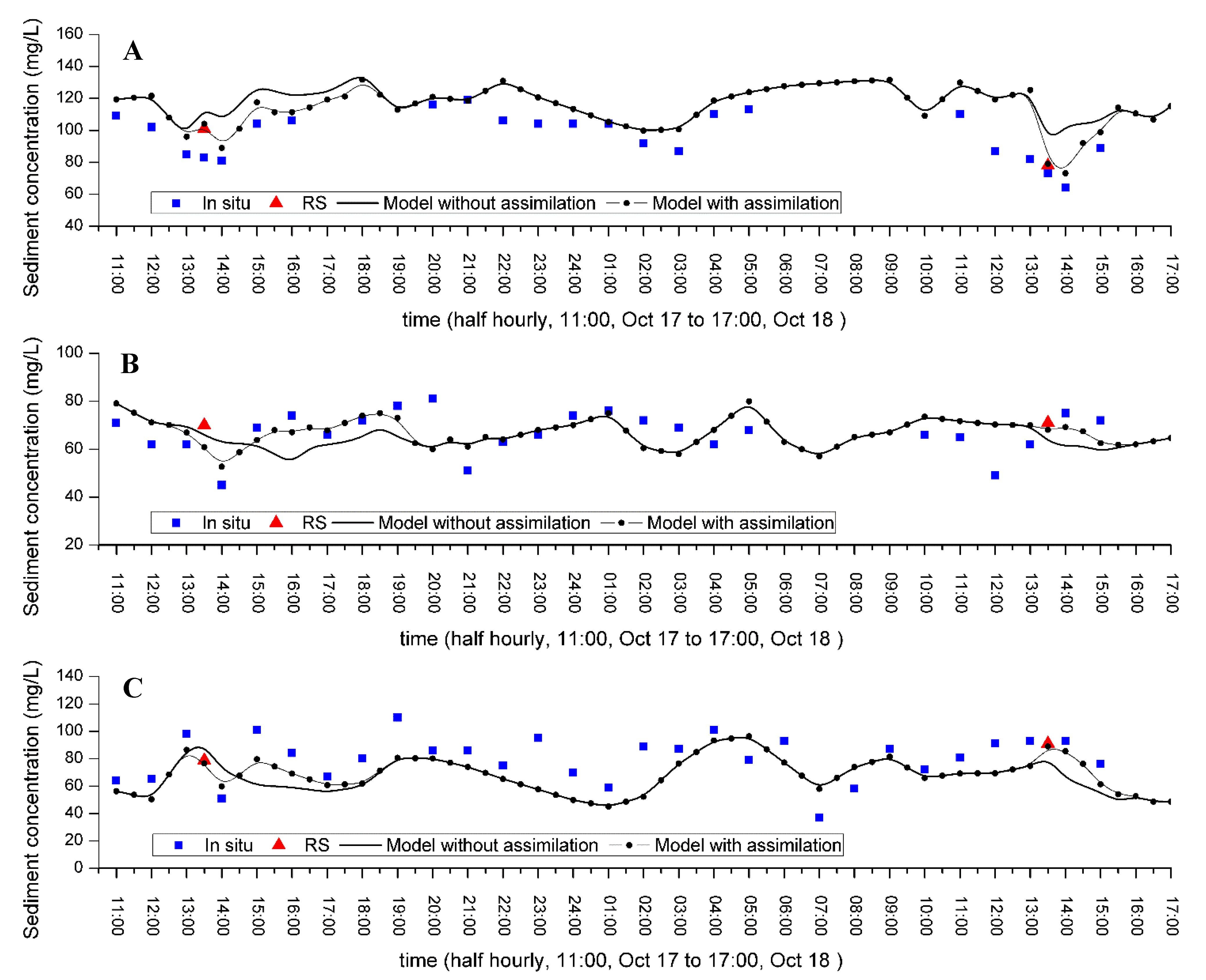
4.2.2. Temporal Effect of Data Assimilation

| Sites | Model without OI | Model with OI | Relative RMSE Reduction |
|---|---|---|---|
| surface sediment | |||
| S5 | 18.2 | 7.5 | 58.8% |
| S7 | 13 | 6.1 | 53.1% |
| S8 | 25.1 | 13.1 | 47.8% |
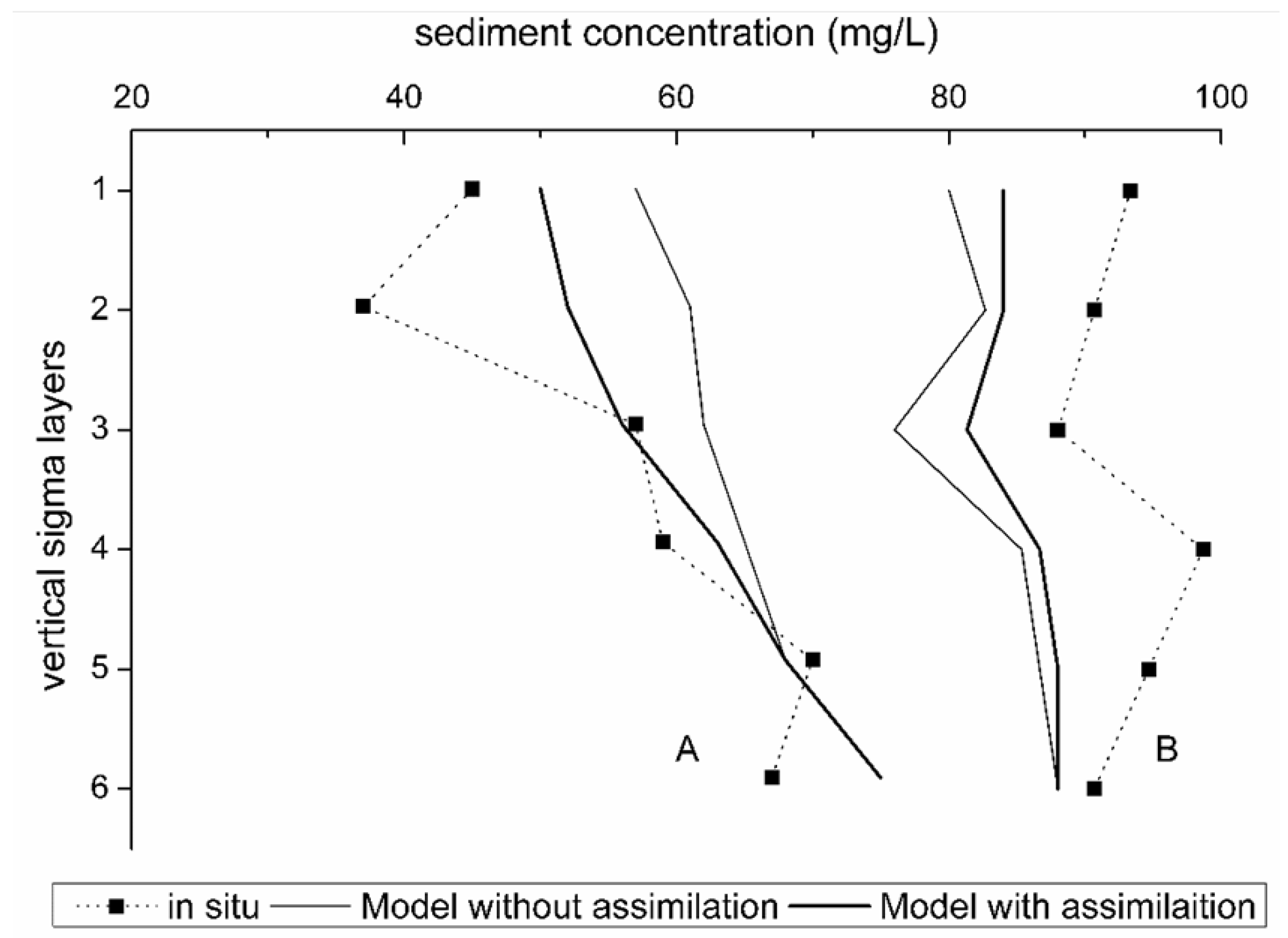
| depth-averaged sediment | |||
| S4 | 17.5 | 11.2 | 36.0% |
| S5 | 25.2 | 9.3 | 63.0% |
| S6 | 29.4 | 15.4 | 47.6% |
| S7 | 15.5 | 9.7 | 37.4% |
| S8 | 21.7 | 11.9 | 45.2% |

5. Conclusions and Outlook
Acknowledgments
Conflicts of Interest
References
- Onishi, Y.; Serne, J.; Arnold, E.; Cowan, C.; Thompson, F. Critical Review: Radionuclide Transport, Sediment Transport, Water Quality, Mathematical Modelling and Radionuclide Adsorption/desorption Mechanism; NUREG/CR-1322; Pacific Northwest Laboratory: Richland, DC, USA, 1981; p. 512. [Google Scholar]
- Smith, P.J.; Dance, S.L.; Nichols, N.K. A hybrid data assimilation scheme for model parameter estimation: Application to morphodynamic modelling. Comput. Fluids 2011, 46, 436–441. [Google Scholar] [CrossRef]
- Amoudry, L.O.; Souza, A.J. Deterministic coastal morphological and sediment transport modeling: A review and discussion. Rev. Geophys. 2011, 49. [Google Scholar] [CrossRef]
- Stroud, J.R.; Lesht, B.M.; Schwab, D.J.; Beletsky, D.; Stein, M.L. Assimilation of satellite images into a sediment transport model of Lake Michigan. Water Resour. Res. 2009, 45. [Google Scholar] [CrossRef]
- El Serafy, G.Y.H.; Mynett, A.E. Improving the operational forecasting system of the stratified flow in Osaka Bay using an ensemble Kalman filter-based steady state Kalman filter. Water Resour. Res. 2008, 44, W06416. [Google Scholar]
- Gregg, W. Assimilation of SeaWiFS ocean chlorophyll data into a three-dimensional global ocean model. J. Mar. Syst. 2008, 69, 205–225. [Google Scholar] [CrossRef]
- Pleskachevsky, A.; Gayer, G.; Horstmann, J.; Rosenthal, W. Synergy of satellite remote sensing and numerical modeling for monitoring of suspended particulate matter. Ocean Dyn. 2005, 55, 2–9. [Google Scholar] [CrossRef]
- Miller, R.L.; McKee, B.A. Using MODIS Terra 250 m imagery to map concentrations of total suspended matter in coastal waters. Remote Sens. Environ. 2004, 93, 259–266. [Google Scholar] [CrossRef]
- Kouts, T.; Sipelgas, L.; Savinits, N.; Raudsepp, U. Environmental monitoring of water quality in coastal sea area using remote sensing and modeling. Environ. Res. Eng. Manag. 2007, 1, 6. [Google Scholar]
- Chen, X.; Lu, J.; Cui, T.; Jiang, W.; Tian, L.; Chen, L.; Zhao, W. Coupling remote sensing retrieval with numerical simulation for SPM study—Taking Bohai Sea in China as a case. Int. J. Appl. Earth Obs. Geoinf. 2010, 12, S203–S211. [Google Scholar] [CrossRef]
- Yang, Z. Variational inverse parameter estimation in a cohesive sediment transport model: An adjoint approach. J. Geophys. Res. 2003, 108. [Google Scholar] [CrossRef]
- Margvelashvili, N.; Andrewartha, J.; Herzfeld, M.; Robson, B.J.; Brando, V.E. Satellite data assimilation and estimation of a 3D coastal sediment transport model using error-subspace emulators. Environ. Model. Softw. 2013, 40, 191–201. [Google Scholar] [CrossRef]
- EI Serafy, G.Y.; Eleveld, M.A.; Blaas, M.; Kessel, T.; Aguilar, S.G.; Woerd, H.J. Improving the description of the suspended particulate matter concentrations in the southern North Sea through assimilating remotely sensed data. Ocean Sci. J. 2011, 46, 179–204. [Google Scholar] [CrossRef]
- Lau, S.S.S.; Chu, L. The significance of sediment contamination in a coastal wetland, Hong Kong, China. Water Res. 2000, 34, 379–386. [Google Scholar] [CrossRef]
- Qin, H.P.; Ni, J.R.; Borthwick, A.G.L. Harmonized optimal postreclamation coastline for Deep Bay, China. J. Environ. Eng. 2002, 128, 10. [Google Scholar]
- Wang, Y.; Gu, J. Influence of temperature, salinity and pH on the growth of environmental Aeromonas and Vibrio species isolated from Mai Po and the Inner Deep Bay Nature Reserve Ramsar Site of Hong Kong. J. Basic Microbiol. 2005, 45, 83–93. [Google Scholar] [CrossRef]
- Zhang, J.; Cai, L.; Yuan, D.; Chen, M. Distribution and sources of polynuclear aromatic hydrocarbons in Mangrove surficial sediments of Deep Bay, China. Mar. Pollut. Bull. 2004, 49, 479–486. [Google Scholar] [CrossRef]
- Chen, C.; Huang, H.; Beardsley, R.C.; Liu, H.; Xu, Q.; Cowles, G. A finite volume numerical approach for coastal ocean circulation studies: Comparisons with finite difference models. J. Geophys. Res. 2007, 112. [Google Scholar] [CrossRef]
- Chen, C.; Liu, H.; Beardsley, R.C. An unstructured grid, finite-volume, three-dimensional, primitive equations ocean model: application to coastal ocean and estuaries. J. Atmos. Ocean. Technol. 2003, 20, 159–186. [Google Scholar] [CrossRef]
- Wong, S.H.; Li, Y.S. Hydrographic surveys and sedimentation in Deep Bay, Hong Kong. Environ. Geol. Water Sci. 1990, 15, 111–118. [Google Scholar] [CrossRef]
- MODIS Web. Available online: http://modis.gsfc.nasa.gov/ (accessed on 18 September 2013).
- Bernstein, L.S.; Adler-Golden, S.M.; Sundberg, R.L.; Levine, R.Y.; Perkins, T.C.; Berk, A.; Ratkowski, A.J.; Felde, G.; Hoke, M.L. A New Method for Atmospheric Correction and Aerosol Optical Property Retrieval for VIS-SWIR Multi- and Hyperspectral Imaging Sensors: QUAC (QUick Atmospheric Correction). In Proceedings of Geoscience and Remote Sensing Symposium, 2005, Seoul, Korea, 25–29 July 2005; pp. 3549–3552.
- Moses, W.J.; Gitelson, A.A.; Perk, R.L.; Gurlin, D.; Rundquist, D.C.; Leavitt, B.C.; Barrow, T.M.; Brakhage, P. Estimation of chlorophyll-a concentration in turbid productive waters using airborne hyperspectral data. Water Res. 2012, 46, 993–1004. [Google Scholar] [CrossRef]
- Dekker, A.G.; Vos, R.J.; Peters, S.W.M. Analytical algorithms for lake water TSM estimation for retrospective analyses of TM and SPOT sensor data. Int. J. Remote Sens. 2002, 23, 15–35. [Google Scholar] [CrossRef]
- Volpe, V.; Silvestri, S.; Marani, M. Remote sensing retrieval of suspended sediment concentration in shallow waters. Remote Sens. Environ. 2011, 115, 44–54. [Google Scholar] [CrossRef]
- Doxaran, D.; Froidfond, J-M.; Lavender, S.; Castaing, P. Spectral signature of highly turbid waters application with SPOT data to quantify suspended particulate matter concentrations. Remote Sens. Environ. 2002, 81, 149–161. [Google Scholar] [CrossRef]
- Han, Z.; Jin, Y.Q.; Yun, C.X. Suspended sediment concentrations in the Yangtze River estuary retrieved from the CMODIS data. Int. J. Remote Sens. 2006, 27, 4329–4336. [Google Scholar] [CrossRef]
- Feng, L.; Hu, C.; Chen, X.; Song, Q. Influence of the Three Gorges Dam on total suspended matters in the Yangtze Estuary and its adjacent coastal waters: Observations from MODIS. Remote Sens. Environ. 2014, 140, 779–788. [Google Scholar] [CrossRef]
- Hu, C.; Chen, Z.; Clayton, T.D.; Swarzenski, P.; Brock, J.C.; Muller-Karger, F.E. Assessment of estuarine water-quality indicators using MODIS medium-resolution bands: Initial results from Tampa Bay, FL. Remote Sens. Environ. 2004, 93, 423–441. [Google Scholar] [CrossRef]
- Wang, L.; Zhao, D.; Yang, J.; Chen, Y. Retrieval of total suspended matter from MODIS 250 m imagery in the Bohai Sea of China. J. Oceanogr. 2012, 68, 719–725. [Google Scholar] [CrossRef]
- Xi, H.; Zhang, Y. Total suspended matter observation in the Pearl River estuary from in situ and MERIS data. Environ. Monit. Assess. 2010, 177, 563–574. [Google Scholar]
- Liu, D.; Fu, D.; Xu, B.; Shen, C. Estimation of total suspended matter in the Zhujiang (Pearl) River estuary from Hyperion imagery. Chin. J. Oceanol. Limnol. 2012, 30, 16–21. [Google Scholar]
- Carton, J.A.; Chepurin, G.; Cao, X. A simple ocean data assimilation analysis of the global upper ocean 1950–95. Part I: Methodology. J. Phys. Oceanogr. 2000, 30, 294–309. [Google Scholar] [CrossRef]
- Fox, D.N.; Eague, W.J.T.; Barron, A.N. The modular ocean data assimilation system (MODAS). J. Atmos. Ocean. Technol. 2002, 19, 240–252. [Google Scholar] [CrossRef]
- Daley, R. Atmospheric Data Analysis; Cambridge University Press: Cambridge, UK, 1991; Volume 2. [Google Scholar]
- Larsen, J.; Høyer, J.L.; She, J. Validation of a hybrid optimal interpolation and Kalman filter scheme for sea surface temperature assimilation. J. Mar. Syst. 2007, 65, 122–133. [Google Scholar] [CrossRef]
- Høyer, J.L.; She, J. Optimal interpolation of sea surface temperature for the North Sea and Baltic Sea. J. Mar. Syst. 2007, 65, 176–189. [Google Scholar] [CrossRef]
- Mangiarotti, S.; Martinez, J.M.; Bonnet, M.P.; Buarque, D.C.; Filizola, N.; Mazzega, P. Discharge and suspended sediment flux estimated along the mainstream of the Amazon and the Madeira Rivers (from in situ and MODIS Satellite Data). Int. J. Appl. Earth Obs. Geoinf. 2013, 21, 341–355. [Google Scholar] [CrossRef] [Green Version]
- Xie, J.; Zhu, J. Ensemble optimal interpolation schemes for assimilating Argo profiles into a hybrid coordinate ocean model. Ocean Model. 2010, 33, 283–298. [Google Scholar] [CrossRef]
- Zhang, P.; Wai, O.W.H.; Chen, X.; Lu, J. Modeling sediment transport with current velocity assimilation in Deep Bay, Hong Kong, China. In Proceedings of 35th IAHR World Congress, Chengdu, China, 8–13 September 2013; pp. 1–6.
© 2014 by the authors; licensee MDPI, Basel, Switzerland. This article is an open access article distributed under the terms and conditions of the Creative Commons Attribution license (http://creativecommons.org/licenses/by/3.0/).
Share and Cite
Zhang, P.; Wai, O.W.H.; Chen, X.; Lu, J.; Tian, L. Improving Sediment Transport Prediction by Assimilating Satellite Images in a Tidal Bay Model of Hong Kong. Water 2014, 6, 642-660. https://doi.org/10.3390/w6030642
Zhang P, Wai OWH, Chen X, Lu J, Tian L. Improving Sediment Transport Prediction by Assimilating Satellite Images in a Tidal Bay Model of Hong Kong. Water. 2014; 6(3):642-660. https://doi.org/10.3390/w6030642
Chicago/Turabian StyleZhang, Peng, Onyx W.H. Wai, Xiaoling Chen, Jianzhong Lu, and Liqiao Tian. 2014. "Improving Sediment Transport Prediction by Assimilating Satellite Images in a Tidal Bay Model of Hong Kong" Water 6, no. 3: 642-660. https://doi.org/10.3390/w6030642