Detecting Emergence, Growth, and Senescence of Wetland Vegetation with Polarimetric Synthetic Aperture Radar (SAR) Data

Abstract

Wetlands provide ecosystem goods and services vitally important to humans. Land managers and policymakers working to conserve wetlands require regularly updated information on the statuses of wetlands across the landscape. However, wetlands are challenging to map remotely with high accuracy and consistency. We investigated the use of multitemporal polarimetric synthetic aperture radar (SAR) data acquired with Canada’s Radarsat-2 system to track within-season changes in wetland vegetation and surface water. We speculated, a priori, how temporal and morphological traits of different types of wetland vegetation should respond over a growing season with respect to four energy-scattering mechanisms. We used ground-based monitoring data and other ancillary information to assess the limits and consistency of the SAR data for tracking seasonal changes in wetlands. We found the traits of different types of vertical emergent wetland vegetation were detected well with the SAR data and corresponded with our anticipated backscatter responses. We also found using data from Landsat’s optical/infrared sensors in conjunction with SAR data helped remove confusion of wetland features with upland grasslands. These results suggest SAR data can provide useful monitoring information on the statuses of wetlands over time.

1. Introduction

Wetlands provide ecosystem goods and services vitally important to humans, including food, fiber, filtering of contaminants, sediment storage, flood control, wildlife habitat, recreation, aesthetic value, and others [1]. Many of these goods and services are realized at the local scale, but wetlands also provide important services at broader scales. Wetland-rich landscapes help regulate regional climate (e.g., [2]) and offer crucial habitat for intercontinental migratory species. Despite these benefits, wetlands have been drained extensively worldwide, mainly to provide acreage for cropland [3]. Shifts in climate regimes further threaten the persistence of wetlands [4].

U.S. and Canadian collaborators in the Terrestrial Wetland Global Change Research Network (TWGCRN [5]) are studying how key ecological conditions in wetland-upland landscapes change in relation to climate and land cover. One goal of this effort is to understand how intra- and interannual variations in precipitation and temperature relate to changes in landscape moisture availability, primary productivity, wetland habitat, and animal calling phenology and site occupancy over different temporal and spatial scales, and to assess how these conditions likely will change in the future. Resource managers and policymakers need such information to try to maintain the ecosystem services these landscapes provide in the face of global change (e.g., [6]).

TWGCRN partners measure ecological conditions across a set research nodes using complementary information from satellite- and ground-based sensors. The satellite measurements provide a broader geographic perspective of ecological conditions and are integral to establishing a landscape context for observations on the ground. However, wetlands have proven challenging to map remotely with high accuracy and consistency (e.g., see results in [7,8,9,10,11,12,13]) because the presence of water is highly dynamic and overstory vegetation can obscure wetlands viewed from above [14]. Also, the spatial extent of many wetlands is smaller than the resolvable capacity of most civilian satellite sensors, resulting in pixels where wetland components are eclipsed by upland components. Aerial sensors can provide data of high spatial resolution, and such data have been used for decades to map wetlands in the United States [15], but these data are expensive both to collect and interpret (typically highly labor intensive); thus, the repeat cycle for data acquisition and mapping is insufficient to study interactions between climate variables and wetland dynamics. Scientists in the TWGCRN continue to evaluate data from different sensors and approaches to map wetlands with sufficient reliability, consistency, and ease of use.

Research on wetlands by the remote sensing community often has focused on approaches that rely on information made available at no cost from passive optical/infrared satellite sensors, such as Thematic Mapper (TM) and Enhanced Thematic Mapper (ETM+) sensors on Landsat satellites and Moderate Resolution Imaging Spectroradiometers (MODIS) on Terra and Aqua satellites. However, these sensors detect energy reflected primarily from the top part of the vegetation canopy and operate within a part of the electromagnetic spectrum where wavelengths do not penetrate clouds, which can be common over wetland-rich landscapes.

Synthetic aperture radar (SAR) technology is attractive for mapping and monitoring wetlands remotely. These sensors provide their own energy source to detect features on the Earth’s surface and therefore are not limited to sunlight hours for collecting land-cover data. SAR systems operate at wavelengths in the microwave portion of the electromagnetic spectrum that can penetrate cloud cover and, to varying degrees, vegetation canopies. These systems are well suited to detect moisture in the landscape because water’s high dielectric constant increases the radar reflectivity of the land surface.

Many radar systems are designed to transmit and receive energy that is either horizontally (H) or vertically (V) polarized. Some satellite radar systems have offered “co-polarized” (transmitted and received as HH or VV) or “cross-polarized” (transmitted and received as HV or VH) data products that have proven useful for mapping water and monitoring flood events [7]. More advanced systems, such as Canada’s Radarsat-2 satellite, offer fully polarimetric data, that is, all four combinations of the transmission and reception planes (HH, VV, HV, and VH). These data provide a greater potential to harvest information about the structure and other characteristics of land-surface features by better capturing the ways in which the transmitted energy interacts with them. For example, four of the main types of energy backscatter are [16,17,18]: (1) no return to the radar system, which results from a specular (smooth) surface re-directing transmitted signals away from the radar source (e.g., calm water surface); (2) rough scattering, which is a single-bounce return from a non-smooth surface (e.g., choppy water surface or low-growing shrubs); (3) volume scattering, where radar signals are reflected by the surface of a canopy as well as by features beneath the surface and may represent multipath propagation (e.g., woodland); and (4) double-bounce scattering, which results from a right-angle reflector intersecting and redirecting a specular response back to the radar system (e.g., vertical emergent vegetation surrounded by exposed, calm water).

We investigated the use of multitemporal SAR data acquired with Canada’s Radarsat-2 satellite, a C-band system operating at a frequency of 5.405 GHz (5.6 cm wavelength), to assess if we could track changes in the extent of surface water and development of wetland vegetation over the course of a growing season, as well as distinguish differences between wetter and drier years. The types of radar derivatives we analyzed potentially could be produced operationally to monitor the statuses of wetlands, but we needed to evaluate whether we could interpret characteristics and processes of ecological interest with these data derivatives. For this assessment we selected the Tamarac National Wildlife Refuge, a TWGCRN research node offering a variety of wetland types and landscape settings and one of the research nodes less prone to cloud cover during the growing season. This latter characteristic allowed us to use data from optical/infrared sensors to augment our evaluation of the SAR data. We also took advantage of ground-based time-series data on wetland water levels collected by the TWGCRN, as well as several other types of ancillary information available for this node. We identified, a priori, temporal and morphological/foliar traits of wetland vegetation that we anticipated would affect characteristics of radar signal backscatter over the course of a growing season and, ultimately, provide information about the status of wetlands with respect to their hydrologic and biological cycles [19]. We used this collection of information to interpret whether spatiotemporal changes in the backscatter patterns of the SAR data over four growing seasons generally paralleled temporal patterns of weather (precipitation and air temperature) and water levels and spatial distributions of different types of wetland vegetation.

2. Methods

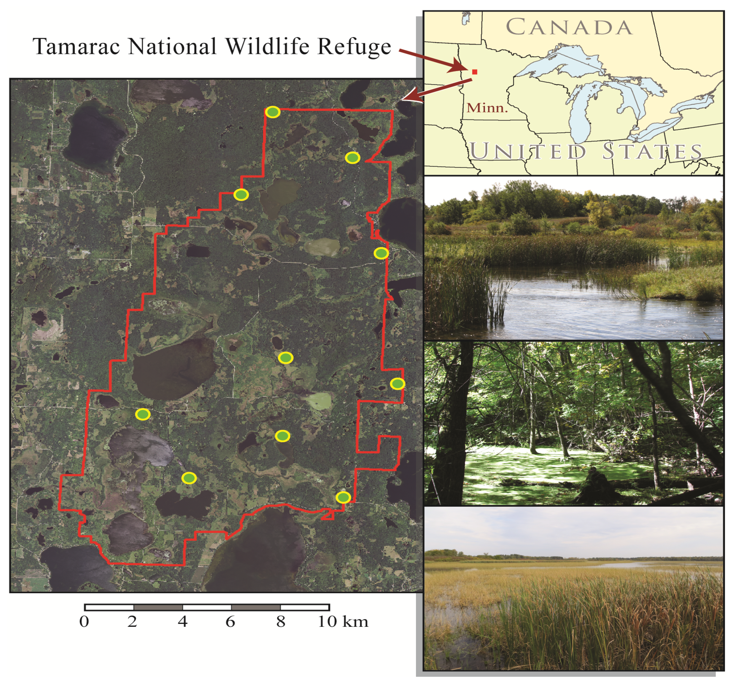
2.1. Study Area and Wetland Characteristics

The diversity of landscape settings in the Tamarac National Wildlife Refuge (NWR) in west-central Minnesota, USA, offered a basis to assess how consistently SAR data could detect wetland characteristics of interest for a variety of conditions. The area has a mix of vegetation types and species indicative of boreal forest, north-central hardwoods, and tallgrass prairie and includes a rich collection of lakes, temporary ponds, marshes, bogs, and swamps [20] (Figure 1) at various stages of development along continua [19] influenced by atmospheric and subsurface supplies of water. Tamarac NWR was established to support the interconnected wetlands and uplands needed by migratory birds and other wildlife, and monitoring statuses of wetlands is a key responsibility of Refuge staff.

Figure 1. Location and example photos of the wetland-rich landscape of the Tamarac National Wildlife Refuge in Minnesota, USA. Filled circles indicate distribution of wetlands monitored in situ.

Figure 1. Location and example photos of the wetland-rich landscape of the Tamarac National Wildlife Refuge in Minnesota, USA. Filled circles indicate distribution of wetlands monitored in situ.

Tamarac NWR has irregular plains of modest relief (30–90 m) averaging around 450 m above mean sea level. The area is snow-covered in winter, with snow and ice often lingering well into April and sometimes into May. Long-term (1981–2010) daily air temperatures over the growing season have averaged 12 °C for May, 17 °C for June, 20 °C for July, 19 °C for August, and 13 °C for September (30-year normal for Global Historical Climatology Network station USW00094967), after which the growing season winds to a close. Total monthly precipitation from May through September has averaged 76 mm, 109 mm, 89 mm, 80 mm, and 71 mm, respectively.

We focused our analysis on a set of wetland vegetation types for which we anticipated specific characteristics of SAR energy scattering over the growing season, based on the interplay between surface water and types of vertical emergent vegetation found in the Tamarac NWR (Table 1). Changes in water levels and growth of plants can alter relations between the scattering mechanisms as outlined in Table 1. For example, an increase in water level may cause an increase in double bounce if new vegetation is flooded or a decrease in double bounce if already-flooded vegetation becomes submerged. Similarly, plant growth may increase to the point of obscuring the water surface and decreasing double-bounce scattering while increasing volume scattering. It is these types of changes in the wetland conditions that we can try to monitor using SAR data. For the current study we focused our assessment on wetland types most likely to provide specular and/or double-bounce scattering detectable at C-band wavelengths. These included wetlands with no or very-low-growing herbaceous vegetation types and wetlands with medium to tall herbaceous vegetation types. We did not expect wetlands populated with low- to medium-height herbaceous vegetation types, such as sedge meadows, to be detected well with double-bounce scattering. In general, when water levels drop during the summer or for periods of prolonged drought, the low- to medium-height vegetation may no longer have standing water but will have wet, near-saturated soil. Although a wet soil surface will give a higher backscatter than a water surface, the vegetation generally is too substantial for significant penetration to the soil with C-band wavelengths and the backscatter will mostly be governed by the plants as volume or rough scattering. This backscatter intensity will be higher than for open water, but usually less than would occur for flooded vegetation with a significant double-bounce component. We also did not expect the C-band wavelengths to adequately penetrate the vegetation canopy in woody wetlands to provide information about underlying conditions [21], and researchers studying woody wetlands have had varying success characterizing seasonal changes in woody wetlands with C-band SAR data in (e.g., [22,23,24]).

Table 1. General types of wetland vegetation in the Tamarac National Wildlife Refuge and anticipated qualitative energy-scattering characteristics. Note: very-low height is <0.2 m; low height is 0.2–0.5 m; medium height is around 1 m; and tall height is approximate ≥2 m.

Targeted for current study	Height, structure, and temporal characteristics of wetland vegetation	Expected energy scattering *
Yes	Open water, with or without submerged aquatic vegetation.	Unbroken water surface should exhibit specular reflectance throughout the growing season.
Yes	Very-low growing floating-mat vegetation (e.g., water lilies, duckweed, and pondweed).	Vegetation cover has very low stature that conforms to the surface of the water. Scattering characteristics should be comparable to slightly roughened open water (likely not distinguishable from open water).
Yes	Medium height to tall annual vertical emergent vegetation (e.g., bulrush and wild rice).	Water surface is not vegetated at the start of the growing season, but is punctuated by stems as plants emerge. Stem and foliar development continue over the season. Specular reflectance at the beginning of the season shifts to double-bounce scattering after emergent plant structures gain height and biomass sufficient to deflect the radar signal from/to the water surface. Potential to distinguish between bulrush and wild rice communities with multi-year monitoring because bulrush begins each season in the same locations as the previous season(s) anchored by underwater rhizomes while wild rice starts from seed each year, with emergence within a waterbody dependent on how wind and water distributed the previous year’s seeds and/or how maturing plants were entrained as floating mats under windy conditions and rising water levels.
Yes	Tall vertical emergent vegetation with perennial vertical structures (e.g., cattails). New stems and leaves emerge annually, but senesced structures from previous seasons remain in place for multiple growth cycles.	Senesced emergent stems surrounded by exposed surface water should enable double-bounce scattering at the onset of the growing season. Double-bounce response could diminish as the new season’s stems emerge and accumulate biomass if the combined new and old biomass obscures the water’s surface.
No **	Low- to medium-height annual vertical emergent vegetation (e.g., sedge meadows).	Vegetation cover often is dense, obscuring much of the water’s surface and reducing the opportunity for double-bounce scattering. Rough-scattering response is likely, with occasional small areas of specular or double-bounce scatter where sufficient canopy openings occur.

Notes: * These description are based on the assumption that wetlands retain standing water throughout the season and that water levels do not rise so high as to drown the vertical emergents; ** We did not target monitoring of this type of wetland vegetation because the opportunity for double-bounce response at C-band wavelengths was too limited to expect to detect these wetlands.

Table 1. General types of wetland vegetation in the Tamarac National Wildlife Refuge and anticipated qualitative energy-scattering characteristics. Note: very-low height is <0.2 m; low height is 0.2–0.5 m; medium height is around 1 m; and tall height is approximate ≥2 m.

Targeted for current study	Height, structure, and temporal characteristics of wetland vegetation	Expected energy scattering *
Yes	Open water, with or without submerged aquatic vegetation.	Unbroken water surface should exhibit specular reflectance throughout the growing season.
Yes	Very-low growing floating-mat vegetation (e.g., water lilies, duckweed, and pondweed).	Vegetation cover has very low stature that conforms to the surface of the water. Scattering characteristics should be comparable to slightly roughened open water (likely not distinguishable from open water).
Yes	Medium height to tall annual vertical emergent vegetation (e.g., bulrush and wild rice).	Water surface is not vegetated at the start of the growing season, but is punctuated by stems as plants emerge. Stem and foliar development continue over the season. Specular reflectance at the beginning of the season shifts to double-bounce scattering after emergent plant structures gain height and biomass sufficient to deflect the radar signal from/to the water surface. Potential to distinguish between bulrush and wild rice communities with multi-year monitoring because bulrush begins each season in the same locations as the previous season(s) anchored by underwater rhizomes while wild rice starts from seed each year, with emergence within a waterbody dependent on how wind and water distributed the previous year’s seeds and/or how maturing plants were entrained as floating mats under windy conditions and rising water levels.
Yes	Tall vertical emergent vegetation with perennial vertical structures (e.g., cattails). New stems and leaves emerge annually, but senesced structures from previous seasons remain in place for multiple growth cycles.	Senesced emergent stems surrounded by exposed surface water should enable double-bounce scattering at the onset of the growing season. Double-bounce response could diminish as the new season’s stems emerge and accumulate biomass if the combined new and old biomass obscures the water’s surface.
No **	Low- to medium-height annual vertical emergent vegetation (e.g., sedge meadows).	Vegetation cover often is dense, obscuring much of the water’s surface and reducing the opportunity for double-bounce scattering. Rough-scattering response is likely, with occasional small areas of specular or double-bounce scatter where sufficient canopy openings occur.

Notes: * These description are based on the assumption that wetlands retain standing water throughout the season and that water levels do not rise so high as to drown the vertical emergents; ** We did not target monitoring of this type of wetland vegetation because the opportunity for double-bounce response at C-band wavelengths was too limited to expect to detect these wetlands.

2.2. SAR Data

We acquired multitemporal SAR data for 2009–2012 collected with Radarsat-2’s Fine Quad Polarization Beam mode (Table 2; [25]). This mode provides fully polarimetric imaging, with a nominal spatial resolution around 8 m (5.2 m range and 7.7 m azimuth) and an effective spatial resolution around 30 m after filtering for image speckle (noise). All acquisitions were right-looking, single-look complex data from descending orbits.

Table 2. Overpass dates for Radarsat-2 synthetic aperture radar (SAR) imagery. Data for 2009 were acquired with Fine Quad Beam 12 (FQ12) *; data for all other years were acquired with FQ2 *.

Year	1st overpass	2nd overpass	3rd overpass	4th overpass
2009	15 May **	2 July	26 July	12 September
2010	20 May	13 June **	31 July	24 August **
2011	15 May **	8 June **	26 July **	12 September **
2012	2 June	20 July **	13 August **	6 September

Notes: * FQ12 has a near incidence angle of 31.3° and a far incidence angle of 33.0°; FQ2 has a near incidence angle of 20.0° and a far incidence angle of 21.8°; ** Post-acquisition visual examination of SAR image revealed windy surface conditions present during the overpass; however, no local data were available on wind speeds.

Table 2. Overpass dates for Radarsat-2 synthetic aperture radar (SAR) imagery. Data for 2009 were acquired with Fine Quad Beam 12 (FQ12) *; data for all other years were acquired with FQ2 *.

Year	1st overpass	2nd overpass	3rd overpass	4th overpass
2009	15 May **	2 July	26 July	12 September
2010	20 May	13 June **	31 July	24 August **
2011	15 May **	8 June **	26 July **	12 September **
2012	2 June	20 July **	13 August **	6 September

Notes: * FQ12 has a near incidence angle of 31.3° and a far incidence angle of 33.0°; FQ2 has a near incidence angle of 20.0° and a far incidence angle of 21.8°; ** Post-acquisition visual examination of SAR image revealed windy surface conditions present during the overpass; however, no local data were available on wind speeds.

We produced two types of output with the SAR data from each overpass: a thematic binary map of open water and layers for each of three major types of energy scattering. We followed procedures described in White et al. [26] to map open water. These steps included: (1) selecting HV polarization if there was visual evidence of windy conditions in the Radarsat-2 image, or HH polarization if wind was not apparent; (2) applying a 5 × 5 high-pass filter to the HH or HV data to enhance edges and sharp features in the image; (3) applying a 3 × 3 low-pass filter to the HH or HV data to smooth image noise; (4) rescaling results from each filter (i.e., the “edge” results and the “smooth” results) to decibel range; (5) manually selecting thresholds that distinguished water from non-water features in the rescaled results; (6) merging information across results into a single binary map of open water; and (7) applying a 3 × 3 modal filter to further clean the map of open water.

We mapped types of energy scattering with the Freeman-Durden decomposition approach [17], which is well suited for identifying vertical emergent vegetation via the double bounce output channel. We used the PSFREDUR utility within the PCI Geomatica^© software package (version 10.3.2) to partition the total power of each image pixel of the fully polarimetric SAR data into contributions from double-bounce, volume, and rough surface scattering responses. We selected this approach based on previous evaluation of several decomposition approaches [27] and because the direct relation of output to major energy-scattering mechanisms made interpretive sense within the context of vegetation structure and phenology and other environmental characteristics related to climate and moisture availability.

2.3. Ancillary Data

We used data from several sources to interpret and, to the extent possible, validate the information content and consistency of the SAR-derived maps of open water and polarimetric decompositions. We compiled data on water levels monitored at hourly intervals in situ at the deepest location per wetland for a set of wetlands located throughout the Tamarac NWR (see Figure 1). These ten wetlands (note, only four were instrumented in 2009) were selected by TWGCRN investigators using an unbiased randomized block design based on whether wetlands were wood frog (Lithobates sylvaticus) habitat; the area of inference therefore includes all such wetlands (which typically are palustrine with emergent vegetation) in Tamarac NWR. These monitored wetlands are smaller in size than wetlands we expected to map with the SAR data and are highly sensitive to evapotranspiration. They may dry completely by the end of summer while moderate-sized to larger wetlands continue to hold water. In this way the monitored sites serve as a general indicator of relative changes in moisture status across the Tamarac NWR.

We acquired data on total precipitation and average air temperatures from the closest weather station (Detroit Lakes, Minnesota, Remote Automated Weather Station, identification NWSID 212201) for which daily data were available with little or no interruption in collection from 2009 to 2012 [28]. We had access to an unpublished, detailed digital vegetation map (minimum mapping unit 0.4 ha) developed for the Tamarac NWR by analysts at the USGS Upper Midwest Environmental Sciences Center from color-infrared aerial photographs acquired 25 September 2005 (scale 1:15,840). We also acquired a detailed digital map of wetlands (minimum mapping unit around 0.4–1.2 ha, depending on landscape setting [29]) classified from 1982 aerial photography as part of the U.S. Fish and Wildlife Service’s National Wetlands Inventory (NWI) project [15]. We obtained available high-resolution (1 m spatial resolution) color orthoimagery from overflights on 26 June 2009 and 9 July 2010 (two of our study years) and from 13 July 2005 (year of the unpublished vegetation map) through the U.S. Department of Agriculture’s National Agriculture Imagery Program [30,31]. Finally, we downloaded all available non-cloudy satellite data from Landsat-5 Thematic Mapper (TM) and Landsat-7 Enhanced Thematic Mapper (ETM+) sensors (30 m spatial resolution) for each growing season from 2009 to 2012 (Table 3; [32]). We were fortunate that these years were largely cloud-free over Tamarac NWR, as clouds were a pervasive problem in Landsat imagery for 2013, where the first clear growing-season overpass did not occur until 6 September.

Table 3. Overpass dates for Landsat sensor data for the scene defined by Path 29/Row 027.

Sensor	2009	Sensor	2010	Sensor	2011	Sensor	2012
ETM+	22 May	ETM+	25 May	TM	5 June	ETM+	14 May
TM	30 May	TM	18 June	ETM+	29 June	ETM+	1 July
TM	1 July	ETM+	28 July	ETM+	31 July	ETM+	2 August
TM	18 August	TM	5 August	TM	24 August	ETM+	18 August
ETM+	26 August	ETM+	29 August	TM	9 September	ETM+	26 August
TM	19 September					ETM+	3 September

Table 3. Overpass dates for Landsat sensor data for the scene defined by Path 29/Row 027.

Sensor	2009	Sensor	2010	Sensor	2011	Sensor	2012
ETM+	22 May	ETM+	25 May	TM	5 June	ETM+	14 May
TM	30 May	TM	18 June	ETM+	29 June	ETM+	1 July
TM	1 July	ETM+	28 July	ETM+	31 July	ETM+	2 August
TM	18 August	TM	5 August	TM	24 August	ETM+	18 August
ETM+	26 August	ETM+	29 August	TM	9 September	ETM+	26 August
TM	19 September					ETM+	3 September

2.4. Evaluation of SAR Data Derivatives

We used a combination of approaches for a multiscale assessment that capitalized on available field and remote data to learn: (1) if our expectations were met for within-season backscatter responses from different wetland vegetation types (per Table 1); (2) how consistently the same wetland features could be recognized from year to year; (3) the lower size limits for which these features could be mapped; (4) the types of landscape features associated with false detections; and (5) how well we could integrate information across SAR products to derive a seasonal summary of the status of wetlands in the Tamarac NWR.

We compared the SAR open water maps and polarimetric decomposition layers with orthoimagery from 2009 and 2010 and the Tamarac NWR land-cover map derived from 2005 air photos. We conducted an informal visual assessment of the types and sizes of wetland features we could distinguish from the SAR products. We looked for upland landscape features that had backscatter responses similar to those from wetland features to evaluate if there were parts of the growing season when the upland features were less likely to be confused with wetlands.

We tested the accuracy of two maps of open water by comparing orthoimagery acquired on 26 June 2009 with the SAR water map for 2 July 2009 and orthoimagery acquired on 9 July 2010 with the SAR water map for 31 July 2010. We used ArcMap software (ESRI^® ArcMap 10.0) to select 1000 point locations at random (“Create Random Points” utility) across the Tamarac NWR, specifying only that no two locations could be closer than 100 m apart. We then categorized each point location as water or non-water from the orthoimagery. We labeled a location as “water” if it had water with no vegetation, submerged aquatic vegetation, or floating mats of very-low growing vegetation, as we expected all these conditions to exhibit responses consistent with specular surfaces. We eliminated 20 point locations that were on land/water boundaries or along the edge of the SAR image extent, and assessed how many of the remaining 980 locations were identified correctly as water/non-water in the SAR water maps.

At a broader scale we generated time-series graphs to compare whether refuge-wide temporal changes in total area of open water mapped with SAR data corresponded with information from weather records and wetland hydrographs. We used monthly estimates of the Palmer Drought Severity Index [33] for the northwestern climate division of Minnesota (which contains the Tamarac NWR), downloaded from the National Oceanic and Atmospheric Administration [34], to inform our expectations for water in the landscape. This drought index is based on principles of the balance between moisture supply and evapotranspiration demand, and indicates the severity of a wet or dry spell.

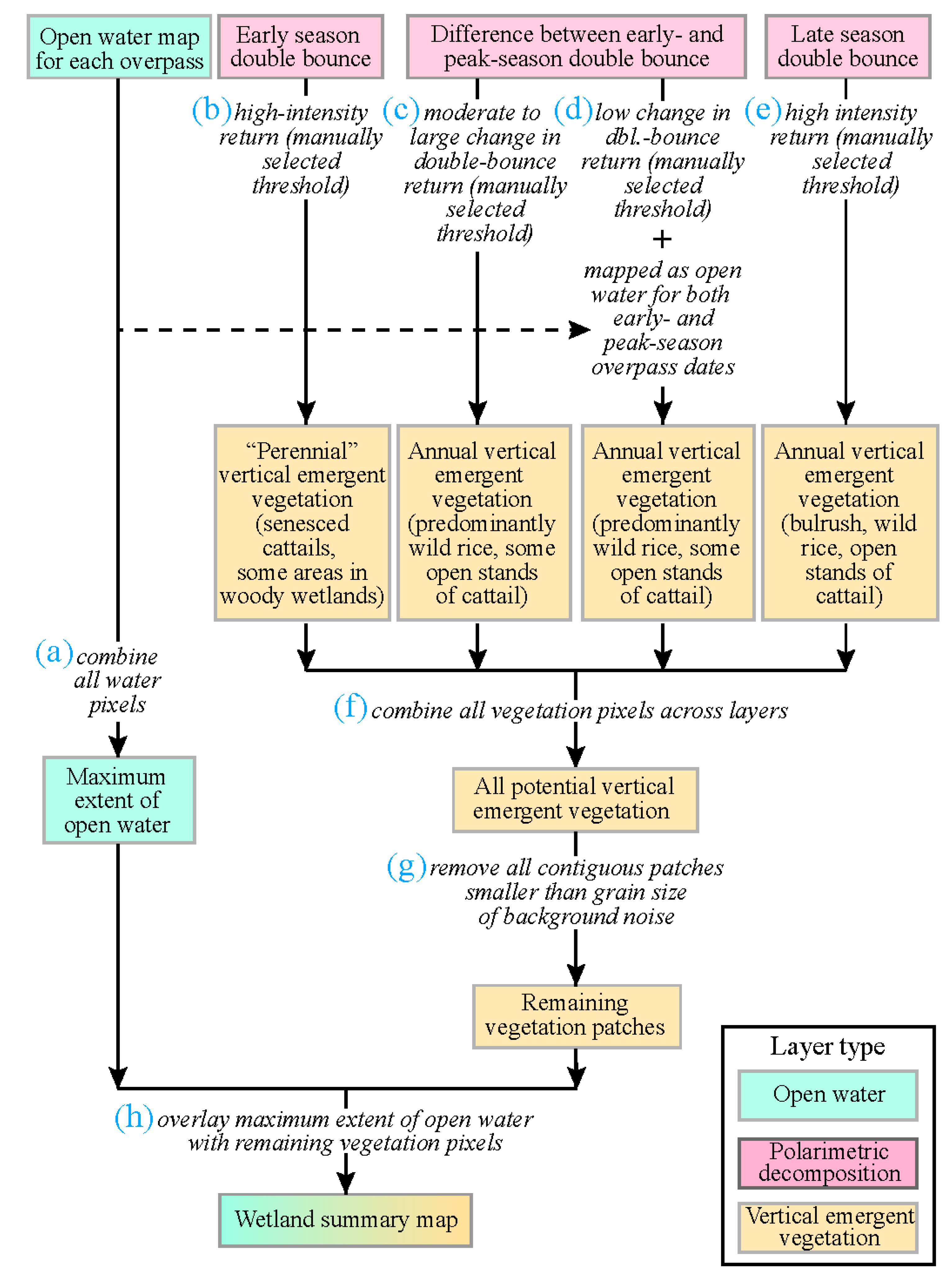
Developing Wetland Summaries

We used results from our evaluations of SAR derivative outputs to guide two general approaches to integrate information to compile a summary map of wetlands for each year. We relied only on SAR data derivatives for one approach (Figure 2) and complemented the SAR derivatives with data from optical/infrared sensors aboard Landsat satellites for the other approach (Figure 3). We could avoid relying on data dependent on daylight and cloud-free conditions with the first approach, which is important for regions often covered by clouds. The use of data from optical/infrared sensors, where feasible, enhances the ability to differentiate wetland features from uplands.

For both approaches we merged all pixels classified as water for any of the four overpasses per year to represent the maximum extent of water for the growing season (Figure 2a and Figure 3b). We treated the maximum water extent as background against which we overlaid pixels we identified as vertical emergent vegetation (Figure 2h and Figure 3i). This loosely reflected the process of open water becoming overtopped by vertical emergent canopies during a growing season. We examined the rough-scattering decomposition layers to identify windy overpass dates because wind is detrimental to the right-angle geometry needed for double-bounce response from non-woody plants in wetlands. We developed a set of criteria based on characteristics from Table 1 to identify pixels exhibiting the expected responses for different types of wetland vegetation, avoiding the use of imagery from windy dates, when we had the choice. We based all criteria on response thresholds we selected manually to extract: (1) high-intensity double-bounce scattering at the beginning of the growing season, decreasing over the remainder of the season (potential to capture senesced cattails [Typha angustifolia and T. latifolia] as well as less densely vegetated parts of bogs and swamps; Figure 2b and Figure 3c); (2) moderate to high increases in double-bounce response between early-season and peak-season overpasses (potential to capture bulrush [Schoenoplectus spp.], wild rice [Zizania aquatica and Z. palustris], and low-density areas of cattails; Figure 2c and Figure 3d); (3) high-intensity double-bounce scattering by late season (potential to capture fully developed biomass for bulrush, wild rice, and low-density areas of cattails, particularly if windy overpasses compromised results from the image-differencing of early- to peak-season changes in response; Figure 2e and Figure 3f); and (4) somewhat low increases in double-bounce response between early and peak season overpasses in locations also classified as water by the water-mapping algorithm (for HH or HV data) for both early- and peak-season dates (potential to capture bulrush, which would not yet have developed much biomass by peak season; Figure 2d and Figure 3e). We combined results from the (assumed) vegetation responses into an annual composite of vertical emergent vegetation (Figure 2f and Figure 3h).

Figure 2. Processing steps to generate summary maps of wetlands for each year using only SAR data.

Figure 2. Processing steps to generate summary maps of wetlands for each year using only SAR data.

Figure 3. Processing steps to generate summary maps of wetlands for each year using data from SAR and Landsat sensors.

Figure 3. Processing steps to generate summary maps of wetlands for each year using data from SAR and Landsat sensors.

Our two approaches for compiling summary maps diverged in how we handled potential errors of commission in mapping open water and wetland vegetation. Errors of commission can result from image speckle or from upland land-cover types exhibiting backscatter responses comparable with wetland features. Image speckle (noise) is inherent in radar data from sources in both the environment and the radar system equipment. The speckle has an observable spatial grain throughout the image. For the first approach (i.e., limited to SAR data) we calculated the areal extent for each patch of contiguous vegetation pixels meeting our criteria for double-bounce responses, then retained only those patches distinctly larger than the grain size of the image speckle (Figure 2g). For the second approach, where we supplemented SAR data with data from Landsat sensors, we used early-season information from the near-infrared part of the energy spectrum, a critical region for discriminating moisture [35]. We compared surface responses in the near-infrared band of Landsat TM and ETM+ data, calibrated to top-of-atmosphere reflectance (per [36,37]), with maps of wetlands as a preliminary step to proceeding with this approach. We found the spatial patterns of near-infrared responses in early-season Landsat sensor imagery were very similar to the geographic patterns of wetland types of interest we identified in the 2005 land-cover map for the Tamarac NWR (Figure 4). Later in the growing season, after the deciduous vegetation canopy was fully developed and occluded the ground surface, the near-infrared band became less informative about the moisture conditions of the substrate. We therefore used early-season imagery to stratify dry areas from potentially moist areas for mapping wetland vegetation. We also examined the correspondence between patterns of low near-infrared response with the distribution of wetlands available from the NWI. We found reasonable similarity between near-infrared patterns of response and the NWI distribution of wetlands, but the classification scheme used for the NWI did not permit us to differentiate our wetland types of interest from those of non-interest.

Figure 4. Comparison of early-season near-infrared (NIR) band reflectance (a) in 2011 with the distribution of water/wetlands from the 2005 land-cover map; (b) Low values of NIR reflectance (≤0.24 for this Landsat image date) coincided well with areas of water/wetlands; (c) including types of interest and those not targeted for the current study (refer to Table 1).

Figure 4. Comparison of early-season near-infrared (NIR) band reflectance (a) in 2011 with the distribution of water/wetlands from the 2005 land-cover map; (b) Low values of NIR reflectance (≤0.24 for this Landsat image date) coincided well with areas of water/wetlands; (c) including types of interest and those not targeted for the current study (refer to Table 1).

We used qualitative visual clues to manually selected a threshold level of reflectance for each Landsat date to stratify the imagery into areas that could have been moist (i.e., that exhibited low reflectance in the near-infrared band, where water absorbs energy) versus areas that likely were dry (i.e., that exhibited higher reflectance than the “moist” areas). We then appended our double-bounce criteria to require that pixels indicating potential wetland vegetation must be located within areas identified with Landsat data as “potentially moist” (Figure 3g).

As part of our second approach we also applied Landsat moist/dry landscape filters to reduce potential errors of commission in the maps of open water (Figure 3a). We selected the closest matching date of available Landsat TM or ETM+ imagery for each date of Radarsat-2 imagery to derive a separate mask per date to eliminate pixels classified as open water that were located in areas exhibiting near-infrared reflectance indicative of dry conditions.

The Landsat-7 ETM+ sensor’s faulty scan line corrector results in data gaps in the form of east-west image stripes that increase in width with increasing distance away from the central, north-to-south, swath of the image. Tamarac NWR is near the center of the swath track, which minimized data loss in cases where the most appropriate image was from a Landsat-7 overpass. Whenever we used data from the ETM+ sensor we filled data gaps with information from the closest subsequent or preceding date of cloud-free Landsat data. This solution is not ideal for characterizing environmental conditions with temporal dynamics finer than the overpass frequency, but we preferred this remedy to having no information for the data gaps.

3. Results

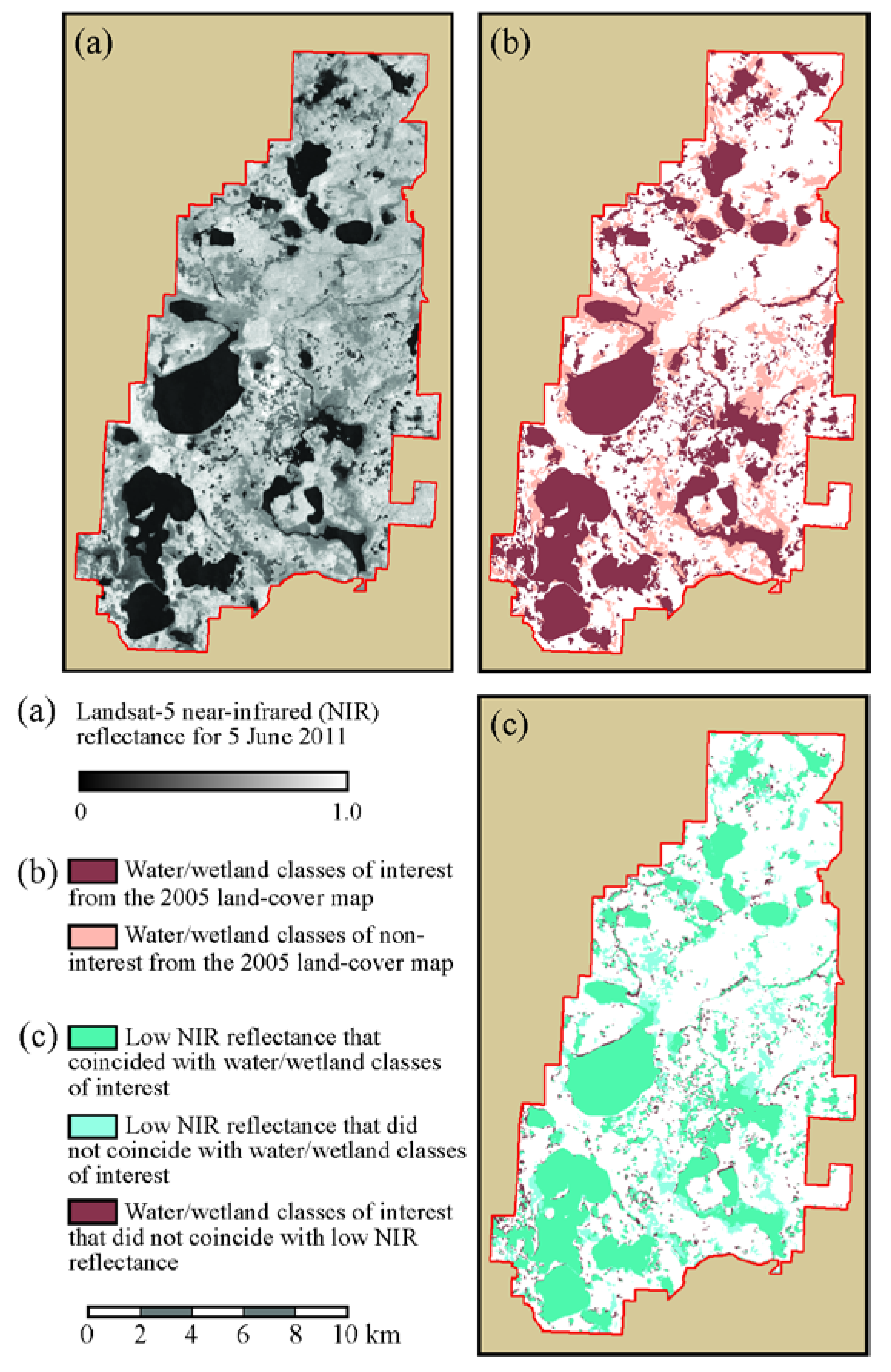
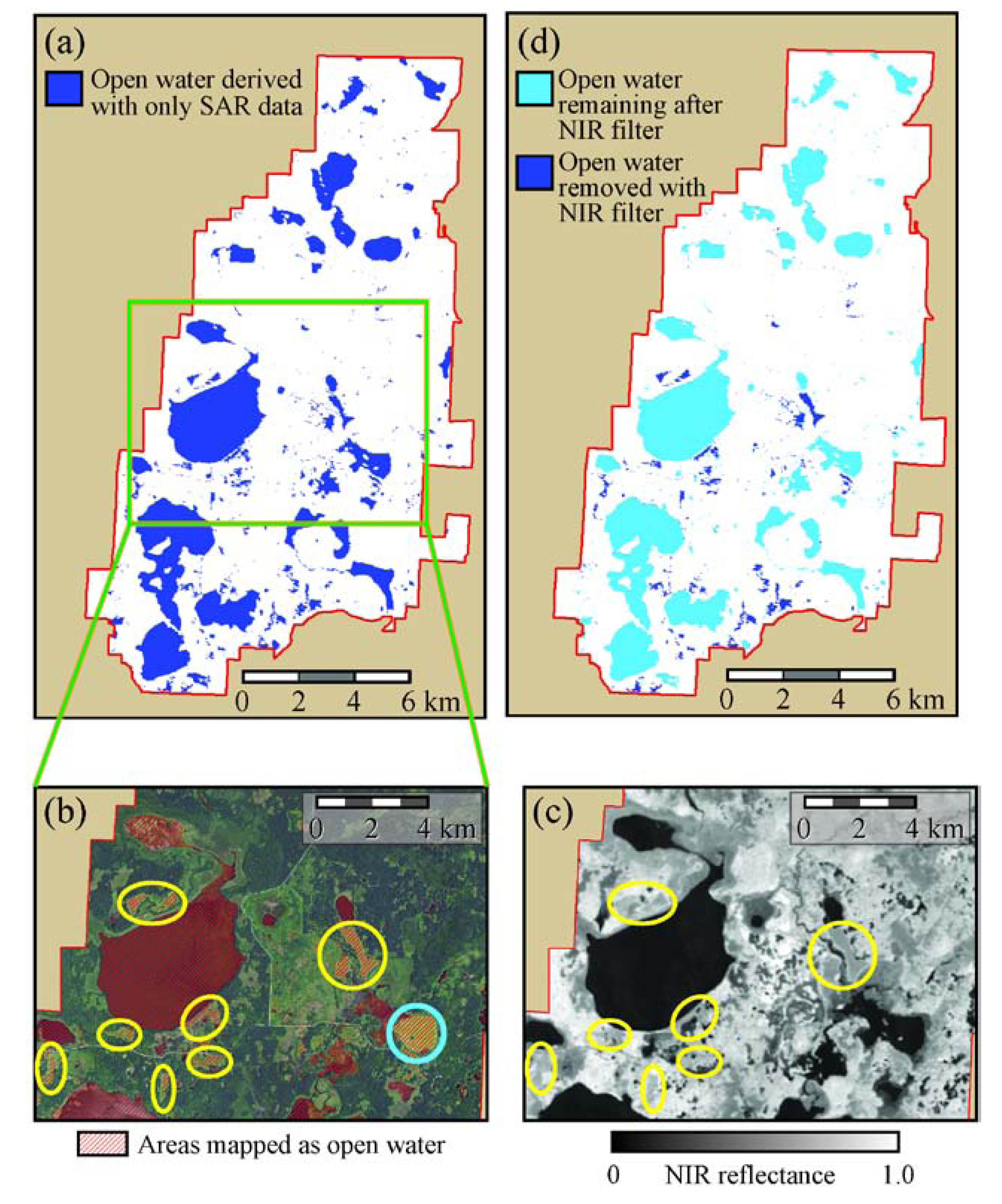
3.1. Evaluation of SAR Maps of Open Water

Rates of accuracy for mapping open water were 96%–98% for the 2009 date we tested and 97%–99% for the 2010 date, based on a 95% confidence interval for a normal approximation to a binomial distribution [38]. Main sources of error were grassy fields that routinely were classified as water, regardless of year or time of season (commission errors), inconsistent detection of waterbodies smaller than 100 m in the longest dimension (omission errors), inability to detect waterbodies beneath forest canopies (omission errors), and consequences inherited from a single threshold of energy backscatter selected to distinguish water from non-water (commission and omission errors). We addressed errors associated with confusing wetlands with upland grasslands by applying the near-infrared band filters we developed from best-match dates of Landsat data (Figure 5). The areal extent of this type of error of commission varied from date to date. We visually confirmed the near-infrared band filters were successful at removing grasslands routinely misinterpreted as open water from the water maps, but we had no good way to quantify the level of improvement.

Annual trajectories of total area mapped as water (after applying Landsat moist/dry filters) for each radar overpass were consistent with much, though not all, of the major temporal patterns in weather and water levels. In general, the SAR water derivatives showed the seasonal draw-down of water levels typical for this part of the country. The usual progression is for spring snowmelt and rainfall to fill wetlands early in the growing season when ground frost is present, deciduous vegetation is not fully leafed-out, and air temperatures still are relatively cool. Subsequent lengthening of diurnal photoperiod, warming of air temperatures, and development of the deciduous canopy all increase the demand on evapotranspiration, drawing down water supplies. Each of our study years offered its own variations on the combination of conditions that affect water levels. For example, annual accumulated precipitation was similar for 2011 and 2012 (although 2012 did tend to have larger precipitation events than did 2011), with neither year receiving much precipitation after mid-July (Figure 6a). A big difference between these years was that 2011 followed a very wet year and 2012 followed a dry year. In addition, air temperatures in 2012 were exceptionally high, resulting in drought conditions (Figure 6b), as evidenced by water drying in nearly all monitored wetlands that year (Figure 6c). The SAR maps showed similarities in extent of open water early in the season during 2011 and 2012 and captured the subsequent extraordinary drying of surface water in 2012 (Figure 6d).

Figure 5. Errors of commission in a map of open water derived from the SAR overpass of 8 June 2011. The water map generated with the initial algorithm we applied to HV data (a) included areas of grassy fields (encircled in yellow in (b)), a common outcome for nearly all dates of all years (the appearance of the area in (b) circled in blue, although similar to grassland, was turbid water). Landsat Thematic Mapper data for 5 June 2011 show that land-surface reflectance in the near-infrared (NIR) band was higher in the grassy areas than in areas of water/wetlands (c), enabling us to address this type of commission error with simple thresholding of the Landsat data (d).

Figure 5. Errors of commission in a map of open water derived from the SAR overpass of 8 June 2011. The water map generated with the initial algorithm we applied to HV data (a) included areas of grassy fields (encircled in yellow in (b)), a common outcome for nearly all dates of all years (the appearance of the area in (b) circled in blue, although similar to grassland, was turbid water). Landsat Thematic Mapper data for 5 June 2011 show that land-surface reflectance in the near-infrared (NIR) band was higher in the grassy areas than in areas of water/wetlands (c), enabling us to address this type of commission error with simple thresholding of the Landsat data (d).

Figure 6. Ground-based information on moisture versus extent of open water mapped with SAR data complemented with Landsat near-infrared data. Graphs of precipitation input (a) show interannual differences in delivery of water, both in individual events and in cumulative totals. The interplay between air temperature, moisture availability, and photoperiod affected the demand for evapotranspiration and resulted in varying drought status over time (b). Hydrographs for wetlands monitored in situ (c) corresponded with the changing conditions recorded in the precipitation record and with the estimated drought status (note: each colored line represents a different monitored wetland, and the same color is used for the same wetland across years). Total amount of water mapped with SAR data (d) captured some, but not all, of the general patterns of changing conditions in moisture availability. Note regarding (b): negative values of the Palmer Drought Index denote dry spells and positive values indicate wet spells. Values 0 to −0.5 = normal conditions; −0.5 to −1.0 = incipient drought; −1.0 to −2.0 = mild drought; −2.0 to −3.0 = moderate drought; −3.0 to −4.0 = severe drought; and greater than −4.0 = extreme drought. Similar adjectives are used for positive values of wet spells.

Figure 6. Ground-based information on moisture versus extent of open water mapped with SAR data complemented with Landsat near-infrared data. Graphs of precipitation input (a) show interannual differences in delivery of water, both in individual events and in cumulative totals. The interplay between air temperature, moisture availability, and photoperiod affected the demand for evapotranspiration and resulted in varying drought status over time (b). Hydrographs for wetlands monitored in situ (c) corresponded with the changing conditions recorded in the precipitation record and with the estimated drought status (note: each colored line represents a different monitored wetland, and the same color is used for the same wetland across years). Total amount of water mapped with SAR data (d) captured some, but not all, of the general patterns of changing conditions in moisture availability. Note regarding (b): negative values of the Palmer Drought Index denote dry spells and positive values indicate wet spells. Values 0 to −0.5 = normal conditions; −0.5 to −1.0 = incipient drought; −1.0 to −2.0 = mild drought; −2.0 to −3.0 = moderate drought; −3.0 to −4.0 = severe drought; and greater than −4.0 = extreme drought. Similar adjectives are used for positive values of wet spells.

Environmental conditions during the growing season in 2009 followed the classic cycle of spring filling of wetlands and subsequent decline in water levels over the course of summer, as shown in the wetland hydrographs (Figure 6c). Delivery of precipitation was fairly even throughout the growing season, but events usually were small (Figure 6a). We have no clear ground-based evidence from the hydrographs to explain the slight rise in the trajectory of the water extent from the second to the third SAR overpass in 2009 (Figure 6d), but the increase in mapped water was only 50 hectares and might be attributable to error/noise in the data rather that changing landscape conditions.

The temporal trajectory of water for 2010 was less straightforward to interpret from the SAR maps. In 2010 the snowpack melted soon after the start of March, which is early for the Tamarac NWR. There was little spring rainfall to fill wetlands (Figure 6a), nor was the previous year particularly wet. Several of the monitored wetlands began the season with lower water levels than in adjacent years (Figure 6c). Substantial rainfall began in mid-April, and July through August brought some very high precipitation events. Water levels in monitored wetlands were upward-trending over the season (Figure 6c), and from June onward, the cumulative precipitation was much higher in 2010 than in the other years (Figure 6a). The Palmer Drought Index estimated notably moist status at the beginning of the growing season in 2010 (i.e., there was enough moisture to meet the demand for evapotranspiration from the air temperatures), climbing to extraordinarily moist conditions by the end of the season (Figure 6b). The trajectory of surface water from the SAR maps reflected the drier start of the season and the delayed filling of the wetlands, but did not provide evidence for the substantial increase in moisture availability indicated by the weather data and wetland hydrographs. Some potential reasons the SAR water maps did not capture the wet conditions of the latter half of the 2010 growing season are: changes in water levels did not affect a wide enough swath along the margins of wetlands for the spatial resolving capacity of the sensor and/or for the algorithm used to map open water; the overstory vegetation canopy, once fully developed, obscured changes in the understory extent of surface water; very-low growing, floating-mat vegetation, such as duckweed and pondweed, so heavily obscured the underlying water by late summer that the surface became a rough target rather than a smooth target to the radar (the thresholding technique we used to map open water assumes smooth surface scattering); and/or the level of error introduced by subjective selection of thresholds when developing the water maps exceeded the amount of change in the extent of open water.

3.2. Evaluation of SAR Polarimetric Decomposition Layers

Annual time series of polarimetric decompositions developed with the Freeman-Durden approach revealed patterns of double-bounce scattering that aligned with our expectations for wetland vegetation morphology and phenological traits. We used the 2005 land-cover map, orthoimagery from 2005, 2009, and 2010, and our collective field experience at the Tamarac NWR to visually evaluate the decomposition output. Wetlands having no emergent vegetation or having very-low growing mats of vegetation remained free of double-bounce response over the season (Figure 7—example type 1). Areas that began the season with no double-bounce return, but developed a strong response by the peak or latter part of the season, were associated with stands of vertical emergent vegetation, typically wild rice, bulrush, and low-density zones of cattail. Bulrush was slower than wild rice to develop enough biomass for intense double-bounce return; hence, areas with bulrush were still being identified as open water (by the water algorithm) or as having low-intensity double-bounce backscatter as late as the peak of the growing season (Figure 7—example type 2). Wild rice, in comparison, had high-intensity backscatter by peak season (Figure 7—example type 3). Areas exhibiting a strong double-bounce return at the beginning of the season that showed a strong decrease in return by the end of the season were associated with dense stands of cattails or with woody wetlands such as tamarack bogs or alder swamps. Patterns of double-bounce scattering were spatially cohesive in cattail stands (Figure 7—example type 4), but diffuse in the woody wetlands. Low-density areas of cattails, such as along the advancing edge of a stand, had backscatter responses similar to wild rice and abutted an existing dense stands of cattails (Figure 7—example type 5).

Figure 7. Changes in intensity of double-bounce backscatter over the 2009 growing season. (a) Early-season overpass on 15 May; (b) peak-season overpass on 26 July; (c) late-season overpass on 12 September; and (d) difference between peak- and early-season intensity of double-bounce backscatter. Example types correspond with those referenced in Section 3.2.

Figure 7. Changes in intensity of double-bounce backscatter over the 2009 growing season. (a) Early-season overpass on 15 May; (b) peak-season overpass on 26 July; (c) late-season overpass on 12 September; and (d) difference between peak- and early-season intensity of double-bounce backscatter. Example types correspond with those referenced in Section 3.2.

We observed that early-season patterns of double-bounce backscatter generally included more noise from upland vegetation than in subsequent overpass dates. Prior to leaf-out, the trunks of trees rising from a bare understory provided double-bounce characteristics not unlike vertical emergent vegetation in wetlands. We also observed we could distinguish meaningful wetland vegetation features as small as 25–30 m in width in images representing double-bounce backscatter.

3.3. Integrating Information for Wetland Summaries

Developing wetland summary maps with only SAR-based data made it more difficult to remove noise from the data. We used a size threshold to remove all patches of potential vertical emergent vegetation that were at or smaller than the grain of the speckle pattern in the images. With this criterion we could retain features ≥5 ha in size, which represented only a few, large areas of wetland vegetation. Reducing the size threshold enabled us to retain more stands of vertical emergent vegetation, but also included many spurious patches not associated with wetlands.

We were much more successful in retaining wetland features in seasonal summary maps when we incorporated Landsat sensor data to help filter noise (Figure 5). Major patterns of water and wetland vegetation in our maps recurred across years, though there were interannual variations in details caused by actual changes in environmental conditions (areal expansion of vegetation communities and variations in water levels that affected vegetation emergence and development) as well as by artifacts from seasonal timing and wind conditions for Radarsat-2 overpasses (Figure 8). Nearly half (47%) of all pixels mapped as vertical emergent vegetation at some point during 2009–2012 were classified as vegetation in multiple years, and the patterns of the number of years a pixel was mapped as vegetation make interpretive sense, given variations in water levels (Figure 8). Most of the patterns for the number of times a pixel was mapped as water from 2009 to 2012 are related to them being mapped as vertical emergent vegetation in the other years. Exceptions are small areas in the southern part of the refuge that were mapped as water only once, but never as vertical emergent vegetation (see circled patches in Figure 8). These are grassy areas originally mapped with SAR data as open water in all years, but eliminated with the Landsat moisture threshold for years 2009–2011. In 2012 these areas had low reflectance in the near-infrared band at the beginning of the season (i.e., potentially were moist), which allowed them to be retained in the annual map as open water.

Seasonal summaries we generated with the steps diagrammed in Figure 3 showed distinctions among vegetation types and performed best when overpass dates were well distributed with respect to key periods of the growing season and there was little ambient wind to interfere with data collection, such as in 2009 (Figure 9). Early season, high-intensity double-bounce scattering (that subsequently decreased over the season, see Figure 7) occurred as fairly cohesive patches for stands of cattails, and as smaller, more diffuse patches in tamarack bogs and alder swamps. Areas showing moderate to high increase in double-bounce response between early- and peak-season periods often coincided with stands of wild rice. Areas having high-intensity returns later in the season, but that didn’t exhibit a high magnitude of change by peak season, tended to be bulrush, which has less biomass and dimensionality in structure than wild rice and probably did not develop sufficient biomass for double-bounce returns until late in the season. A few, very small, patches of bulrush in 2009 met our algorithm criterion for being mapped as open water for both early- and peak-season overpasses while also exhibiting low increases in double-bounce response in the polarimetric decomposition layers between those dates (Figure 2d and Figure 3e). In other years, we observed more patches meeting this particular combination of criteria, which may have resulted from interference from wind or to sparser distribution of vegetation stems per unit area from seasonal differences in environmental conditions.

Figure 8. Map showing the number of years for which a pixel was classified as vertical emergent vegetation or water.

Figure 8. Map showing the number of years for which a pixel was classified as vertical emergent vegetation or water.

Our wetland summary maps depicted patterns that generally corresponded visually with those from the 2005 land-cover map (e.g., Figure 9). There was fairly strong agreement in patterns associated with distributions of cattails and wild rice, as well as with the suggestion of patterns of woody wetlands where water levels and canopy openings permitted early-season double-bounce returns. Bulrush was not among cover types mapped in the 2005 land-cover classification, which is not surprising because the foliage does not have enough biomass to be distinguishable in color-infrared air photos, but informal field reconnaissance we conducted verified the presence of bulrush (e.g., Figure 9, photo 1), as well as other vegetation types (Figure 9, photos 2–4), for selected locations throughout the Tamarac NWR.

Figure 9. SAR seasonal summary map for 2009 (a) and the land-cover map developed from 2005 data (b). These maps show how the spatial distributions for different temporal characteristics of double-bounce backscatter compare with the distributions of wetland vegetation types from the land-cover map. Photo 1—bulrush; photo 2—large stand of cattails; photo 3—expanse of wild rice edged with narrow strips of cattails; photo 4—mix of wild rice and cattails established along a drainage.

Figure 9. SAR seasonal summary map for 2009 (a) and the land-cover map developed from 2005 data (b). These maps show how the spatial distributions for different temporal characteristics of double-bounce backscatter compare with the distributions of wetland vegetation types from the land-cover map. Photo 1—bulrush; photo 2—large stand of cattails; photo 3—expanse of wild rice edged with narrow strips of cattails; photo 4—mix of wild rice and cattails established along a drainage.

4. Discussion

We are interested in monitoring the dynamics of wetlands because they provide critical ecosystem services and because land-cover conversion and climate change threaten their persistence worldwide. Understanding how seasonal weather interacts with different hydrologic and land-cover settings to affect water dynamics is critical for discerning effects of climate change on wetlands. Wetlands naturally cycle through periods of flooding and drought that influence fluctuations and succession and that are important for maintaining ecological processes and functions [19]. Tracking longer-term changes in the vegetation characteristics and water levels of wetlands is informative about their successional status and ability to provide various ecosystem services, such as habitat or, as with the Tamarac NWR, an annual crop of wild rice (which is harvested by Native Americans).

We investigated the potential to use SAR data derivatives that could be produced semi-operationally for open water and types of energy-scattering to monitor extent of surface water and emergence, growth, and senescence of wetland vegetation. Interest in operational remote monitoring of wetlands is not unique to us. For example, the National Aeronautics and Space Administration (NASA) has funded a global-scale project to produce maps of inundation (i.e., fraction of land inundated with water) as a step towards operational monitoring of wetlands. These maps are being derived at a spatial resolution of approximately 25 km × 25 km with data from coarse resolution passive and active microwave sensors and optical/infrared sensors [39]. Our work targets finer spatial scales and informational detail relevant for resource managers charged with conserving wetlands to maintain ecological functioning, such as providing habitat for wetland-dependent species.

Use of SAR data to map water extent is not new [40,41], but recent availability of fully polarimetric SAR data is fostering new capabilities to monitor changes in wetland vegetation [8,42,43]. We incorporated data from Landsat’s optical/infrared sensors with SAR data to improve the accuracy of our wetland maps. Other researchers also have integrated data from optical/infrared and SAR systems to improve results of mapping wetlands (e.g., [44]), including the use of thresholds in the near-infrared band (e.g., [45]). We built upon this body of research by identifying specific annual traits of vegetation emergence, growth, and senescence that could be monitored with fully polarimetric SAR data. Outcomes from our work provide more specific information about tracking within-season development of wetland vegetation, as well as the potential to map vegetation types, to respond to information needs for those responsible for wetland conservation (e.g., [6]).

The method we implemented to map open water incorporated spatial resampling via a low-pass filter to reduce data noise and edge detection via a high-pass filter to identify land-water interfaces. Output from both steps required manual selection of a threshold of backscatter to distinguish water from non-water. We measured high rates of classification accuracy for water maps generated for two overpass dates. However, confusion of grasslands with open water and effects from over- or under-representing water because of the subjective selection of thresholds hindered our use of the maps for measuring changes in extent of open water over time. We filtered errors of commission with simple thresholding of Landsat data to exclude pixels routinely mapped as water that coincided with areas having levels of near-infrared reflectance indicative of upland or dry conditions. We lacked data appropriate to quantify levels of improvement these filters provided to our water maps, but confirmed visually with orthoimagery and topographic information that the resultant water maps no longer included obvious patches of upland grassland. We then compiled water information from the “filtered” maps to assess seasonal water dynamics at the scale of the Refuge. Our graph of extent of open water across the Tamarac NWR (Figure 6) showed a general annual pattern of greater amounts of open water at the beginning of the season, decreasing over the summer due to growth of emergent vegetation (water still present, but specular reflectance replaced by double-bounce response), and losses from evapotranspiration, runoff, and subsurface flow. Extent of open water mapped for 2012 was noticeably lower than for the other three years, which we would expect based on the Palmer Drought Index and wetland water levels that showed the majority of monitored sites went dry in 2012. Years 2010 and 2011 showed an upturn in open-water extent after mid-season (approximately after day 200 in Figure 6d), which corresponded with information in wetland hydrographs, but the minor uptick in open water mapped with SAR data for mid-2009 may have been due to mapping error, rather than changes in landscape conditions. Additional overpass dates would have helped us determine if this mapped increase in extent of open water was an artifact of mapping error or was supported across more dates of imagery.

We selected thresholds manually for the near-infrared data from Landsat sensors, which meant our results were susceptible to the same issues we faced with thresholds selected manually to map water with the SAR data. More objective methods exist for using Landsat data to map moisture (e.g., [11,46]), but results have been inconsistent or the methods are labor-intensive. We used only the near-infrared band from Landsat to stratify potentially moist areas because that part of the spectrum is highly informative about moisture in the landscape. However, other phenomena unrelated to moisture can exhibit similar responses in near-infrared wavelengths. Our results provided examples in the southern part of the Tamarac NWR, where grassy fields that had been burned just prior to the 2012 growing season had near-infrared reflectance responses similar to moist areas (Figure 8, circled areas). This type of problem can be minimized by incorporating additional Landsat data (e.g., from the thermal-infrared band) or ancillary data on burned areas (e.g., the MODIS Burned Area Product, available with near global coverage—although, this operational product has a spatial resolution of 1 km² [47]).

The years 2009–2012 provided extraordinary circumstances for studying moisture in wetlands of the Tamarac NWR. The growing season of 2009 had the greatest moisture surplus on record (dating back to 1895), as estimated by the Palmer Drought Index, and the growing season of 2012 was the 10th most droughty year by the same measure. This wide range of growing conditions was juxtaposed against different winter snowpacks and a very shallow depth-to-groundwater, resulting in a complexity of interactions reflected by our wetland hydrographs. All of this illustrates the importance of a monitoring system with complementary ground-based and satellite-borne sensors, as well as methods that are more automated and less subjective to produce results sufficiently consistent and accurate for operational monitoring. The science community continues to investigate more effective methods to automate mapping of surface water and flooding via temporal comparisons of SAR data to detect change (i.e., before and after flooding), use of optical data and land-cover classifications to identify areas more prone to flooding, and use of fine scale, high-precision elevation data to delineate terrain areas where flooding can occur [48,49,50].

We acquired SAR data from Radarsat-2’s Fine Quad Polarization Beam mode, but these fully polarimetric data were not required for mapping open water. Data sent and received in horizontal polarization are sufficient for mapping water under non-windy acquisition conditions, and dual polarization (HV) data can be used successfully when wind is a factor [51]. We observed no obvious impact to water maps we derived from data acquired during windy overpasses. Factors that did limit our ability to map water were SAR system wavelength and the method we used to reduce data speckle. Radarsat-2’s C-band wavelengths could not penetrate far enough into the closed woody canopies of the Tamarac NWR to provide information about water in the woodland understory. Longer wavelengths, such as the L-band system on ALOS-2, are better suited for such vegetation cover. The spatial averaging filter we used to reduce image speckle in the radar data substantially decreased the resolvable scale for water features; although we could detect waterbodies as small as 30 m in width, those we mapped with consistency across space and time were 100 m or larger in width. A near-term solution to resolve smaller waterbodies is to acquire data from beam modes of higher spatial resolution, such as Radarsat-2’s Spotlight mode, which has a nominal resolution around 1 m and, after spatial filtering, can resolve wetlands as small as 5 m in width (or likely around 10 m with consistency). The tradeoff for data of higher spatial resolution is a narrower swath width per overpass, increasing the number (and temporal separation) of side-lapping overpasses needed to cover an area of interest. The Spotlight mode also is not available as fully polarimetric data, limiting its use for mapping vegetation. Another option is to densify the time-series data stack sufficiently to implement temporal resampling, rather than spatial resampling, to reduce data speckle. This approach is becoming progressively more practical with the Radarsat Constellation Mission planned by the Canadian Government (designed to provide temporal coverage allowing for daily imaging over most of the Earth’s surface), the European and Asian SAR missions in place and planned, and an evolution in the business models for data distribution towards no- or low-cost availability of SAR data.

Fully polarimetric SAR data were necessary to decompose the scattering mechanisms we used to detect characteristics of vegetation emergence, growth, and senescence. We found the results showed potential to distinguish among vegetation types, which is encouraging for monitoring ecological dynamics. We used the Freeman-Durden approach to decompose the radar response signals into three main types of energy scattering, which we found straightforward to interpret with respect to our ecological knowledge of wetland features in the Tamarac NWR. There are other methods to characterize energy scattering with fully parametric data (some examples are listed in [8]), and these also may prove useful for applications like ours. Our results can be used to inform strategies for field campaigns to validate SAR-derived wetland maps, such as in considering resolvable area of features, vegetation morphology (complexity and robustness of vertical structures), stage of annual development, plant density per unit area, vegetation stand extent and shape, and water levels at the time of the SAR satellite overpass.

The vegetation features we could resolve consistently across years with the double-bounce response layers were fairly small (25–30 m in width) when we used Landsat data to filter errors of commission. At this resolution we were able to map the relatively narrow bands of vegetation often found along the edges of wetlands where water levels are shallower. We capitalized on temporal changes in vegetation structure and plant density to derive seasonal summary maps of reasonable spatial resolution for representing wetland habitat. We lacked data appropriate for a formal accuracy assessment or validation of the summary maps, given the available land-cover map was developed with imagery from 2005 and we are studying features that change annually in extent and density per unit area. We observed general agreement in patterns of wetland vegetation we mapped versus the 2005 land-cover map. Post-analysis informal reconnaissance of areas of disagreement revealed changes in vegetation cover since 2005 that supported the results we obtained with the SAR data (e.g., Figure 9).

Seasonal maps we generated without the benefit of Landsat data retained all errors of commission for open water (such as several sizeable grassland areas) and included only the largest (≥5 ha) contiguous patches of vertical emergent vegetation, as we spatially removed patches smaller than the grain size of the background noise pattern. These results might be useful for tracking changes in wetlands at broad regional to continental scales, but are less useful for scales at which land-management decisions are made. Given Landsat data are freely available and the archive dates back several decades, it is worthwhile to consider incorporating Landsat data into the wetland mapping procedures to help improve results. We experimented with two methods that could be used to generate Landsat moist/dry landscape filters for cloud-prone areas. For one method we searched the Landsat data archive [32] back through time to obtain an early-season overpass for the wettest possible year that provided cloud-free conditions to represent the maximum extent of landscape likely to include wetlands. We applied the filter we developed from this date to all SAR-derived water maps to reduce errors of commission. This approach would be feasible as long as current/future environmental conditions are not substantially wetter than those represented by historical wet conditions. For a second method we averaged the Landsat sensor data for the near-infrared band across early-season images from 2009 to 2012 to develop a single wet/dry filter from the results, which we then applied to all SAR-derived water maps. This method provided one, generally representative, filter across the years for which we had SAR data and could accommodate data gaps in the Landsat images either from the Landsat-7 scan line corrector or from clouds. Both methods appeared to perform reasonably well, certainly much better than not including a Landsat wet/dry filter.

Wind posed a major challenge for mapping vegetation. Wind during the early-season overpass compromised our ability to map cattails. If either the early-season or peak/late-season overpass was windy, it hindered results from image differencing that we needed to detect certain stands of wild rice and/or bulrush. Without results from the image differencing we only could distinguish stands exhibiting intense double-bounce returns during the latter half of the growing season, but had no way to extract the stands that had less-intense returns. For those, we required the magnitude of seasonal change in double-bounce response. Originally, we speculated that wild rice could be distinguished from bulrush based on spatial changes in annual seed establishment of wild rice (refer to Table 1). We remain uncertain if this is possible because the wetlands we knew contained wild rice at the beginning of our study years already were completely covered by the plants, and windy conditions in subsequent years compromised this aspect of our multiyear assessment. However, mapping results from 2009 suggest the timing of development (peak versus late season) and morphological differences in wild rice and bulrush are better ways to distinguish between these vegetation types (Figure 9).

The challenges imposed by wind-contaminated data and background data noise can be addressed with the same strategy: acquiring more dates of imagery per season. A denser time series will accommodate temporal filtering of noise (rather than spatial filtering), given that noise is spatially random, which ultimately will improve the spatial resolution of wetland features that can be mapped and the consistency with which they are detected with SAR data. Dense time series have not been feasible to assemble for most users of SAR data because of the difficulty and high costs associated with SAR data acquisition and processing. Availability and affordability of SAR data are evolving in ways that favor monitoring and multitemporal research. Some SAR specialists even have referred to the next decade as the Golden Age of SAR, given the number and variety of systems and constellations planned (including wavelengths from X- to L-band) and the shift in business models towards providing data at no or low cost to users. This bodes well for expanded opportunities to incorporate SAR systems with other satellite and ground-based sensors for operational, integrated monitoring of wetland landscapes.

5. Conclusions

We assessed the information value of SAR data derivatives representing open water and energy-scattering mechanisms for monitoring wetland characteristics we ultimately aim to relate to other types of responses we are measuring in wetland-upland landscapes as part of the TWGCRN. We used fully polarimetric data from Radarsat-2 and applied the Freeman-Durden approach to decompose microwave energy responses into three of the major types of scattering mechanisms we could anticipate and interpret in terms of cover types, plant morphology, and phenological traits of wetland-associated features. We learned we could extract features of wetland vegetation stands as small as 30 m in width with consistency across years. Our results suggest it is possible to distinguish among key vertical emergent vegetation types in the Tamarac NWR, including cattails, wild rice, and bulrush, when SAR overpass dates are well distributed with respect to key periods of the growing season and when there is little ambient wind to interfere with data collection. We also found we could reduce errors of mapping commission by incorporating early season data from Landsat optical/infrared sensors to complement the information content of the SAR data.

The growing-season time series of SAR data we acquired over four years clearly captured information about dynamics in selected types of wetlands, especially the interplay between water and vertical emergent vegetation. Time-series maps of open water we developed from HH and HV channel data were informative, but somewhat challenging to use for temporal tracking of changes in the extent of open water because the algorithm we employed included manual decisions about thresholds that could introduce errors into results. We refined our maps of open water by post-classification filtering with near-infrared band data from closest-match dates of Landsat overpasses.

We relied heavily on manual selection of thresholds throughout the steps we employed to educe wetland features. Our intent was to assess if the data derivatives captured the types of intra- and interannual dynamics we want to monitor in conjunction with other variables we are tracking in wetland-upland landscapes. We approached this assessment from a fairly straightforward, conceptual ecological basis. We determined we could interpret the information in the SAR data derivatives relative to other data we assembled regarding dynamics of weather, landscape moisture status, and land cover. This is encouraging for the goals of the TWGCRN, although we still face the challenge of translating a highly manual approach to one that is more sophisticated and automated.

The main problems we encountered with SAR data to map intra- and interannual changes in wetlands were related to reduced quality of information caused by wind during satellite overpasses and reduced spatial resolution of resolvable features caused by the spatial filtering we applied to remove data noise (speckle). Both types of problems can be addressed by increasing the density of the time-series stack for each growing season, a strategy that traditionally has not been feasible for most data users because SAR data are difficult and costly to acquire. Anticipated increases in availability and affordability of SAR data from a growing number of radar systems in orbit and shifts in data distribution policies that reduce or eliminate acquisition costs for users will make it much more feasible to monitor the influence of climate on wetland dynamics at scales appropriate for informing land-management decisions.

References

1. Millenium Ecosystem Assessment. Ecosystems and Human Well-Being: Wetlands and Water Synthesis; World Resources Institute: Washington, DC, USA, 2005. [Google Scholar]
2. Marshall, C.H.; Pielke, R.A., Sr.; Steyaert, L.T. Crop freezes and land-use change in Florida. Nature 2003, 426, 29–30. [Google Scholar] [CrossRef]
3. Baldassarre, G.A.; Bolen, E.G. Waterfowl Ecology and Management; John Wiley and Sons: New York, NY, USA, 1994. [Google Scholar]
4. Karl, T.R.; Melilo, J.M.; Peterson, T.C. Global Climate Change Impacts in the United States; Cambridge University Press: Cambridge, MA, USA, 2009. [Google Scholar]
5. Terrestrial Wetland Global Change Research Network. Available online: http://www.umesc.usgs.gov/twgcrn.html (accessed on 21 March 2014).
6. Eckles, S.D. Linking science, policy, and management to conserve wetlands in agricultural landscapes. Ecol. Appl. 2011, 21, S1–S2. [Google Scholar] [CrossRef]
7. Brisco, B.; Kapfer, M.; Hirose, T.; Tedford, B.; Liu, J. Evaluation of C-band polarization diversity and polarimetry for wetland mapping. Can. J. Remote Sens. 2011, 37, 82–92. [Google Scholar] [CrossRef]
8. Brisco, B.; Schmitt, A.; Murnaghan, K.; Kaya, S.; Roth, A. SAR polarimetric change detection for flooded vegetation. Int. J. Digit. Earth 2013, 6, 103–114. [Google Scholar] [CrossRef]
9. Brisco, B.; Short, N.; van der Sanden, J.; Landry, R.; Raymond, D. A semi-automated tool for surface water mapping with Radarsat-1. Can. J. Remote Sens. 2009, 35, 336–344. [Google Scholar] [CrossRef]
10. Corcoran, J.M.; Knight, J.F.; Gallant, A.L. Influence of multi-source and multi-temporal remotely sensed and ancillary data on the accuracy of random forest classification of wetlands in northern Minnesota. Remote Sens. 2013, 5, 3212–3238. [Google Scholar] [CrossRef]
11. Rover, J.; Wylie, B.K.; Ji, L. A self-trained classification technique for producing 30 m percent-water maps from Landsat data. Int. J. Remote Sens. 2010, 31, 2197–2203. [Google Scholar] [CrossRef]
12. Wickham, J.D.; Stehman, S.V.; Fry, J.A.; Smith, J.H.; Homer, C.G. Thematic accuracy of the NLCD 2001 land cover for the conterminous United States. Remote Sens. Environ. 2010, 114, 1286–1296. [Google Scholar] [CrossRef]
13. Wickham, J.D.; Stehman, S.V.; Gass, L.; Dewitz, J.; Fry, J.A.; Wade, T.G. Accuracy assessment of NLCD 2006 land cover and impervious surface. Remote Sens. Environ. 2013, 130, 294–304. [Google Scholar] [CrossRef]
14. Gallant, A.L. What you should know about land-cover data. J. Wildl. Manag. 2009, 73, 796–805. [Google Scholar] [CrossRef]
15. Wilen, B.O.; Bates, M.K. The US Fish and Wildlife Service’s National Wetlands Inventory project. Vegetatio 1995, 118, 153–169. [Google Scholar] [CrossRef]
16. Bourgeau-Chavez, L.L.; Smith, K.B.; Brunzell, S.M.; Kasischke, E.S.; Romanowicz, E.A.; Richardson, C.J. Remote monitoring of regional inundation patterns and hydroperiod in the Greater Everglades using synthetic aperture radar. Wetlands 2005, 1, 176–191. [Google Scholar]
17. Freeman, A.; Durden, S.L. A three-component scattering model for polarimetric SAR data. IEEE Trans. Geosci. Remote Sens. 1998, 36, 963–973. [Google Scholar] [CrossRef]
18. Wdowinski, S.; Sang-Wan, K.; Amelung, F.; Dixon, T.H.; Miralles-Wilhelm, F.; Sonenshein, R. Space-based detection of wetlands’ surface water level changes from L-band SAR interferometry. Remote Sens. Environ. 2008, 112, 681–696. [Google Scholar] [CrossRef]
19. Euliss, N.H., Jr.; LaBaugh, J.W.; Fredrickson, L.H.; Mushet, D.M.; Laubhan, M.K.; Swanson, G.A.; Winter, T.C.; Rosenberry, D.O.; Nelson, R.D. The wetland continuum: A conceptual framework for interpreting biological studies. Wetlands 2004, 24, 448–458. [Google Scholar] [CrossRef]
20. Butcher, R.D. America’s National Wildlife Refuges, 2nd ed.; Taylor Trade Publishing: Lanham, MD, USA, 2008; pp. 146–147. [Google Scholar]
21. Kasischke, E.S.; Melack, J.M.; Dobson, M.C. The use of imaging radars for ecological applications—A review. Remote Sens. Environ. 1997, 59, 141–156. [Google Scholar] [CrossRef]
22. Li, J.; Chen, W. A rule-based method for mapping Canada’s wetlands using optical, radar and DEM data. Int. J. Remote Sens. 2005, 26, 5051–5069. [Google Scholar] [CrossRef]
23. Lang, M.W.; Kasischke, E.S.; Prince, S.D.; Pittman, K.W. Assessment of C-band synthetic aperture radar data for mapping and monitoring Coastal Plain forested wetlands in the Mid-Atlantic Region, U.S.A. Remote Sens. Environ. 2008, 112, 4120–4130. [Google Scholar] [CrossRef]
24. Henderson, F.M.; Lewis, A.J. Radar detection of wetland ecosystems: A review. Int. J. Remote Sens. 2008, 29, 5809–5835. [Google Scholar] [CrossRef]
25. MacDonald, Dettwiler and Associates Ltd. Radarsat-2 products. Available online: http://gs.mdacorporation.com/SatelliteData/Radarsat2/Products.aspx (accessed on 18 October 2013).
26. White, L.; Brisco, B.; Pregitzer, M.; Tedford, B.; Boychuk, L. Radarsat-2 beam mode selection for surface water and flood mapping. Can. J. Remote Sens. 2014. submitted for publication. [Google Scholar]
27. Kaya, S.; Brisco, B.; Cull, A.; Gallant, A.; Sadinski, W.; Thompson, D. Canadian SAR remote sensing for the Terrestrial Wetland Global Change Research Network (TWGCRN). In Proceedings of the Remote Sensing and Hydrology 2010 Symposium, Jackson Hole, WY, USA, 27–30 September 2010.
28. RAWS USA Climate Archive. Available online: http://www.raws.dri.edu (accessed on 17 December 2013).
29. U.S. Fish and Wildlife Service. National Wetlands Inventory. Available online: http://www.fws.gov/wetlands (accessed on 17 December 2013).
30. Davis, D.U.S. Department of Agriculture, National Agriculture Imagery Program (NAIP) Fact Sheet. Available online: http://www.fsa.usda.gov/Internet/FSA_File/naip_info_sheet_2013.pdf (accessed on 21 October 2013).
31. U.S. Department of Agriculture; Natural Resources Conservation Service. Geospatial Data Gateway. Available online: http://datagateway.nrcs.usda.gov (accessed on 17 December 2013).
32. U.S. Geological Survey. Landsat Missions. Available online: http://landsat.usgs.gov (accessed on 17 December 2013).
33. Palmer, W.C. Meteor. Drought; U.S. Department of Commerce: Washington, DC, USA, 1965. [Google Scholar]
34. National Climatic Data Center. Climate Data Online. Available online: http://www.ncdc.noaa.gov/cdo-web (accessed on 18 March 2014).
35. Ozesmi, S.L.; Bauer, M.E. Satellite remote sensing of wetlands. Wetl. Ecol. Manag. 2002, 10, 381–402. [Google Scholar] [CrossRef]
36. Chander, G.; Huang, C.; Yang, L.; Homer, C.; Larson, C. Developing consistent Landsat data sets for large area applications: The MRLC 2001 protocol. IEEE Geosci. Remote Sens. Lett. 2009, 6, 777–781. [Google Scholar] [CrossRef]
37. Chander, G.; Markham, B.L.; Barsi, J.A. Revised Landsat-5 Thematic Mapper radiometric calibration. IEEE Geosci. Remote Sens. Lett. 2007, 4, 490–494. [Google Scholar] [CrossRef]
38. Snedecor, G.W.; Cochran, W.G. Statistical Methods; Iowa State University Press: Ames, IA, USA, 1989; pp. 107–134. [Google Scholar]
39. National Aeronautics and Space Administration; Jet Propulsion Laboratory. Wetlands—Global Monitoring of Wetland Extent and Dynamics. Available online: http://wetlands.jpl.nasa.gov/science/index.html (accessed on 17 December 2013).
40. Brisco, B.; Touzi, R.; van der Sanden, J.J.; Charbonneau, F.; Pultz, T.J.; D’lorio, M. Water resource applications with Radarsat-2—A preview. Int. J. Digit. Earth 2008, 1, 130–147. [Google Scholar] [CrossRef]
41. Lewis, A.J. Geomorphic and hydrologic applications of active microwave remote sensing. In Principles and Applications of Imaging Radar, Manual of Remote Sensing, 3rd ed.; Henderson, F.M., Lewis, A.J., Eds.; John Wiley & Sons, Inc.: New York, NY, USA, 1998; Volume 2, pp. 567–629. [Google Scholar]
42. Koch, M.; Schmid, T.; Reyes, M.; Gumuzzio, J. Evaluating full polarimetric C- and L-band data for mapping wetland conditions in a semi-arid environment in central Spain. IEEE J. Sel. Top. Appl. Earth Obs. Remote Sens. 2012, 5, 1033–1044. [Google Scholar] [CrossRef]
43. Schmitt, A.; Brisco, B. Wetland monitoring using the curvelet-based change detection method on polarimetric SAR imagery. Water 2013, 5, 1036–1051. [Google Scholar] [CrossRef]
44. Stein, B.R.; Zheng, B.; Kokkinidis, I.; Kayastha, N.; Seigler, T.; Gokkaya, K.; Gopalakrishnan, R.; Hwang, W.H. An efficient remote sensing solution to update the NCWI. Photogramm. Eng. Remote Sens. 2012, 78, 537–547. [Google Scholar]
45. Gala, T.S.; Melesse, A.M. Monitoring prairie wet area with an integrated Landsat ETM+, Radarsat-1 SAR and ancillary data from Lidar. Catena 2012, 95, 12–23. [Google Scholar] [CrossRef]
46. Gao, B. NDWI—A normalized difference water index for remote sensing of vegetation liquid water from space. Remote Sens. Environ. 1996, 58, 257–266. [Google Scholar] [CrossRef]
47. MODIS Active Fire & Burned Area Products. Available online: http://modis-fire.umd.edu (accessed on 17 December 2013).
48. Matgen, P.; Hostache, R.; Schumann, G.; Pfister, L.; Hoffman, L.; Savenije, H.H.G. Towards an automated SAR-based flood monitoring system: Lessons learned from two case studies. Phys. Chem. Earth 2011, 36, 241–252. [Google Scholar] [CrossRef]
49. Pulvirenti, L.; Chini, M.; Pierdicca, N.; Guerriero, L.; Ferrazzoli, P. Flood monitoring using multi-temporal COSMO-SkyMed data: Image segmentation and signature interpretation. Remote Sens. Environ. 2011, 115, 990–1002. [Google Scholar] [CrossRef]
50. Dellepiane, S.G.; Angiati, E. A new method of cross-normalization and multi-temporal visualization of SAR images for the detection of flooded areas. IEEE Trans. Geosci. Remote Sens. 2012, 50, 2765–2779. [Google Scholar] [CrossRef]
51. Scheuchl, B.; Flett, D.; Caves, R.; Cumming, I. Potential of Radarsat-2 data for operational sea ice monitoring. Can. J. Remote Sens. 2004, 30, 448–461. [Google Scholar] [CrossRef]