A Modified Gash Model for Estimating Rainfall Interception Loss of Forest Using Remote Sensing Observations at Regional Scale

Abstract
:1. Introduction
2. Theory of the Gash Model
 ) and the amount of gross rainfall necessary to saturate the trunk (St/pt), where St is the trunk storage capacity and pt is the proportion of the rainfall diverted to stemflow, rainfall can be divided into three categories: (i) the gross rainfall (PG) is not larger than so that forest canopy is not saturated, and interception loss is equal to c∙PG, where c is canopy coverage; (ii) the gross rainfall PG is larger than but not larger than St/pt so that forest canopy is saturated but the trunk is not, and the interception loss is equal to
  , where EC(mm∙h-1) is the mean evaporation rate per unit canopy cover when the forest canopy is saturated; R(mm∙h-1) is the mean rainfall rate for saturated canopy condition, which includes the canopy storage, evaporation from the wetting canopy and the part of rainfall diverted into trunks; (iii) the gross rainfall PG is larger than St/pt so that both forest canopy and trunk are saturated, and the interception loss is equal to
  , which includes the canopy storage, trunk storage, and evaporation during rainfall, which implies that the evaporation from wet trunk was neglected. Then, the interception loss of canopy and trunk were calculated separately. So in the Gash analytical model, interception loss of forest consists of interception loss of canopy and interception loss of trunk. is given by:


3. RS-Gash Model for Regional Scale Estimation
3.1. The RS-Gash Model Assumptions
- The leaves, branches and trunks of forest are treated as one unit so there is no distinction between canopy and trunk as in the original Gash (1995) model. A term of vegetation storage capacity per unit area of ground (Sveg) is introduced to replace the S and St in the original Gash (1995) model. “Vegetation” here indicates all elements of forest including leaves (green and dry), branches, and trunk. The vegetation storage capacity Sveg is linearly related to Vegetation Area Index (VAI), the latter includes green leaves, dry leaves, branches, and trunk areas;
- Accordingly, a term of mean evaporation rate per unit vegetation coverage area from saturated vegetation surfaces (EV) is introduced assuming the saturated canopy and saturated trunk have the same evaporation rate. The hypothesis is inherited that EV/R is equal for all storms as used in the original Gash (1995) model;
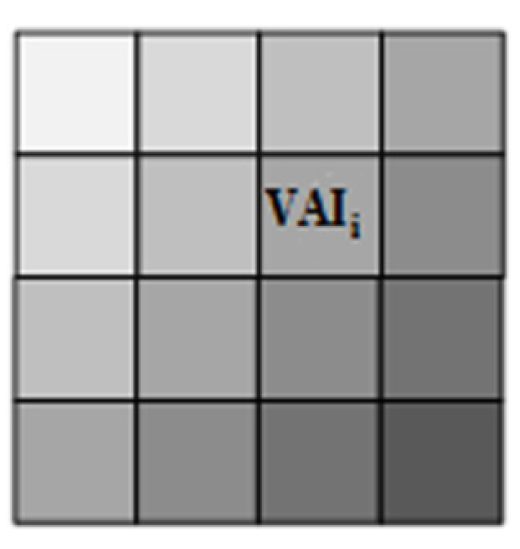
- In the RS-Gash model, for one pixel of satellite image, the VAI is divided into several sub-pixels by Poisson distribution. Each sub-pixel is treated as having homogeneous distribution of VAI when calculating the interception loss of it. The interception loss of the entire pixel is the integration of all sub-pixels by the Poisson distribution probability. The interaction effect among different sub-pixels in one pixel is neglected.

 ) now can be expressed as:
 ), the interception loss of one sub-pixel (Ii) is given by:
), Ii is given by:
), the interception loss of one sub-pixel (Ii) is given by:
), Ii is given by:

3.2. Vegetation Storage Capacity

3.3. Mean Evaporation Rate from Saturated Vegetation

3.4. Heterogeneous Vegetation at Sub-Pixel Scale


4. Study Area and Data
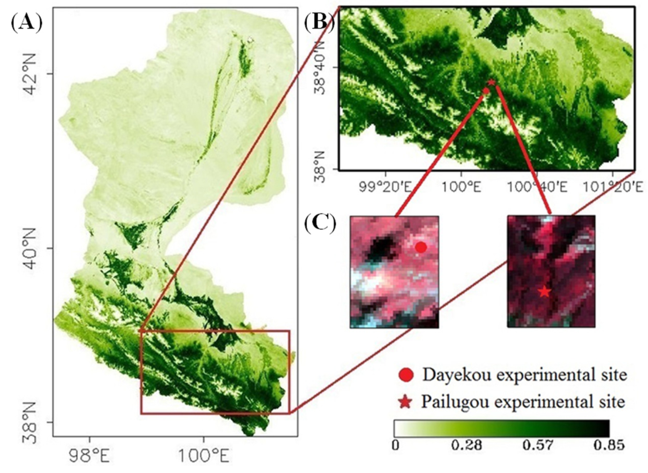
4.1. Study Area


| Features | Dayekou | Pailugou |
|---|---|---|
| Location | (100.258° E, 38.507° N) | (100.295° E, 38.543° N) |
| Elevation (m) | 3128 | 3250 |
| Tree species | picea crassifolia | picea crassifolia |
| Tree average height (m) | 11.5 | 8.4 |
| Density (number of trees ha-1) | 1232 | 1880 |
| Average DBH (diameter at breast height) (cm) | 16.3 | 13.2 |
| canopy cover* | 0.565 | 0.75 |
| Canopy storage* | 0.55 | 1.51 |
| Understorey | With some Bryophyta | With some Bryophyta |
| Plot dimensions (m) | 25 × 25 | 20 × 15 |
| 10 × 15 | ||
| 20 × 25 |
4.2. Remote Sensing Data
4.3. Meteorological Forcing Data
| Variables | Sensor | Manufacturer | Observation accuracy | Observed altitude |
|---|---|---|---|---|
| Tair 24 m | HMP45C | Vaisala | ±0.2 °C | 23.75 m |
| (Helsinki, Finland) | ||||
| Humidity 24 m | HMP45C | Vaisala | ±2% | 23.75 m |
| (Helsinki, Finland) | ||||
| Wind speed 24 m | 034B | MetOne | ±0.11 m/s | 24.00 m |
| (Grants Pass, OR, USA) | ||||
| Pressure | CS105 | Campbell | ±0.5 mb | 0.50 m |
| (Logan, UT, USA) | ||||
| Short-wave radiation (upward and downward) | CM3 | Campbell | ±10% | 19.75 m |
| (Logan, UT, USA) | ||||
| Long-wave Radiation (upward and downward) | CG3 | Campbell | ±10% | 19.75 m |
| (Logan, UT, USA) |
4.4. Validation Data
4.4.1. Dayekou Experimental Site
4.4.2. Pailugou Experimental Site
5. Results and Analysis
5.1. Parameters for the RS-Gash Model
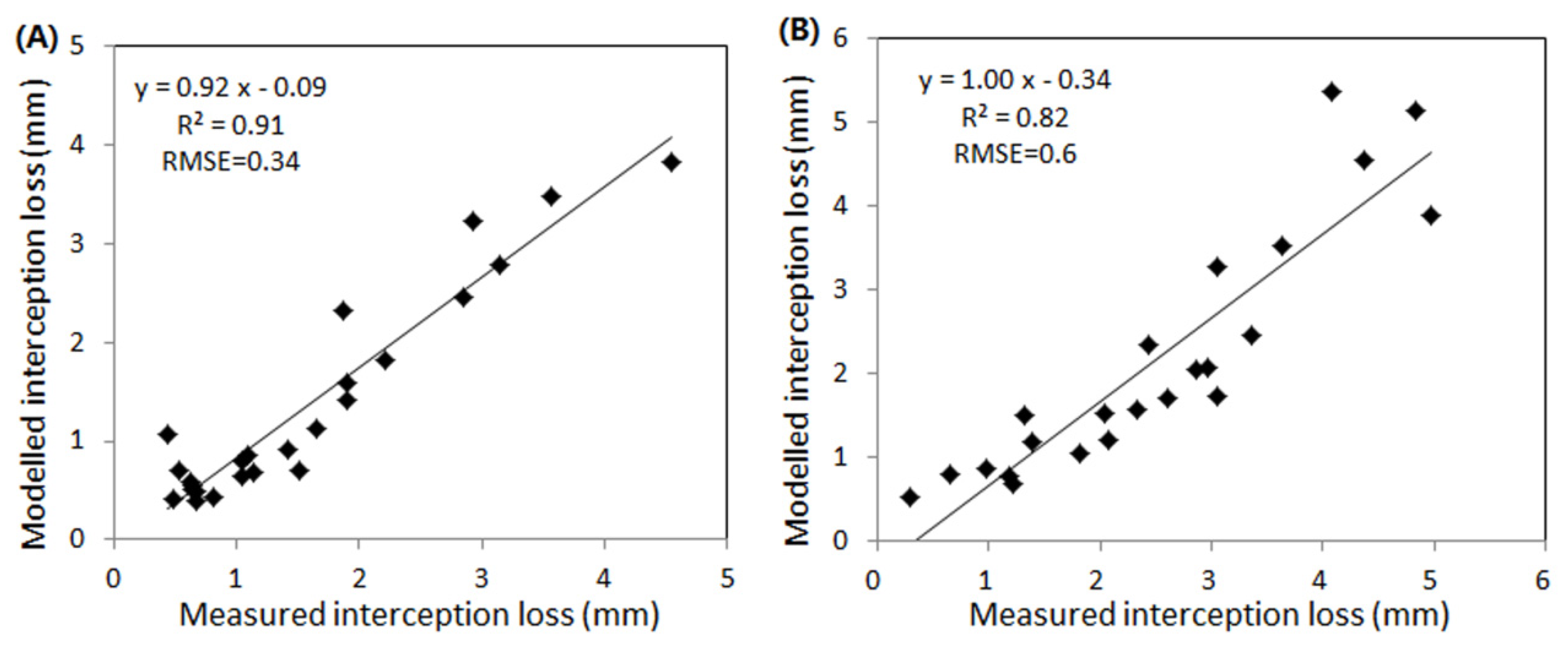
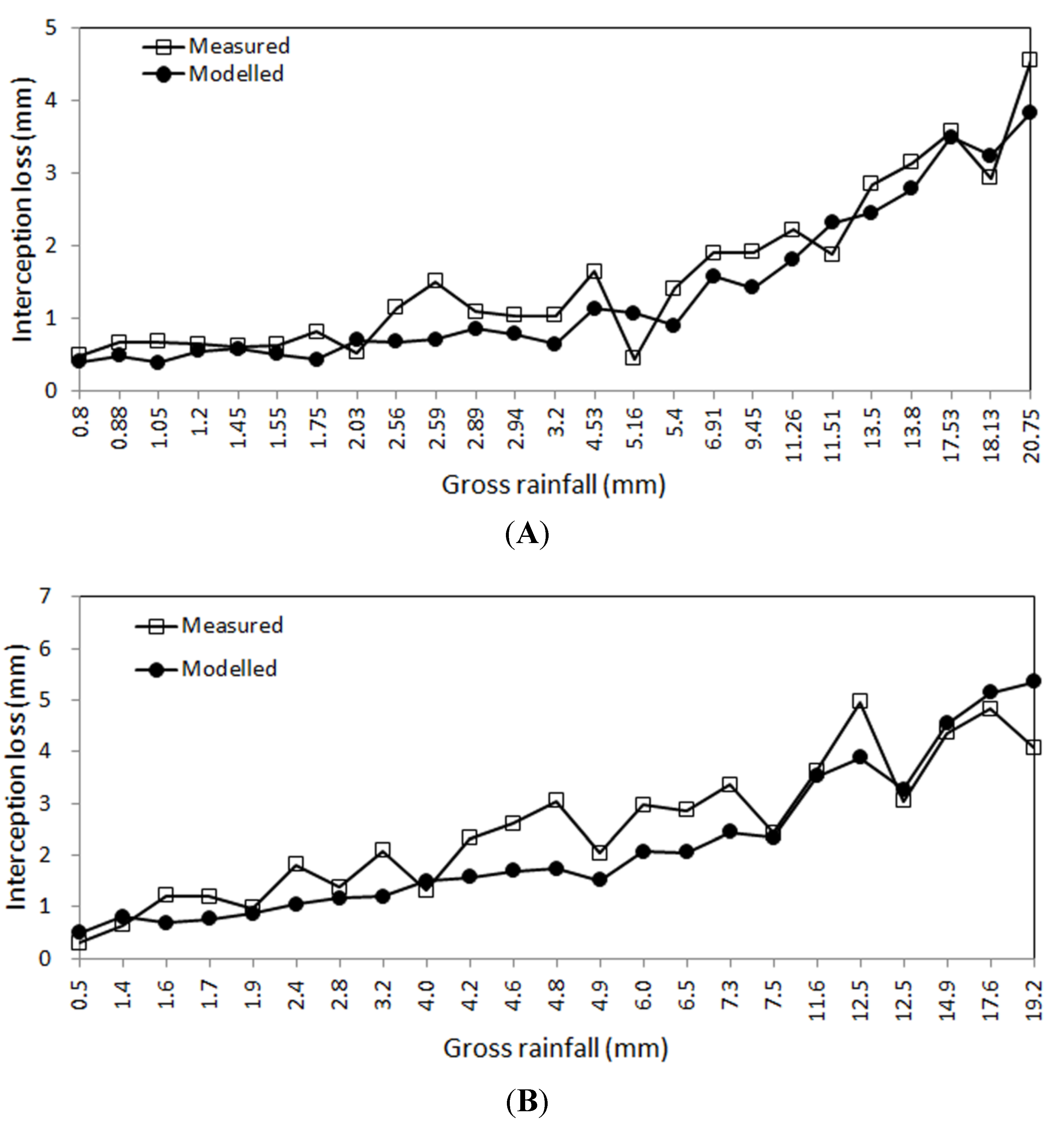
5.2. Field Validation


| Site | Gross rainfall (Pg) (mm) | Modelled | Measured | Relative error (% measured) | ||
|---|---|---|---|---|---|---|
| mm | % Pg | mm | % Pg | |||
| Dayekou | 162.8 | 33.8 | 20.8 | 39.4 | 24.2 | 14.2 |
| Pailugou | 153.5 | 49.7 | 32.4 | 57.5 | 37.5 | 13.6 |
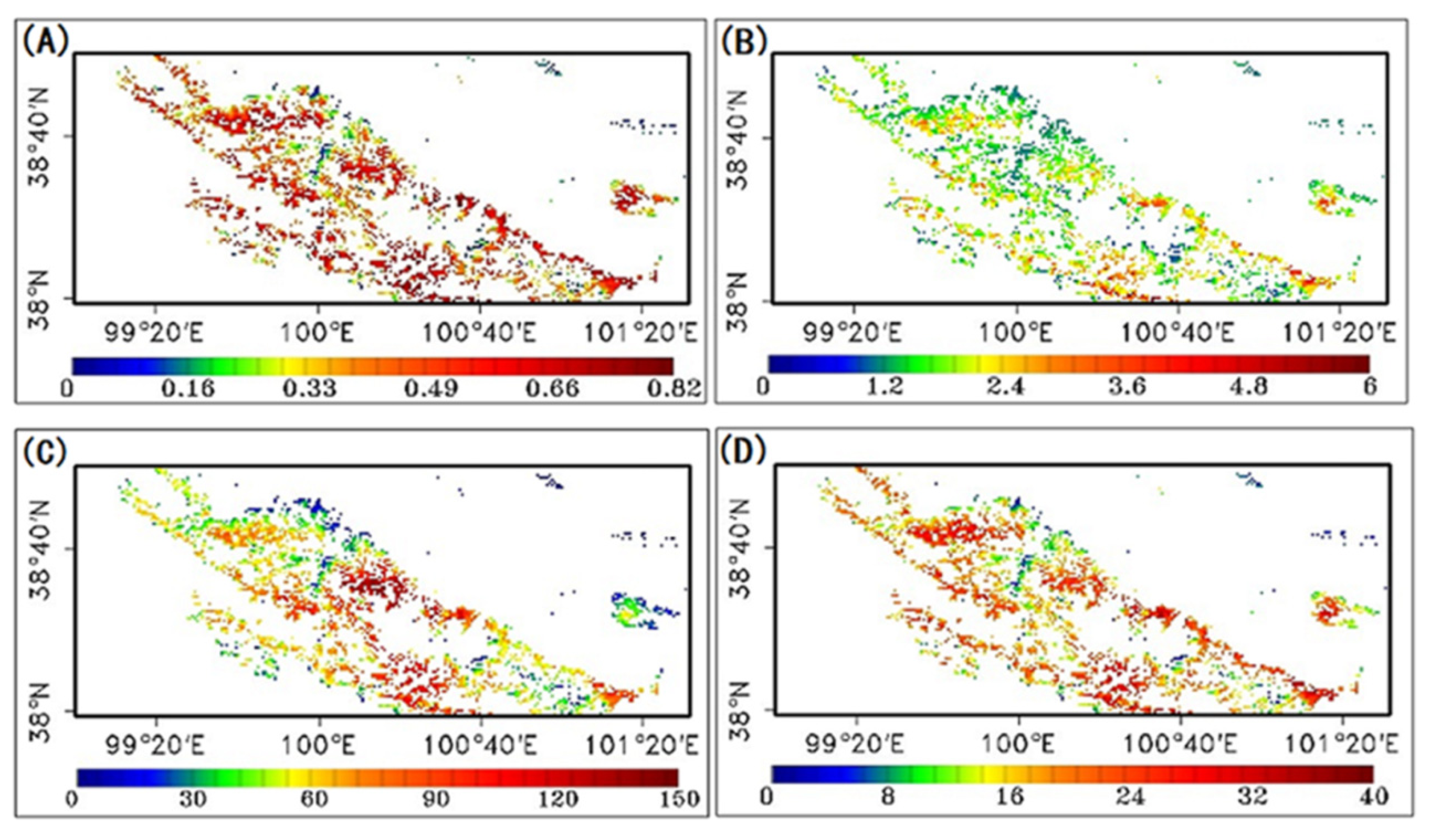
5.3. Interception Loss of Forest at Regional Scale
| Variables | Mean | Standard deviation |
|---|---|---|
| FVC | 0.47 | 0.16 |
| VAI | 1.94 | 0.64 |
| Interception loss (mm) | 61.1 | 26.1 |
| Interception loss (%) | 20.05 | 6.4 |

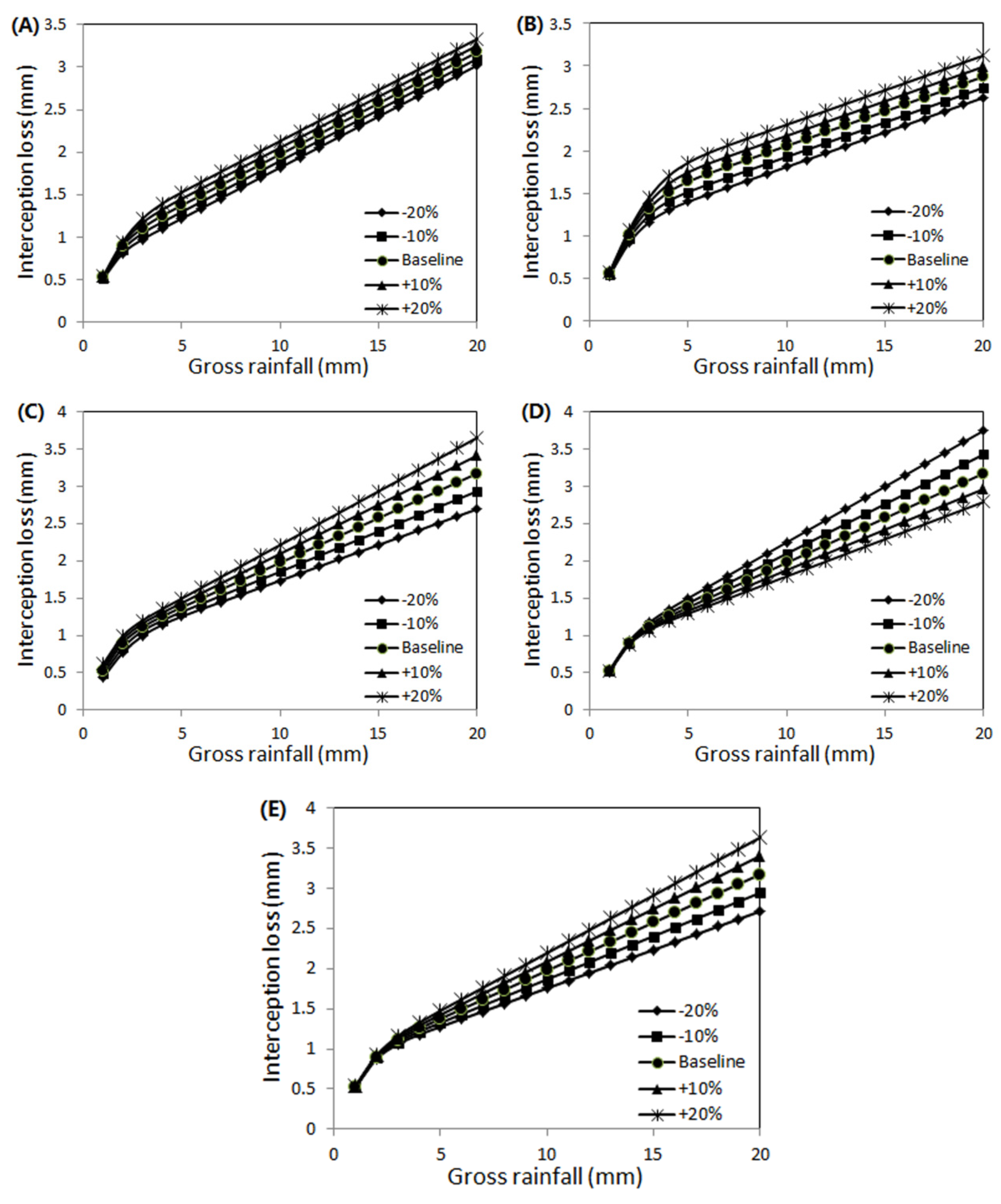
5.4. Sensitivity Analysis of the Model

- For VAI and SV, the error of interception loss was a constant and equal to ΔVAI∙SV or Δsv∙VAI when PG ˃
![Water 06 00993 i013]() ;
; - For FVC、EV、R, the error of interception loss is linear with gross rainfall, and the coefficient is ΔFVC,ΔEV and Δ1/R, when PG ˃
![Water 06 00993 i013]() , respectively;
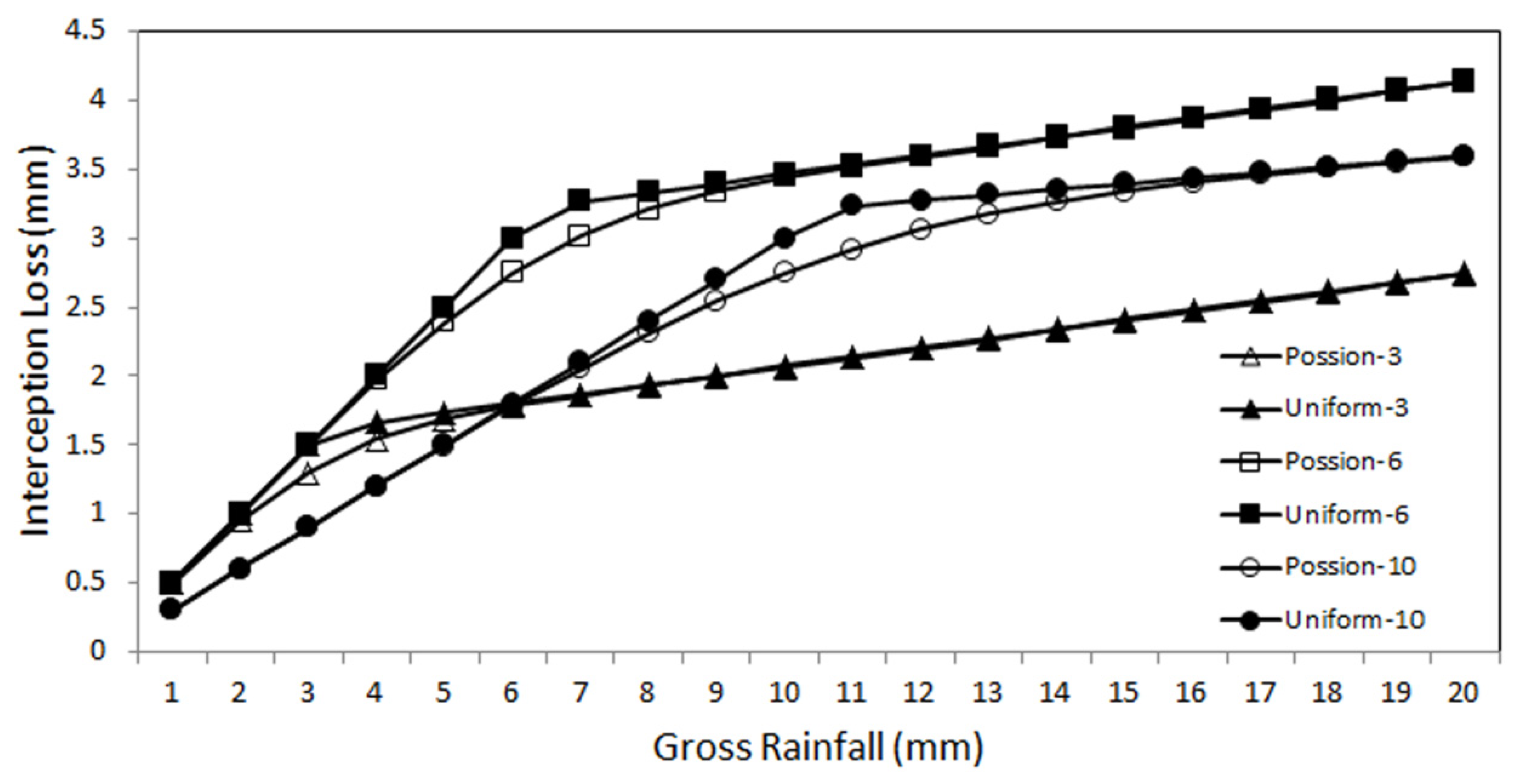
, respectively; - Interception loss using the Poisson distribution is smaller than using uniform distribution, and there are maximum errors near to SV∙VAI/FVC. However the error can be neglected for relatively larger or smaller rainfall. For forest, SV∙VAI/FVC can range from 1 mm to 10 mm, so the heterogeneity of the pixel cannot be neglected, especially for the arid region where the rainfall is dominated by small rainfall.

6. Conclusions
Acknowledgements
Author Contributions
Conflicts of Interest
References
- Scatena, F.N. Watershed scale rainfall interception on 2 forested watersheds in the luquillo mountains of puerto-rico. J. Hydrol. 1990, 113, 89–102. [Google Scholar] [CrossRef]
- Asdak, C.; Jarvis, P.G.; van Gardingen, P.; Fraser, A. Rainfall interception loss in unlogged and logged forest areas of central kalimantan, Indonesia. J. Hydrol. 1998, 206, 237–244. [Google Scholar] [CrossRef]
- Levia, D.F.; Frost, E.E. Variability of throughfall volume and solute inputs in wooded ecosystems. Prog. Phys. Geog. 2006, 30, 605–632. [Google Scholar] [CrossRef]
- Calder, I.R. Water use by forests, limits and controls. Tree Physiol. 1998, 18, 625–631. [Google Scholar] [CrossRef]
- Jackson, I.J. Relationships between rainfall parameters and interception by tropical forest. J. Hydrol. 1975, 24, 215–238. [Google Scholar] [CrossRef]
- Gash, J.H. An analytical model of rainfall interception by forests. Q. J. Roy. Meteor. Soc. 1979, 105, 43–55. [Google Scholar] [CrossRef]
- Rutter, A.J.; Robins, P.C.; Morton, A.J.; Kershaw, K.A. Predictive model of rainfall interception in forests.1. Derivation of model from observations in a plantation of corsican pine. Agr. Meteorol. 1972, 9, 367–384. [Google Scholar]
- Gash, J.H.C.; Lloyd, C.R.; Lachaud, G. Estimating sparse forest rainfall interception with an analytical model. J. Hydrol. 1995, 170, 79–86. [Google Scholar] [CrossRef]
- Liu, S.G. Estimation of rainfall storage capacity in the canopies of cypress wetlands and slash pine uplands in North-Central Florida. J. Hydrol. 1998, 207, 32–41. [Google Scholar] [CrossRef]
- Van Dijk, A.I.J.M.; Bruijnzeel, L.A. Modelling rainfall interception by vegetation of variable density using an adapted analytical model. Part 1. Model description. J. Hydrol. 2001, 247, 230–238. [Google Scholar] [CrossRef]
- Murakami, S. A proposal for a new forest canopy interception mechanism: Splash droplet evaporation. J. Hydrol. 2006, 319, 72–82. [Google Scholar] [CrossRef]
- Muzylo, A.; Llorens, P.; Valente, F.; Keizer, J.J.; Domingo, F.; Gash, J.H.C. A review of rainfall interception modelling. J. Hydrol. 2009, 370, 191–206. [Google Scholar] [CrossRef]
- Bastiaanssen, W.G.M.; Cheema, M.J.M.; Immerzeel, W.W.; Miltenburg, I.J.; Pelgrum, H. Surface energy balance and actual evapotranspiration of the transboundary indus basin estimated from satellite measurements and the etlook model. Water Resour. Res. 2012, 48, W11512. [Google Scholar]
- Von Hoyningen, H.J. Die interception des niederschlags in landwirtschaftlichen bestanden. Schriftenr. DVWK 1983, 57, 1. [Google Scholar]
- Mu, Q.Z.; Zhao, M.S.; Running, S.W. Improvements to a modis global terrestrial evapotranspiration algorithm. Remote Sens. Environ. 2011, 115, 1781–1800. [Google Scholar] [CrossRef]
- Hutjes, R.W.A.; Wierda, A.; Veen, A.W.L. Rainfall interception in the tai forest, ivory-coast—Application of 2 simulation-models to a humid tropical system. J. Hydrol. 1990, 114, 259–275. [Google Scholar] [CrossRef]
- Valente, F.; David, J.S.; Gash, J.H.C. Modelling interception loss for two sparse eucalypt and pine forests in central portugal using reformulated rutter and gash analytical models. J. Hydrol. 1997, 190, 141–162. [Google Scholar] [CrossRef]
- Schellekens, J.; Scatena, F.N.; Bruijnzeel, L.A.; Wickel, A.J. Modelling rainfall interception by a lowland tropical rain forest in northeastern puerto rico. J. Hydrol. 1999, 225, 168–184. [Google Scholar] [CrossRef]
- Motahari, M.; Attarod, P.; Pypker, T.G.; Etemad, V.; Shirvany, A. Rainfall interception in a pinus eldarica plantation in a semi-arid climate zone: An application of the gash model. J. Agr. Sci. Tech. Iran. 2013, 15, 981–994. [Google Scholar]
- Van Dijk, A.I.J.M.; Bruijnzeel, L.A. Modelling rainfall interception by vegetation of variable density using an adapted analytical model. Part 2. Model validation for a tropical upland mixed cropping system. J. Hydrol. 2001, 247, 239–262. [Google Scholar] [CrossRef]
- Zeng, X.B.; Shaikh, M.; Dai, Y.J.; Dickinson, R.E.; Myneni, R. Coupling of the common land model to the ncar community climate model. J. Clim. 2002, 15, 1832–1854. [Google Scholar] [CrossRef]
- Miralles, D.G.; Gash, J.H.; Holmes, T.R.H.; de Jeu, R.A.M.; Dolman, A.J. Global canopy interception from satellite observations. J. Geophys. Res. Atmos. 2010, 115. [Google Scholar] [CrossRef]
- Pitman, J.I. Rainfall interception by bracken in open habitats—Relations between leaf-area, canopy storage and drainage rate. J. Hydrol. 1989, 105, 317–334. [Google Scholar] [CrossRef]
- Llorens, P.; Gallart, F. A simplified method for forest water storage capacity measurement. J. Hydrol. 2000, 240, 131–144. [Google Scholar] [CrossRef]
- Aston, A.R. Rainfall interception by 8 small trees. J. Hydrol. 1979, 42, 383–396. [Google Scholar] [CrossRef]
- Lankreijer, H.; Lundberg, A.; Grelle, A.; Lindroth, A.; Seibert, J. Evaporation and storage of intercepted rain analysed by comparing two models applied to a boreal forest. Agr. Forest Meteorol. 1999, 98–99, 595–604. [Google Scholar]
- Monteith, J.L. Evaporation and environment. Symp. Soc. Exp. Biol. 1965, 19, 205–223. [Google Scholar]
- Myneni, R.B.; Ross, J.; Asrar, G. A review on the theory of photon transport in leaf canopies. Agr. Forest Meteorol. 1989, 45, 1–153. [Google Scholar] [CrossRef]
- Li, X.; Li, X.W.; Li, Z.Y.; Ma, M.G.; Wang, J.; Xiao, Q.; Liu, Q.; Che, T.; Chen, E.X.; Yan, G.J.; et al. Watershed allied telemetry experimental research. J. Geophys. Res. Atmos. 2009, 114. [Google Scholar] [CrossRef]
- Ran, Y.H.; Li, X.; Lu, L.; Li, Z.Y. Large-scale land cover mapping with the integration of multi-source information based on the dempster-shafer theory. Int. J. Geogr. Inf. Sci. 2012, 26, 169–191. [Google Scholar] [CrossRef]
- Tropical Rainfall Measuring Mission (TRMM). Available online: http://trmm.gsfc.nasa.gov/ (accessed on 16 April 2014).
- Herbst, M.; Rosier, P.T.W.; McNeil, D.D.; Harding, R.J.; Gowing, D.J. Seasonal variability of interception evaporation from the canopy of a mixed deciduous forest. Agr. Forest Meteorol. 2008, 148, 1655–1667. [Google Scholar]
- Jia, L.; Shang, H.; Hu, G.; Menenti, M. Phenological response of vegetation to upstream river flow in the heihe rive basin by time series analysis of modis data. Hydrol. Earth Syst. Sci. 2011, 15, 1047–1064. [Google Scholar] [CrossRef]
© 2014 by the authors; licensee MDPI, Basel, Switzerland. This article is an open access article distributed under the terms and conditions of the Creative Commons Attribution license (http://creativecommons.org/licenses/by/3.0/).
Share and Cite
Cui, Y.; Jia, L. A Modified Gash Model for Estimating Rainfall Interception Loss of Forest Using Remote Sensing Observations at Regional Scale. Water 2014, 6, 993-1012. https://doi.org/10.3390/w6040993
Cui Y, Jia L. A Modified Gash Model for Estimating Rainfall Interception Loss of Forest Using Remote Sensing Observations at Regional Scale. Water. 2014; 6(4):993-1012. https://doi.org/10.3390/w6040993
Chicago/Turabian StyleCui, Yaokui, and Li Jia. 2014. "A Modified Gash Model for Estimating Rainfall Interception Loss of Forest Using Remote Sensing Observations at Regional Scale" Water 6, no. 4: 993-1012. https://doi.org/10.3390/w6040993