Retention and Curve Number Variability in a Small Agricultural Catchment: The Probabilistic Approach


Abstract
:1. Introduction


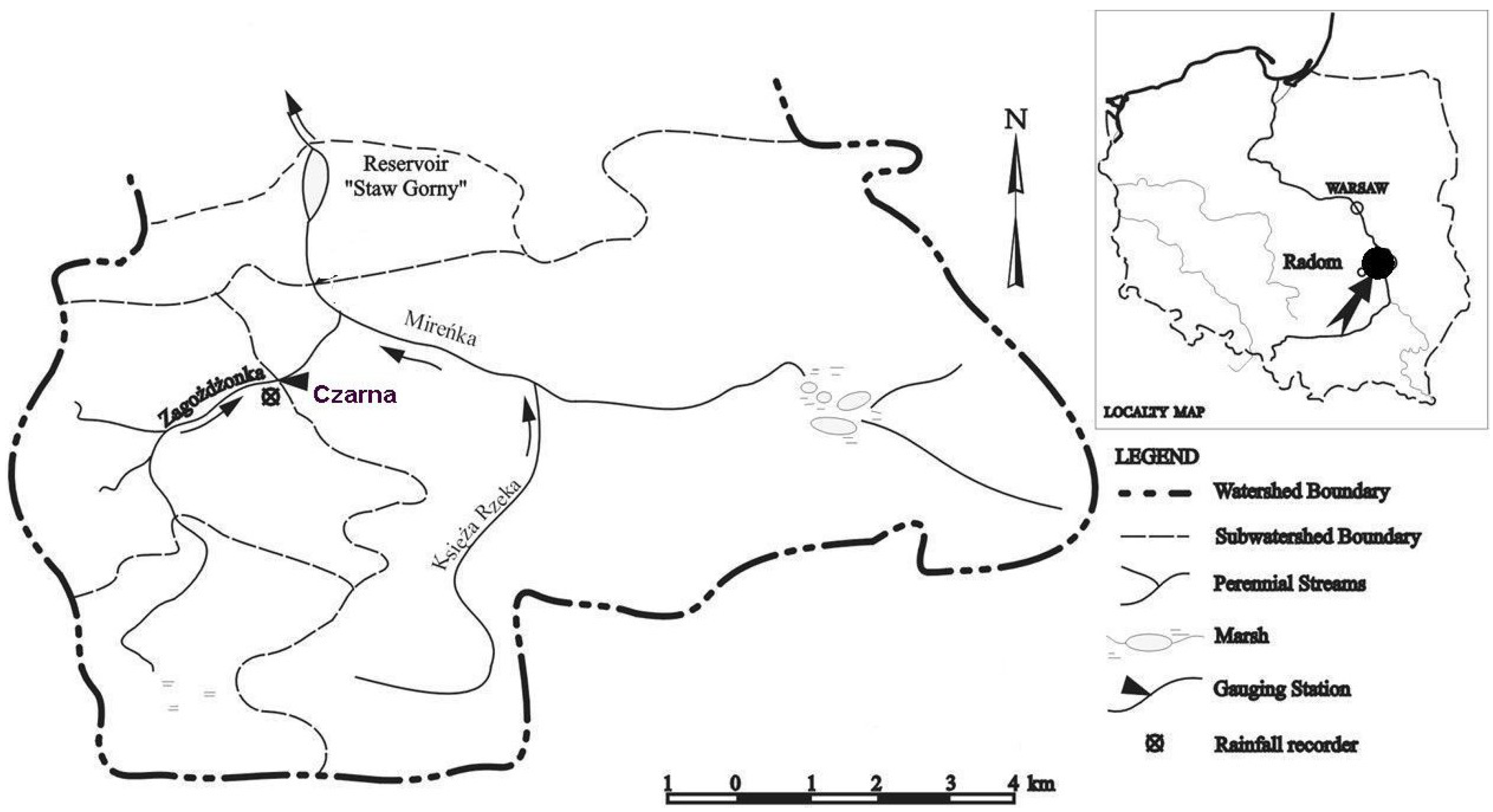
2. Watershed Characteristics

3. Material and Methods


3.1. Identification of the Theoretical Distribution
 , as in Equation (5). Then, q, the inverse function of p, is expressed as q(y) = 254(
  − 1) (Equation (2)). The relationship between the densities is given by
  [29]. If the distribution of S is from a known family (e.g., lognormal, GEV, Weibull, etc.); then, this formula is impractical, being computationally highly complex and not leading to a distribution from a known family. This is because the distributions of S and CN were identified separately in this paper.
 . This value is the estimate of θ in the MLE method. Often, ln L is considered, instead of L, to provide an effective method for estimation.


3.2. Confidence Intervals and ARC


4. Results and Discussion

| Sample | Mean Value | Median | Coeff. of Var. (%) | Range | Skewnes | |||||
|---|---|---|---|---|---|---|---|---|---|---|
| S | CN | S | CN | S | CN | S | CN | S | CN | |
| A | 81.1 | 75.8 | 83.6 | 75.2 | 59.1 | 14.1 | 233.5 | 44 | 1 | −0.2 |
| B | 62.3 | 81.1 | 63.6 | 80 | 51.8 | 10 | 124 | 29.9 | 0.4 | −0.05 |
| C | 130.2 | 66.1 | 127.2 | 66.6 | 36.1 | 11.8 | 175.8 | 27.3 | 1 | −0.3 |
4.1. Assessment of the Accuracy of CNtab and the ARCs of Hawkins under Very Heavy and Moderate Rainfall
| GEV | N | GLO | WE | LN | G | GEV | N | GLO | WE | LN | G | ||
|---|---|---|---|---|---|---|---|---|---|---|---|---|---|
| W for S | AIC for S | ||||||||||||
| A | 20.0 | × | 16.0 | 33.2 | 33.1 | 33.1 | 364.8 | × | 364.8 | 365.1 | 364.4 | 364.8 | |
| B | 26.2 | × | 25.2 | × | 34.9 | × | 219.2 | × | 219.6 | × | 218.7 | × | |
| C | 26.3 | × | 19.7 | 29.8 | 29.6 | 30.7 | 130.6 | × | 130.7 | 130.9 | 128.6 | 130.8 | |
| W for 100-CN | AIC for 100-CN | ||||||||||||
| A | 13.8 | 17.5 | 19.1 | × | × | × | 262.12 | 260.1 | 263.8 | × | × | × | |
| B | 25.6 | 27.4 | 27.4 | × | × | × | 158.9 | 157.5 | 160.7 | × | × | × | |
| C | 22.3 | 25.5 | 24.3 | 37.4 | 33.1 | 26.5 | 88.0 | 86.3 | 88.6 | 88.7 | 88.2 | 88.1 | |
| A | B | C | |||||||
|---|---|---|---|---|---|---|---|---|---|
| Characteristic | GEV | N | GLO | GEV | N | GLO | GEV | N | GLO |
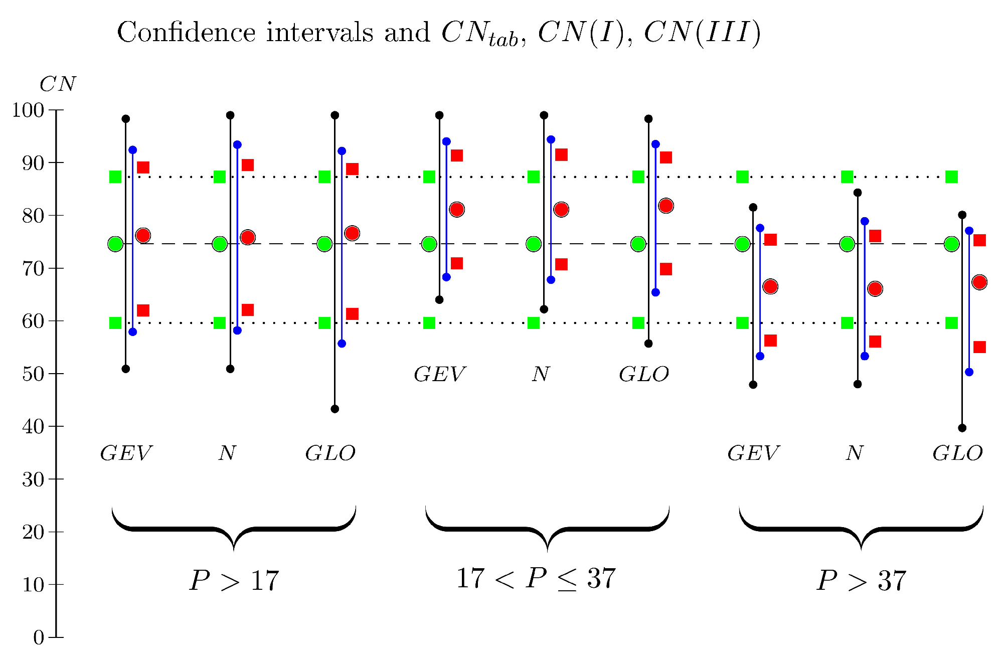
| median | 76.2 | 75.8 | 76.6 | 81.1 | 81.1 | 81.8 | 66.5 | 66.1 | 67.3 |
| CN (I)Hjel | 62.0 | 62.1 | 61.3 | 70.9 | 70.7 | 69.8 | 56.3 | 56.1 | 55.0 |
| CN (III)Hjel | 89.1 | 89.5 | 88.8 | 91.3 | 91.5 | 91.0 | 75.4 | 76.1 | 75.3 |
| a95%(∗) | 57.9 | 58.2 | 55.7 | 68.3 | 67.8 | 65.4 | 53.3 | 53.3 | 50.3 |
| b95%(∗) | 92.4 | 93.4 | 92.2 | 94.0 | 94.4 | 93.5 | 77.6 | 78.9 | 77.1 |
| a99% | 50.9 | 50.9 | 43.3 | 64.0 | 62.2 | 55.7 | 47.9 | 48.0 | 39.7 |
| b99% | 98.3 | 99.0 | 99.0 | 99.0 | 99.0 | 98.3 | 81.5 | 84.3 | 80.1 |

4.2. Assessment of the Applicability of the ARCs of Hawkins
5. Conclusions
- instead of CN (I)Haw = 59.6 and for a rainfall depth not much higher than 17 mm, consider a value between 70 or 71, which is near CN (I)Hjel for moderate rainfall,
- instead of CN (III)Haw = 87.3 and for a very high rainfall depth, consider a value between 75 or76, which is near CN (III)Hjel for stormy rainfall.
Acknowledgments
Author Contributions
Conflicts of Interest
References
- Banasik, K. Catchment responses to heavy rainfall events in a changing environment. In Prediction and Reduction of Diffuse Pollution, Solid Emission and Extreme Flows from Rural Areas—Case Study of Small Agricultural Catchments; Banasik, K., Øygarden, L., Hejduk, L., Eds.; SGGW Press: Warsaw, Poland, 2011; pp. 7–25. [Google Scholar]
- Arnell, N. Hydrology and Global Environmental Change; Prentice Hall: Essex, UK, 2002. [Google Scholar]
- Gaál, L.; Szolgay, J.; Lapin, M.; Faško, P. Hybrid approach to delineation of homogeneous regions for regional precipitation frequency analysis. J. Hydrol. Hydromech. 2009, 57, 226–249. [Google Scholar]
- Mishra, S.K.; Tyagi, J.V.; Singh, V.P.; Singh, R. SCS-CN-based modeling of sediment yield. J. Hydrol. 2006, 324, 301–322. [Google Scholar] [CrossRef]
- Arnold, J.G.; Williams, J.R.; Srinivasan, R.; King, K.W. SWAT: Soil Water Assessment Tool; Texas Agricultural Experiment Station: Blackland Research Center, Texas A&M University, Temple, TX, USA, 1995. [Google Scholar]
- ASCE. Curve Number Hydrology: State of the Practice; Hawkins, R.H., Ward, T.J., Woodward, D.E., van Mullem, J.A., Eds.; American Society of Civil Engineers: Reston, VA, USA, 2009. [Google Scholar]
- USDA NRCS. National Engineering Handbook: Part 630—Hydrology; USDA Soil Conservation Service: Washington, DC, USA, 2004. [Google Scholar]
- Hawkins, R. Improved prediction of storm runoff in mountain watersheds. J. Irrig. Drain. Div. 1973, 99, 519–523. [Google Scholar]
- Hawkins, R. Runoff curve numbers from partial area watersheds. J. Irrig. Drain. Div. 1979, 105, 375–389. [Google Scholar]
- Hawkins, R.; Hjelmfelt, J.A.; Zevenbergen, A. Runoff probability, storm depth and curve numbers. J. Irrig. Drain. Div. 1985, 111, 330–340. [Google Scholar] [CrossRef]
- Mishra, S.K.; Singh, V.P.; Sansalone, J.J.; Aravamuthan, V. A modified SCS-CN method: Characterization and Testing. Water Resour. Manag. 2003, 17, 37–68. [Google Scholar] [CrossRef]
- Babu, P.S.; Mishra, S.K. Improved SCS-CN-Inspired Model. J. Hydrol. Eng. 2012, 17, 1164–1172. [Google Scholar] [CrossRef]
- Hjelmfelt, A. Investigation of curve number procedure. J. Hydraul. Eng. 1991, 117, 725–737. [Google Scholar] [CrossRef]
- McCuen, R. Approach to confidence interval estimation for curve numbers. J. Hydrol. Eng. 2002, 7, 43–48. [Google Scholar] [CrossRef]
- Schneider, L.E.; McCuen, R. Statistical Guidelines for Curve Number Generation. J. Irrig. Drain. Eng. 2005, 131, 282–290. [Google Scholar] [CrossRef]
- Tedela, N.M.; McCutcheon, S.C.; Rasmussen, T.C.; Tollner, E.W. Evaluation and Improvements of the Curve Number Method of Hydrological Analysis on Selected Forested Watersheds of Georgia. The University of Georgia, report submitted to Georgia Water Resources Institute. Available online: http://water.usgs.gov/wrri/07grants/progress/2007GA143B.pdf (accessed on 25 October 2013).
- Bondelid, T.; McCuen, R.; Jackson, T. Sensitivity of SCS Models to Curve Number Variation. JAWRA 1982, 18, 111–116. [Google Scholar]
- Epps, T.H.; Hitchcock, D.R.; Jayakaran, A.D.; Loflin, D.R.; Williams, T.M.; Amatya, D.M. Curve Number derivation for watersheds draining two headwater streams in lower coastal plain South Carolina, USA. JAWRA 2013, 49, 1284–1295. [Google Scholar]
- Hawkins, R. Asymptotic determination of curve numbers from data. J. Irrig. Drain. Div. 1993, 119, 334–345. [Google Scholar] [CrossRef]
- Banasik, K.; Ignar, S. Estimation of effective rainfall using the SCS method on the base of measured rainfall and runoff. Rev. Geophys. 1983, XXVII, 401–408. (In Polish) [Google Scholar]
- Banasik, K.; Woodward, D. Empirical determination of runoff curve number for a small agricultural watershed in Poland. Proceedings of the 2 Joint Federal Interagency Conference, Las Vegas, NV, USA, 27 June–1 July 2010; pp. 1–11. Available online: http://acwi.gov/sos/pubs/2ndJFIC/ Contents/10E_Banasik_28_02_10.pdf (accessed on 25 October 2013).
- Tedela, N.H.; McCutcheon, S.C.; Rasmussen, T.C.; Hawkins, R.H.; Swank, W.T.; Campbell, J.L.; Adams, M.B.; Jackson, R.C.; Tollner, E.W. Runoff Curve Numbers for 10 Small Forested Watersheds in the Mountains of the Eastern United States. J. Hydrol. Eng. 2012, 17, 1188–1198. [Google Scholar] [CrossRef]
- Banasik, K. Sedimentgraph model of rainfall event in a small agricultural watershed. In Treaties and Monographs; SGGW Press: Warsaw, Poland, 1994. (In Polish) [Google Scholar]
- Banasik, K.; Hejduk, L. Long-term Changes in Runoff from a Small Agricultural Catchment. Soil Water Res. 2012, 2, pp. 64–72. Available online: http://www.agriculturejournals.cz/publicFiles/64803.pdf (accessed on 25 October 2013).
- Banasik, K.; Hejduk, L. Flow Duration Curves for Two Small Catchments with Various Records in Lowland Part of Poland. Annu. Set Environ. Prot. 2013, 15, 287–300. [Google Scholar]
- Chow, V.T. Handbook of Applied Hydrology: A Compendium of Water-Resources Technology (Section 14 Runoff); McGraw-Hill Book Company: New York, NY, USA, 1964. [Google Scholar]
- Mitchell, J.K.; Banasik, K.; Hirschi, M.C.; Cooke, R.A.C.; Kalita, P. There is not always surface runoff and sediment transport. In Soil Erosion Research for the 21st Century; Ascough, J.C., Flanagan, D.C., Eds.; ASAE: St. Joseph, MI, USA, 2001; pp. 676–678. [Google Scholar] [CrossRef]
- USDA Soil Conservation Service (SCS). National Engineering Handbook (Section 4 Hydrology); USDA SCS: Washington, DC, USA, 1954. [Google Scholar]
- Billingsley, P. Probability and Measure; John Wiley & Sons: New York, NY, USA; Chichester, UK; Brisbane, Australia; Toronto, ON, Canada, 1979. [Google Scholar]
- Barra, J.R. Notions fondamentales de statistique mathèmatique; Dunod: Paris, France, 1971. [Google Scholar]
- Lehmann, E.L.; Casella, G. Theory of Point Estimation, 2nd ed.; Springer: New York, NY, USA, 1998; Toronto, ON, Canada, 1979.
- Lehmann, E.L.; Romano, J.P. Testing Statistical Hypotheses, 3rd ed.; Springer Texts in Statistics; Springer: New York, USA, 2005. [Google Scholar]
- Stephens, M.A. Tests Based on EDF Statistics, in Goodness-of-Fit Techniques; Marcel Dekker: New York, NY, USA, 1986. [Google Scholar]
- Anderson, T.W.; Darling, D.A. A Test of Goodness of Fit. J. Am. Stat. Assoc. 1954, 49, 765–769. [Google Scholar] [CrossRef]
- Laio, F. Cramer-von Mises and Anderson Darling goodness of fit tests for extreme value distributions with unknown parameters. Water Resour. Res. 2004, 40. [Google Scholar] [CrossRef]
- Shapiro, S.S.; Wilk, M.B. An analysis of variance test for normality (complete samples). Biometrika 1965, 52, 591–611. [Google Scholar] [CrossRef]
- DVWK. Regeln 101/1999 Estimation of Design Discharges. Guidelines; Paul Parey: Hamburg, Germany, 1999. (In German) [Google Scholar]
- Akaike, H. A new look at the statistical model identification. IEEE Trans. Autom. Control 1974, 19, 716–723. [Google Scholar] [CrossRef]
- Banasik, K.; Byczkowski, A. Probable annual floods in a small lowland river estimated with the use of various sets of data. Ann. Wars. Univ. Life Sci.-SGGW Land Reclam. 2007, 38, 3–10. [Google Scholar]
- Laio, F.; Baldassare, G.; Montanari, A. Model selection techniques for the frequency analysis of hydrological extremes. Water Resour. Res. 2009, 45. [Google Scholar] [CrossRef]
- Bonta, J.V. Determination of watershed curve number using derived distributions. J. Irrig. Drain. Div. 1997, 123, 28–36. [Google Scholar] [CrossRef]
© 2014 by the authors; licensee MDPI, Basel, Switzerland. This article is an open access article distributed under the terms and conditions of the Creative Commons Attribution license (http://creativecommons.org/licenses/by/3.0/).
Share and Cite
Banasik, K.; Rutkowska, A.; Kohnová, S. Retention and Curve Number Variability in a Small Agricultural Catchment: The Probabilistic Approach. Water 2014, 6, 1118-1133. https://doi.org/10.3390/w6051118
Banasik K, Rutkowska A, Kohnová S. Retention and Curve Number Variability in a Small Agricultural Catchment: The Probabilistic Approach. Water. 2014; 6(5):1118-1133. https://doi.org/10.3390/w6051118
Chicago/Turabian StyleBanasik, Kazimierz, Agnieszka Rutkowska, and Silvia Kohnová. 2014. "Retention and Curve Number Variability in a Small Agricultural Catchment: The Probabilistic Approach" Water 6, no. 5: 1118-1133. https://doi.org/10.3390/w6051118