The Effects of Surface Debris Diversion Devices on River Hydrodynamic Conditions and Implications for In-Stream Hydrokinetic Development

Abstract

Floating objects designed to divert woody debris—known as debris diversion devices—can protect hydrokinetic turbines deployed in rivers; they also change the hydrodynamic conditions of a river, at least locally. Modifications associated with velocity adjustments in both magnitude and direction would be expected. Thus, one could assume that extra macro-turbulent levels would be found immediately behind a device and downstream of that location. This article presents a set of cross-sectional and longitudinal velocity measurements carried out to quantify these effects. Results show important changes in the velocity components. In addition, significant changes in the vorticity field, calculated along cross-sectional profiles, demonstrate the role of a submerged chain used to maintain the debris diversion device in place. More importantly, findings suggest that hydrokinetic turbines should not be installed in a river’s central area behind a debris diversion device, due to the additional turbulence created by the submerged chain.

1. Introduction

The global increase in energy demand has promoted the study of alternative and renewable energy sources, such as in-stream hydrokinetic energy [1]. The current technology is still considered pre-commercial [2], and no devices are currently deployed in Alaska, USA [3]. Several recent studies have focused on Alaska’s resource assessment [3,4,5], river turbulence [6,7] and hydro-sedimentological river conditions [8]; however, no studies have yet been reported on the influence of manufactured floating objects on river hydrodynamic conditions.

One expects the presence of large woody debris (LWD) in the water when a stream runs through a wooded landscape. This debris can create hazardous conditions for navigation and for objects deployed in rivers. The importance of LWD on fish habitat and fish passage, river hydraulics and river morphology has been reported by several researchers [9,10,11] and many others. Studies on river hydraulics have accounted for local and reach-averaged scales [12]. Laboratory experiments have been carried out to investigate motion thresholds and the transport and deposition of logs [13,14]. Floating debris logs create additional friction, which reduces average flow velocity and locally increases the water level [11]. Recently published work, based on complex numerical simulations [15,16], has focused on stream restoration. It is expected that a similar approach could be applied to floating structures deployed in the stream.

Parallel to previous studies, researchers have focused on designing mechanical devices used to remove LWD from streams to protect, for instance, water inlets, bridge piers and turbines. Reviews of existing mechanisms have been provided [17,18,19].

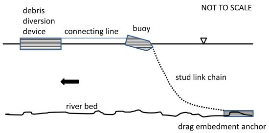
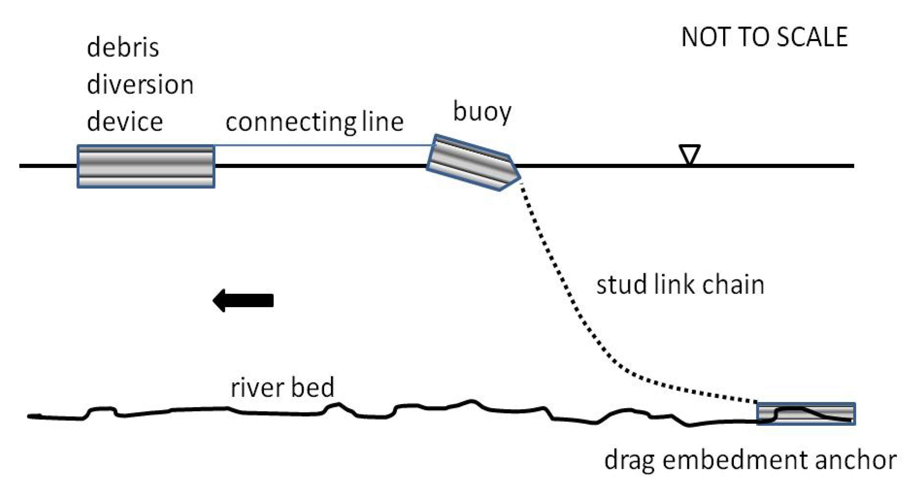
This article presents basic hydrodynamic changes along selected river cross-sections located downstream of a debris diversion boom installed in the Tanana River near Nenana, Alaska. This debris diversion device (DDD), which diverts floating debris, consists of two pontoons connected at one end and separated at the other end to form an angle with its apex pointing upstream [3].

2. Device Configurations and Field Equipment

The DDD deployed in the Tanana River (coordinates 64.5609° N, 149.065° W) consisted of two metallic pontoons 600 cm-long, 60 cm-deep (approximately 30 cm submerged in the water) and 60 cm-wide. The pontoons were joined at the upstream end and separated at the downstream end to form an angle. This angle could be changed from a minimum opening of approximately 30 degrees to a maximum opening of roughly 90 degrees. The DDD apex was connected to a buoy located upstream by a suspended nylon line. The buoy consisted of a 2000-liter steel tank, with the following dimensions: diameter = 117 cm; length = 188 cm. A 117 cm-long cone was added to the upstream end of the buoy. This side of the cone was connected to a drag embedment anchor by a stud link chain. The anchor weight was approximately 1,500 kg; the chain’s stock diameter was 2.22 cm, with a total geometric expression (i.e., distance perpendicular to the water flow direction) of 8 cm. Thus, one could expect significant perturbations along the water column generated by the chain. A sketch of the field configuration is shown in Figure 1.

An acoustic Doppler current profiler (ADCP), Rio Grande 1200 kHz, manufactured by RD Instruments, was mounted on an aluminum boat and used to carry out velocity measurements. Two GPS units (one on the boat; one on the ground near the riverbank) and two radios provided real-time kinematic (RTK) correction to the measurements. During the measurements, the ADCP update rate was set at 0.4 seconds. The transducer was situated 0.25 m below the water surface. Hence, the first bin was located 0.86 m below the water surface. The bin size was 0.25 m. Thus, the water depth was “partitioned” every 0.25 m, starting at 0.86 m from the water surface.

Figure 1. Sketch of the field configuration.

Figure 1. Sketch of the field configuration.

3. Methodology

To identify the main changes in the river’s hydrodynamic conditions due to the DDD, buoy and anchor, two types of field measurements were performed: (1) cross-sectional velocity profiles and (2) longitudinal velocity profiles. The purpose of these measurements was to provide insights into velocity changes in both directions.

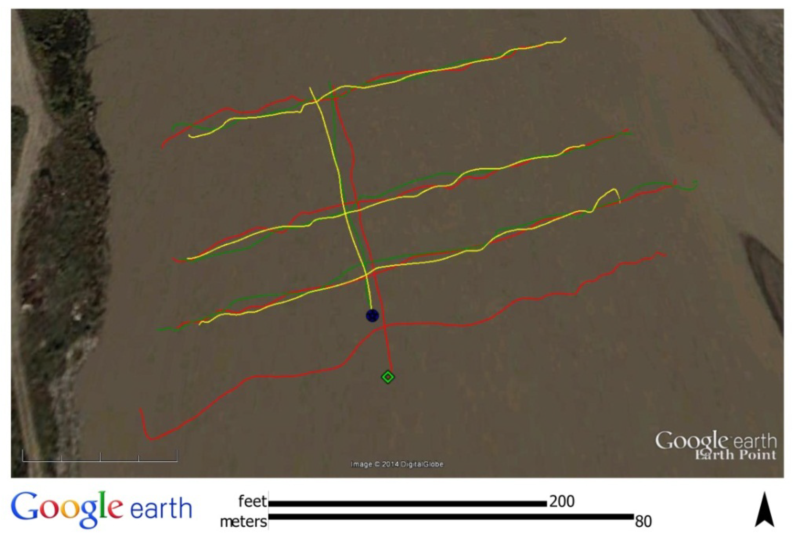
Markers in each riverbank were established to delineate several transects (i.e., two markers per transect per bank) located downstream of the buoy and DDD. These transects were approximately perpendicular to the stream. The markers were used by the boat driver as guides to maintain the course across the river during the velocity measurements along transects. The distance between transects was 20 m. While additional transects were defined in the field, only four transects are reported here. These transects covered a length of 80 m in the downstream direction (or approximately 12-times the average water depth along the river reach). One transect was located downstream of the buoy, and three transects were located downstream of the DDD. Figure 2 shows the spatial distribution of transects.

All but one transect were surveyed three times in the field: (1) buoy only (i.e., no DDD deployed in the field); (2) minimum DDD opening, which represents approximately a 30-degree opening; and (3) maximum DDD opening, which roughly represents a 90-degree opening. The first transect, which was located immediately downstream of the buoy, was only surveyed when the DDD was not deployed. When the DDD was deployed, the suspended nylon line connecting both devices disrupted the boat path. The longitudinal profiles were surveyed similarly (i.e., buoy only, minimum DDD opening and maximum DDD opening). The locations of these longitudinal profiles are shown in Figure 2.

Data collected in the field were analyzed to estimate the main effects on river hydrodynamics generated by the devices deployed in the stream and the associated changes related to different DDD openings. The methodological approach used in each case is provided in the following paragraphs.

Figure 2. Cross-sectional transects and longitudinal profiles surveyed in the stream. Red indicates buoy only; green indicates the debris diversion device (DDD) minimum opening (approximately 30°); yellow indicates the DDD maximum opening (roughly 90°). The square (lime color) and the circle (blue color) indicate buoy and DDD locations, respectively. Flow direction, which is predominantly north, is from bottom to top.

Figure 2. Cross-sectional transects and longitudinal profiles surveyed in the stream. Red indicates buoy only; green indicates the debris diversion device (DDD) minimum opening (approximately 30°); yellow indicates the DDD maximum opening (roughly 90°). The square (lime color) and the circle (blue color) indicate buoy and DDD locations, respectively. Flow direction, which is predominantly north, is from bottom to top.

3.1. Cross-Sectional Profiles

An effective way of demonstrating the changes in river hydrodynamic conditions generated by any object deployed in the water (in this case, anchor, chain, buoy and DDD) is by calculating the vorticity vector, , which is defined as follows:

(1)

where denote the unit vectors in the x, y, z directions, respectively, and u, v, w denote the velocity components in the x, y, z directions, respectively.

While the vorticity magnitude was calculated along the entire cross-sectional velocity profiles measured in the field, particular interest was given to the rotation about the vertical axis (i.e., , because it could clearly characterize the velocity changes generated by the devices installed in the water.

Due to the facts that (1) the flow direction is approximately north (see Figure 2) and (2) the ADCP coordinate system is given by the north, east and up directions, Equation (1) was applied using the instrument system (i.e., u = north velocity; v = east velocity; w = up velocity; x = north; y = east; w = up). Consequently, no system rotation was applied to the data.

3.2. Longitudinal Profiles

To visualize the main effects of the DDD’s opening angle on river hydrodynamics at macro-scale levels, the velocity magnitude, as well as velocity components in a horizontal plane (i.e., north and east components) were plotted. The goal was to identify changes (if any) in the velocity components as a function of the downstream distance from the DDD.

4. Results and Discussion

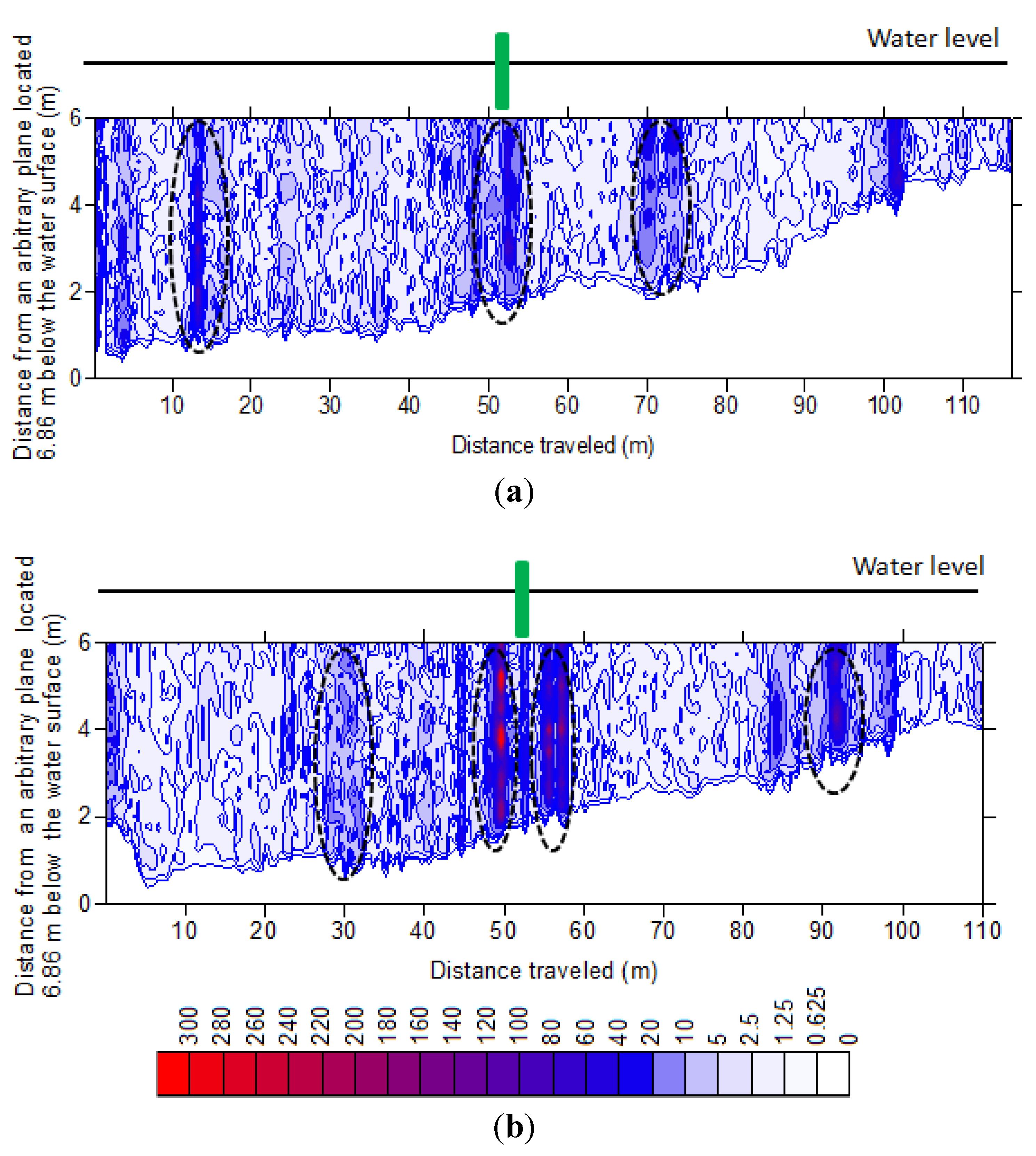
Figure 3 illustrates the vorticity magnitude, | | along the utmost downstream transects. Figure 3a corresponds to the DDD (minimum opening); Figure 3b shows the river condition when the DDD was not deployed (i.e., buoy only). Several zones of high vorticity values are clearly defined in the figure. Additionally, the graphs in the figure contain closed contours, which indicate the presence of vortexes [20].

Figure 3. Vorticity magnitude, | |, along the furthermost downstream transects. (a) DDD minimum opening; (b) buoy only. Dashed lines describe zones of high vorticity values. The scale is given in 1/s. Flow is going into the page. Projected DDD apex and buoy locations are indicated by green rectangles.

Figure 3. Vorticity magnitude, | |, along the furthermost downstream transects. (a) DDD minimum opening; (b) buoy only. Dashed lines describe zones of high vorticity values. The scale is given in 1/s. Flow is going into the page. Projected DDD apex and buoy locations are indicated by green rectangles.

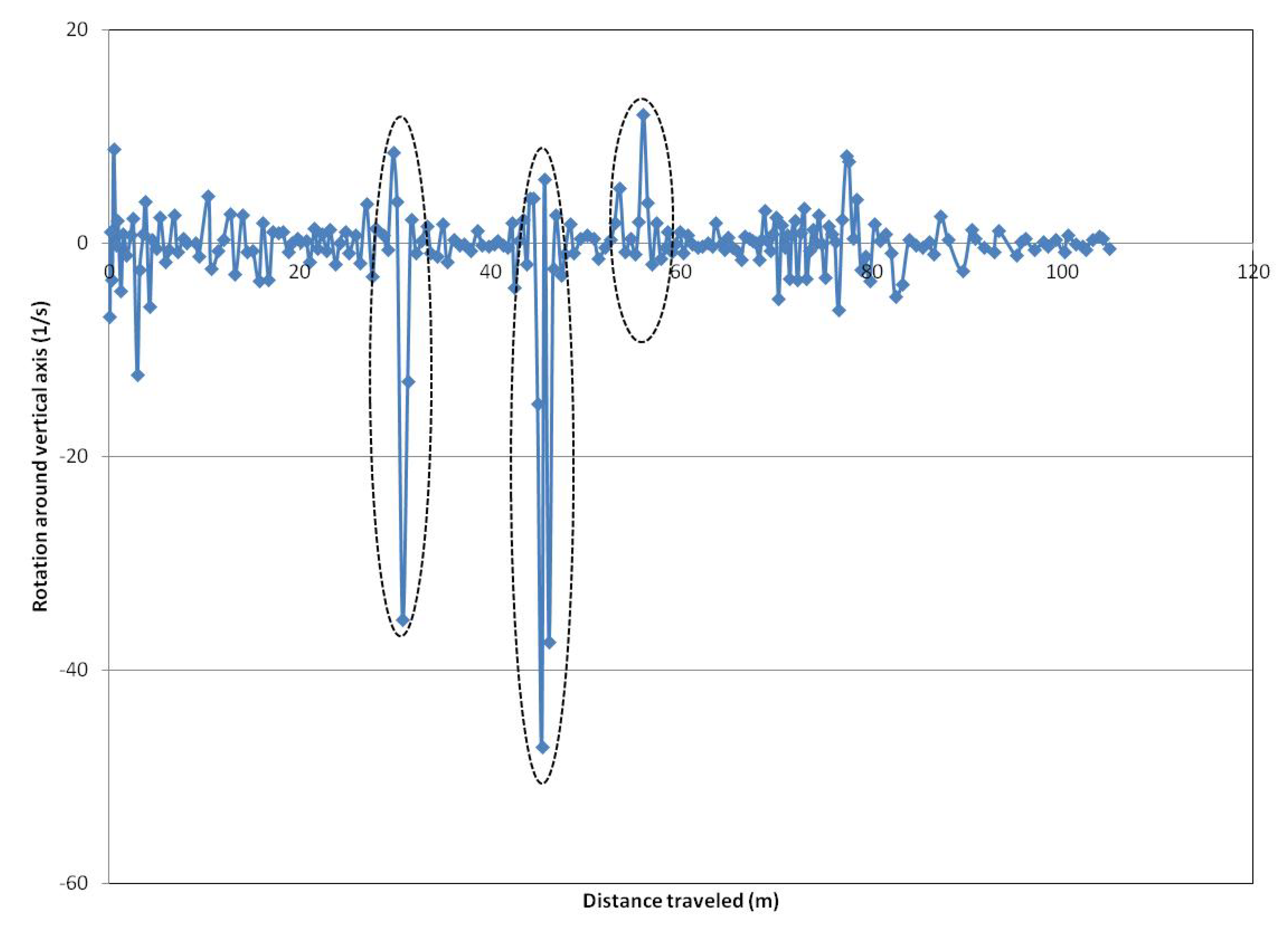
The graph in Figure 4 shows the angular rotation around the vertical axis for the transect located approximately 40 m downstream of the buoy (see Figure 2). Zones of high rotation values in both directions (i.e., positive and negative) are clearly identified in the graph. The background (or natural) river rotation values along the transect are at least one order of magnitude smaller than the rotation generated by the wakes created by the devices deployed in the river. The distance from the water surface for these plots is 1 m (center of the first bin). The graph indicates abrupt changes in the direction of rotation, which reflect the effects of the devices on flow conditions. Data reported in these figures were collected on 23 August 2012.

Figure 4. Rotation around the vertical axis along the transect located approximately 40 m downstream of the buoy. Dashed lines indicate zones of great changes. Projected DDD apex and buoy locations coincide with the zone of maximum change. Minimum DDD opening.

Figure 4. Rotation around the vertical axis along the transect located approximately 40 m downstream of the buoy. Dashed lines indicate zones of great changes. Projected DDD apex and buoy locations coincide with the zone of maximum change. Minimum DDD opening.

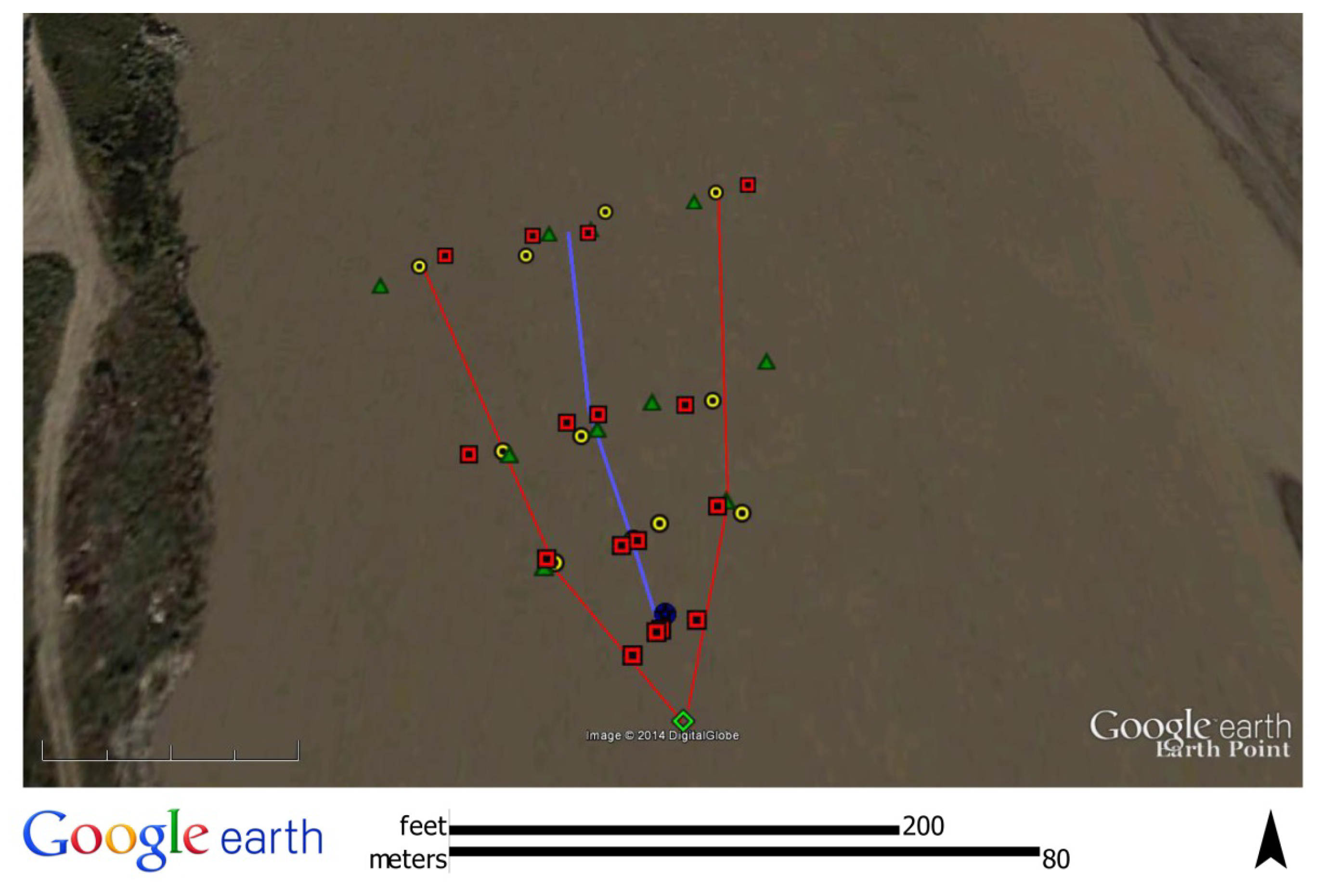
Specific locations in terms of latitude and longitude for all points with high rotation values were combined in a single figure (Figure 5). While some spread in the points is noticeable, in the downstream direction on both sides (left and right), the points indicate the extent of the wake generated by the buoy and/or DDD along the stream cross-sections. Points in the center show nearly consistent behavior (i.e., approximately the same location for a given transect, independent of the devices deployed in the stream). It is speculated here that these points illustrate the extended effects of the stud link chain deployed along the water column. Furthermore, the evidence of extended effects suggests that deployed hydrokinetic devices should not be centered behind a DDD, because significant flow rotation (see Figure 3 and Figure 4) and, consequently, extra turbulence are generated by the chain.

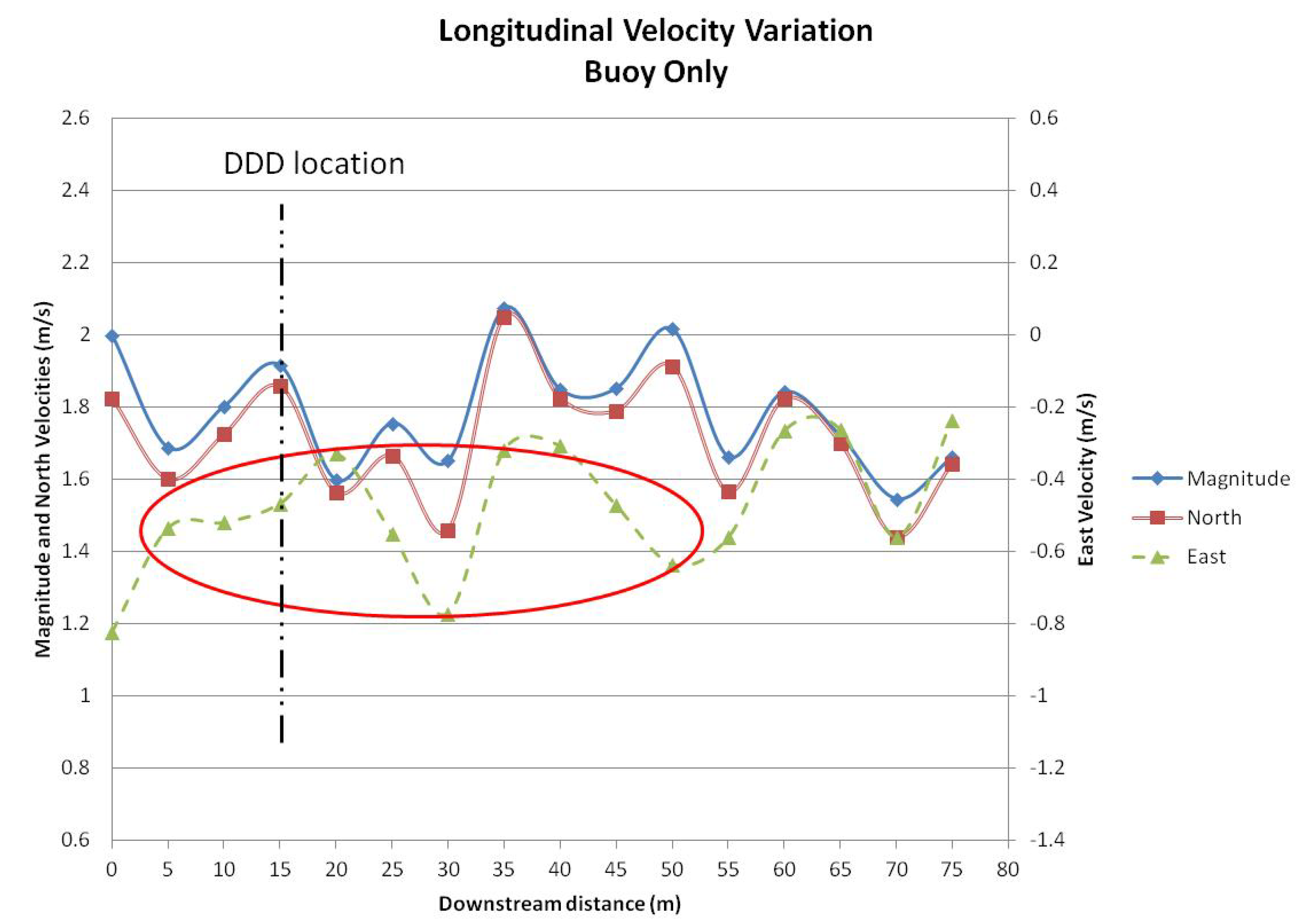
Graphs in Figure 6, Figure 7 and Figure 8 show the main flow characteristics (i.e., velocity magnitude and horizontal velocity components) for buoy only and minimum and maximum DDD openings, respectively. The figures point out that, as previously mentioned, the flow is predominantly in the north direction. In effect, velocity values in the north direction constitute at least 90% of the velocity magnitude, with the exception of the measurement closest to the devices (i.e., buoy and DDD).

Figure 5. Locations of significant rotation changes detected in all transects. Red squares indicate buoy only; green triangles denote DDD minimum opening; yellow circles show the DDD maximum opening. Lime squares and blue circles indicate buoy and DDD locations, respectively. Red and light blue lines indicate the average positions of the wakes. The flow direction is from bottom to top.

Figure 5. Locations of significant rotation changes detected in all transects. Red squares indicate buoy only; green triangles denote DDD minimum opening; yellow circles show the DDD maximum opening. Lime squares and blue circles indicate buoy and DDD locations, respectively. Red and light blue lines indicate the average positions of the wakes. The flow direction is from bottom to top.

Figure 6. The main flow characteristics along the longitudinal profile. Buoy only. The red oval shows a limited velocity variation in the east direction.

Figure 6. The main flow characteristics along the longitudinal profile. Buoy only. The red oval shows a limited velocity variation in the east direction.

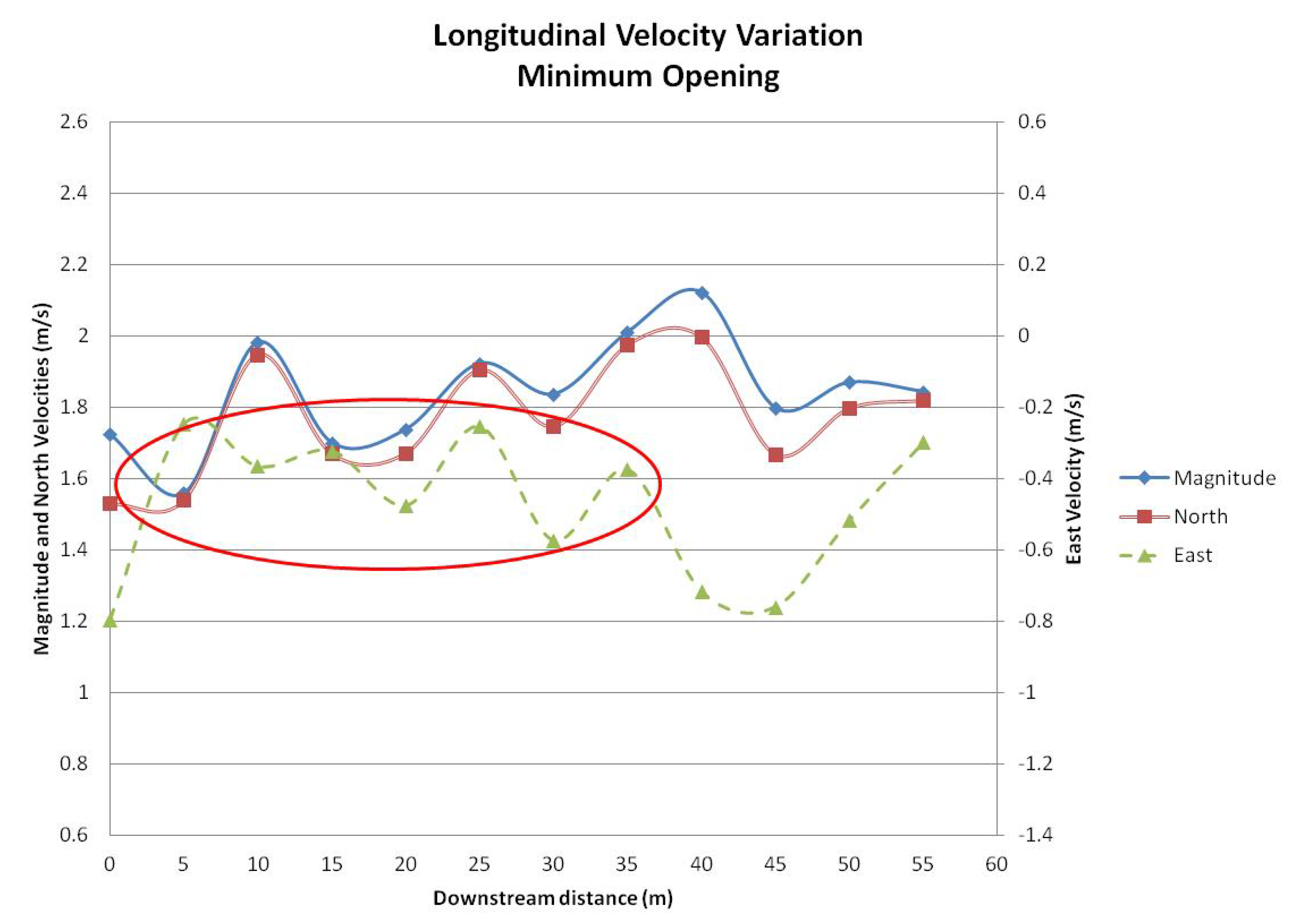
Figure 7. The main flow characteristics along the longitudinal profile. Minimum DDD opening. The red oval shows a limited velocity variation in the east direction.

Figure 7. The main flow characteristics along the longitudinal profile. Minimum DDD opening. The red oval shows a limited velocity variation in the east direction.

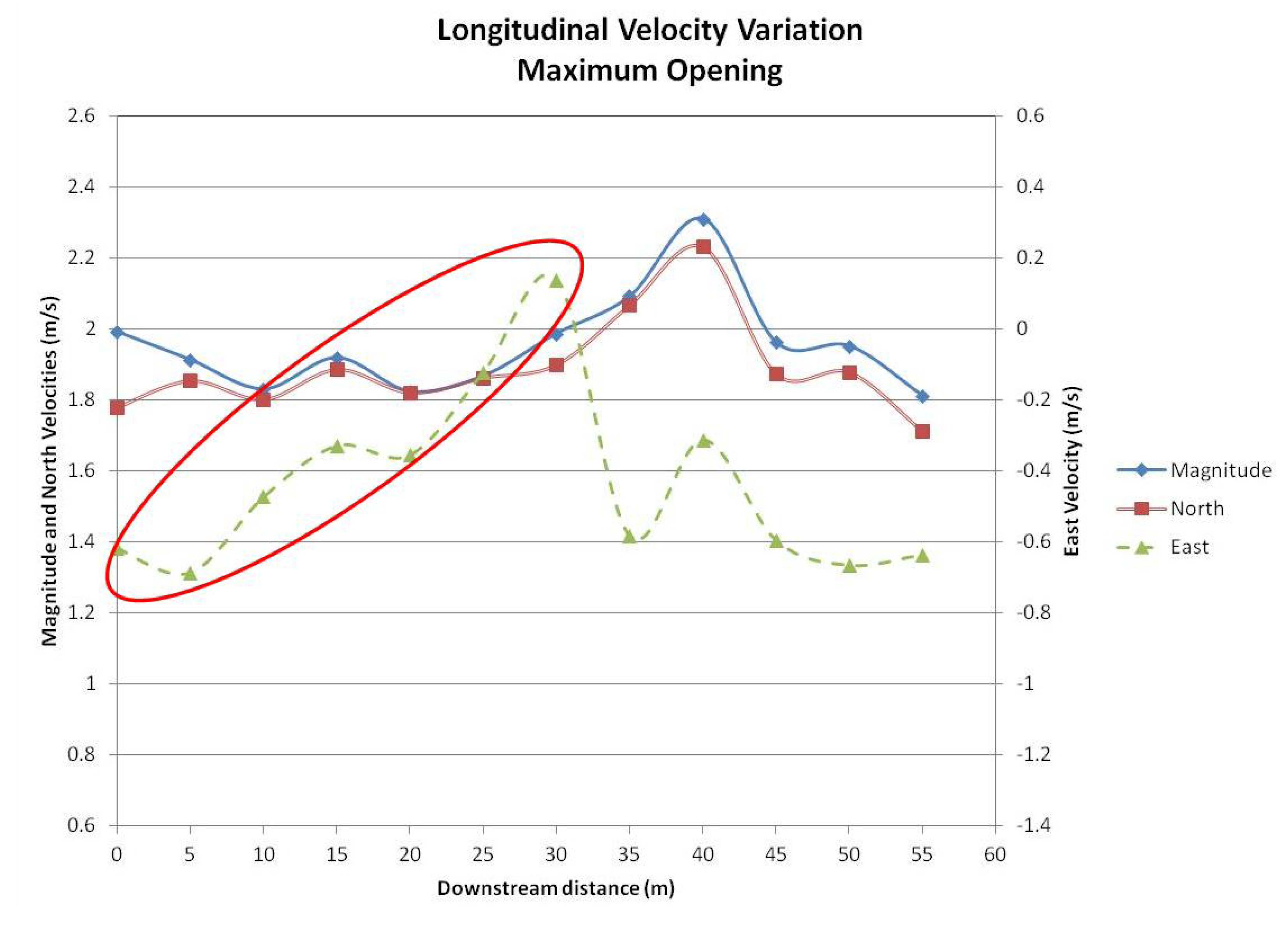
Figure 8. The main flow characteristics along the longitudinal profile. Maximum DDD opening. The red oval shows an important velocity variation in the east direction.

Figure 8. The main flow characteristics along the longitudinal profile. Maximum DDD opening. The red oval shows an important velocity variation in the east direction.

A comparison between the figures suggests noticeable changes in the east velocity direction and, consequently, high levels of macro-turbulence generated by the maximum opening (Figure 8). The velocity variation for the same direction in the cases of buoy only and minimum opening (Figure 6 and Figure 7) is somewhat limited, indicating a smaller signature in the flow. Based on the differences between velocity magnitude and velocity components, the plots indicate that vertical velocities are important in the vicinity of the buoy and DDD, which is another indication of high turbulence in that particular zone.

The available data indicate that flow in the streamwise direction (north) and, consequently, the velocity magnitude recover approximately 10–15 m downstream of the devices. This distance is roughly 2–3-times the water depth in the area. Thus, hydrokinetic turbines should be installed downstream of this zone.

While it is recognized that all data reported were collected by single river transects, the fact that areas of high rotation values were located approximately in the same spots for three different conditions (buoy only, minimum DDD opening and maximum DDD opening) shows the changes in river hydrodynamics, due to the devices (chain, buoy, and DDD) installed in the stream. The fact that areas of high rotation, which indirectly represents high turbulence, were detected along the projected buoy and DDD apex locations (Figure 5) indicates that large shear stresses should be expected there. Longitudinal profiles also provide insights on the changes in local velocities generated by the buoy and different DDD openings.

5. Conclusions

Two types of velocity measurements—cross-sectional velocity profiles and longitudinal velocity profiles—were conducted to identify changes in river hydrodynamics introduced by the installation of a DDD and associated devices (buoy and stud link chain).

Cross-sectional velocity measurements showed areas of high rotation values, which characterize the wakes generated by floating devices (buoy and DDD), as well as submerged elements (chain). Results indicate the strong effects on river hydrodynamics generated by the chain. These results should be of particular interest to project engineers, because they show that maximum velocity perturbations are located along the projection of the chain in the downstream direction.

Longitudinal velocity profiles show a reduction in velocity in the north direction and an increase in velocity along the west direction (immediately behind the DDD), indicating strong lateral flow conditions and, indirectly, high macro-turbulent conditions. Higher changes in lateral velocities were detected at the maximum opening.

Based on the results of this study, it is suggested that hydrokinetic turbines should not be installed, behind a surface DDD, at a distance smaller than 2–3-times the water depth. Additionally, high rotation should be expected along the projected buoy and DDD apex locations; this, in turn, could create unfavorable conditions for harvesting energy. Thus, it is recommended that hydrokinetic devices should not be deployed in the central area behind a surface DDD if a submerged chain is used to maintain the position of the DDD in the stream.