Attribution of Decadal-Scale Lake-Level Trends in the Michigan-Huron System

Abstract

This study disentangles causes of the Michigan-Huron system lake-level variability. Regional precipitation is identified as the primary driver of lake levels with sub-monthly time lag, implying that the lake-level time series can be used as a proxy for regional precipitation throughout most of the 1865–present instrumental record. Aside from secular variations associated with the Atlantic Multidecadal Oscillation, the lake-level time series is dominated by two near-decadal cycles with periods of 8 and 12 years. A combination of correlation analysis and compositing suggests that the 8-y cycle stems from changes in daily wintertime precipitation amounts associated with individual storms, possibly due to large-scale atmospheric flow anomalies that affect moisture availability. In contrast, the 12-y cycle is caused by changes in the number of instances, or frequency, of summertime convective precipitation due to a preferred upper-air trough pattern situated over the Great Lakes. In recent decades, the lake-level budget exhibited an abnormal—relative to the remainder of the instrumental record—evaporation-driven trend, likely connected to regional signatures of anthropogenic climate change. The latter effect must be accounted for, along with the effects of precipitation, when assessing possible scenarios of future lake-level variability.

1. Introduction

The Laurentian Great Lakes have over 10,000 miles of shoreline which is subject to submersion or drought depending on the water level of the lakes at any given time. Extremes in these levels affect shoreline erosion, cargo ship capacities, hydroelectric power supplies, and recreation for the basins’ inhabitants. While commonly considered two separate bodies of water, the second and third largest of the Great Lakes, Lake Michigan and Lake Huron, are connected by the deep Straits of Mackinac which ensures that the water levels of the separate reservoirs remain at equal elevations. Hence, they behave hydraulically like a single lake, and together, Lake Michigan-Huron has over 117,000 km² of surface water making it the world’s largest freshwater lake [1]. Given this vast surface area, it can reasonably be assumed that climate fluctuations should be well represented in the Michigan-Huron lake-level time series, and indeed several studies have indicated that precipitation is most likely the primary interannual lake-level driver [2,3,4,5,6]. Hence, in addition to addressing immediate socioeconomic impacts that the water levels have on surrounding communities, an understanding of the 1865–present lake-level time series also contributes to a better understanding of historic climate modes and regional precipitation behavior whose impacts extend to other area lakes and groundwater [7], river flows, and agriculture. While this extensive time series likely contains a great deal of information pertaining to past climate behavior, clear illustrations linking interannual lake-level fluctuations to regional precipitation variability have been lacking.

To better isolate climatic connections implicit in the lake-level time series, Hanrahan et al. [8] subtracted the outflow-related damping effects from the full lake-level record and determined that the resulting time series exhibits variability over a range of time scales. The longest time scale—secular variations are anti-correlated with North Atlantic sea-surface temperatures (SSTs). The climate mode associated with this SST signal has been dubbed the Atlantic Multidecadal Oscillation (AMO) and is associated with dynamics of the oceanic thermohaline circulation [9,10,11]. Previous studies have linked AMO phases to precipitation anomalies over large portions of the U.S. [12,13,14,15], and this signal is likely transmitted to the lake levels through precipitation changes [8]. In our previous work using Singular Spectrum Analysis (SSA: see Ghil et al. [16,17]), we also identified two near-decadal cycles in the Michigan-Huron water levels, namely the 8-y and 12-y cycles [6]. The latter signal is in agreement with Watras et al. [7] who identified a ~13-y cycle in lakes and aquifers across the upper Great Lakes’ region. The full lake-level time series can thus be decomposed as the sum of SSA reconstructed components associated with each decadal signal, and the residual variability is dominated by the AMO signal.

In this study, we aim to further our understanding of lake-level drivers responsible for decadal-scale lake-level changes. Using regional precipitation datasets, Section 2 establishes a solid connection between precipitation anomalies and lake-level variability, and addresses the issue of a possible time lag between precipitation forcing and lake-level response. In Section 3 and Section 4, we explore seasonality of near-decadal lake-level cycles and examine the large-scale atmospheric patterns associated with the corresponding lake-level changes. Section 5 summarizes our results on the connection between regional precipitation and historic lake-level changes, and addresses a recent evaporative trend which is becoming increasingly apparent in the previously precipitation-driven lake-level time series.

2. Michigan-Huron Lake-Level Drivers

The interannual Michigan-Huron lake levels fluctuate in response to the sum of five primary drivers (see Table 1 for a summary of variables used throughout the text): over-lake precipitation P_y, runoff from tributary rivers and streams R_y, evaporative losses −E_y, inflow through the St. Marys River from Lake Superior I_y, and outflow to the Mississippi River through the Chicago Diversion and the lower Great Lakes through the St. Clair River −O_y; the subscript y denotes the year under consideration. The estimated values for all these quantities were obtained online from the Great Lakes Environmental Research Laboratory (GLERL [18])).

Table 1. Descriptions of variables used throughout the text.

Variable	Description
Py	Annual total over-lake precipitation 1
Ry	Annual total runoff 1
Ey	Annual total evaporative losses 1
Iy	Annual total inflow (from Lake Superior for Lake Michigan-Huron) 1
Oy	Annual total outflow (through the St. Marys River and the Chicago Diversion for Lake Michigan-Huron) 1
$L_{m,y}^G$, $L_{m,y}^U$	Observed beginning-of-month lake-level as reported by GLERL (G) and monthly-average level by USACE (U)
dLm,y	Observed monthly lake-level change as estimated by Lm+1,y − Lm,y
$d{L}_y^s$, $d{L}_y^w$	Observed seasonal (3-month) lake-level change as estimated by dLm−1,y + dLm,y + dLm+1,y, where m = 7 for summer (s) and m = 12 for winter (w)
$d{L}_y^p$	Computed annual lake-level change associated with the precipitation-driven components 1 Py, Ry and Iy; see Equation (1)
$P_d^r$, $P_y^r$	Daily (d) and annual (y) total regional precipitation depth 2
$d{L}_y^{pr}$	Computed annual lake-level change associated with $P_y^r$; see Equation (2)
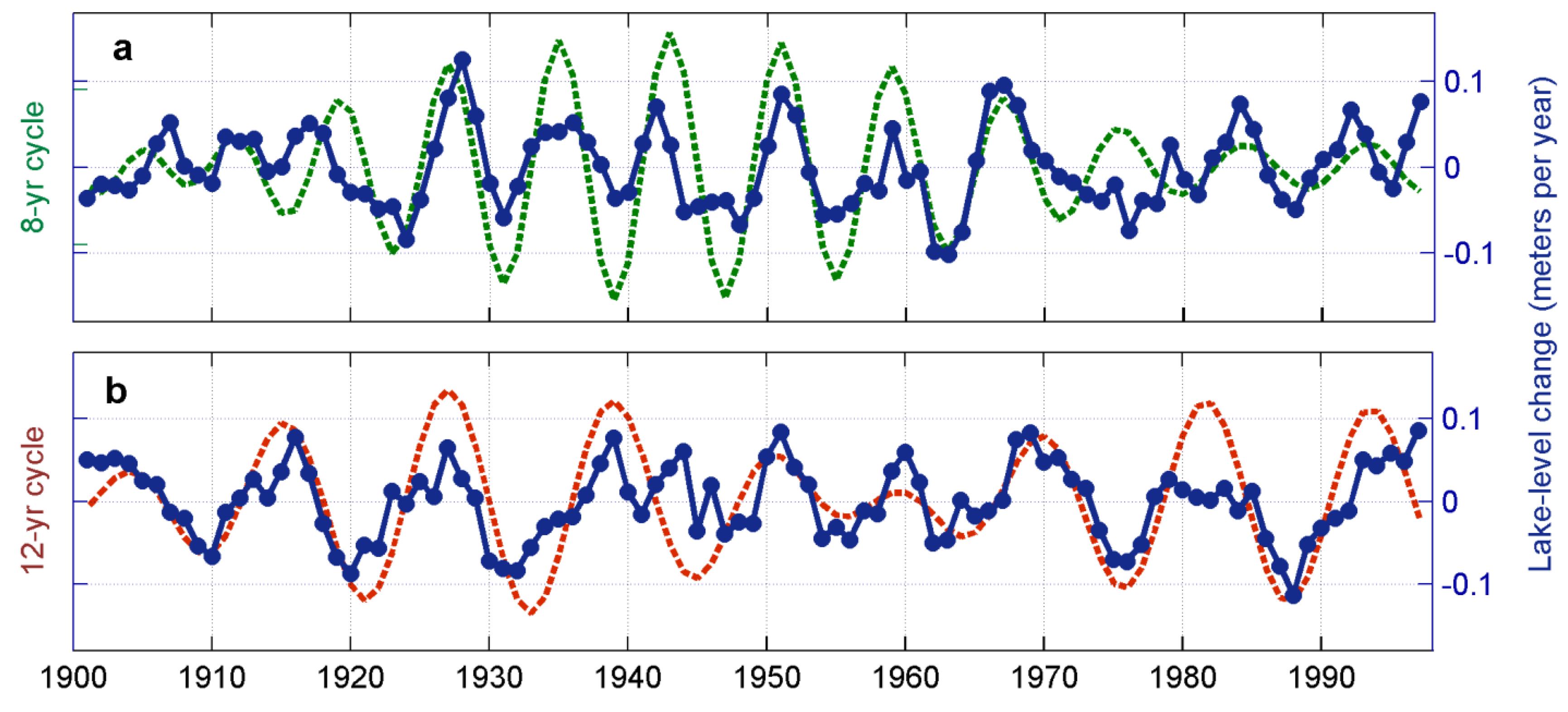
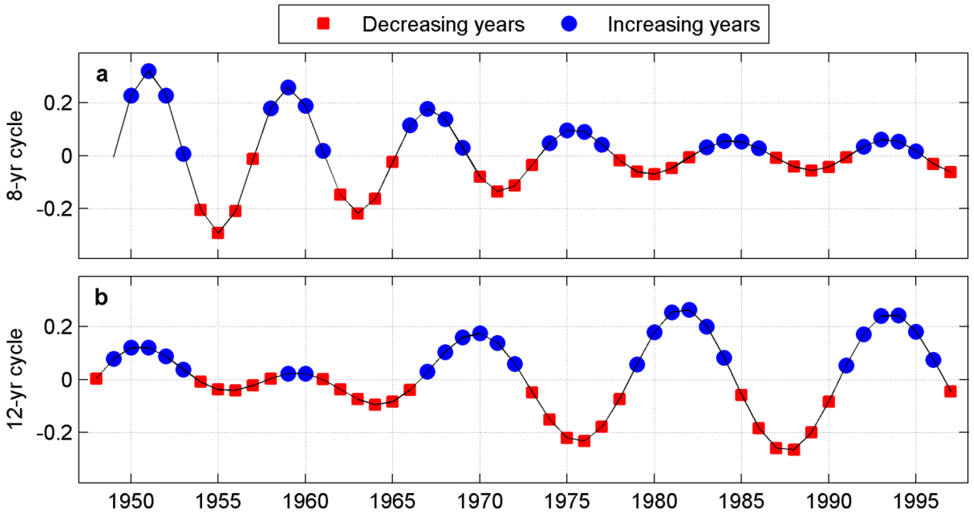
$L_y^{rc}$	Reconstructed lake-level components associated with the 8-y and 12-y cycles 3
$d{L}_y^{rc}$	Annual change of each reconstructed component as estimated by $L_{y+1}^{rc}$ − $L_{y-1}^{rc}$
PT	Average totaltotal precipitation 2 defined as
Pf	Average precipitation frequency 2, defined as
Pa	Average precipitation amount 2, defined as
${\hat{P}}^f$, ${\hat{P}}^a$	Precipitation frequency index ${\hat{P}}^f$, and amount ${\hat{P}}^a$, with multidecadal variability removed and averaged over 3 years

Notes: ¹ Lake fluxes are provided in linear units (depth) over the lakes surface from GLERL; ² Computed from the NOAA NCEP CPC gridded precipitation data; ³ Generated from statistically significant spectral peaks identified by Multi-taper method (MTM) analysis in Hanrahan et al. [6].

Table 1. Descriptions of variables used throughout the text.

Variable	Description
Py	Annual total over-lake precipitation 1
Ry	Annual total runoff 1
Ey	Annual total evaporative losses 1
Iy	Annual total inflow (from Lake Superior for Lake Michigan-Huron) 1
Oy	Annual total outflow (through the St. Marys River and the Chicago Diversion for Lake Michigan-Huron) 1
$L_{m,y}^G$, $L_{m,y}^U$	Observed beginning-of-month lake-level as reported by GLERL (G) and monthly-average level by USACE (U)
dLm,y	Observed monthly lake-level change as estimated by Lm+1,y − Lm,y
$d{L}_y^s$, $d{L}_y^w$	Observed seasonal (3-month) lake-level change as estimated by dLm−1,y + dLm,y + dLm+1,y, where m = 7 for summer (s) and m = 12 for winter (w)
$d{L}_y^p$	Computed annual lake-level change associated with the precipitation-driven components 1 Py, Ry and Iy; see Equation (1)
$P_d^r$, $P_y^r$	Daily (d) and annual (y) total regional precipitation depth 2
$d{L}_y^{pr}$	Computed annual lake-level change associated with $P_y^r$; see Equation (2)
$L_y^{rc}$	Reconstructed lake-level components associated with the 8-y and 12-y cycles 3
$d{L}_y^{rc}$	Annual change of each reconstructed component as estimated by $L_{y+1}^{rc}$ − $L_{y-1}^{rc}$
PT	Average totaltotal precipitation 2 defined as
Pf	Average precipitation frequency 2, defined as
Pa	Average precipitation amount 2, defined as
${\hat{P}}^f$, ${\hat{P}}^a$	Precipitation frequency index ${\hat{P}}^f$, and amount ${\hat{P}}^a$, with multidecadal variability removed and averaged over 3 years

Notes: ¹ Lake fluxes are provided in linear units (depth) over the lakes surface from GLERL; ² Computed from the NOAA NCEP CPC gridded precipitation data; ³ Generated from statistically significant spectral peaks identified by Multi-taper method (MTM) analysis in Hanrahan et al. [6].

2.1. Drivers of Lake-Level Changes

Three of the lake-level drivers—precipitation, runoff, and inflow—can all be tied to changes in regional precipitation. The over-lake precipitation, along with the river and stream flows that make up the runoff component, all stem from precipitation that occurs within the Michigan-Huron catchment basin. The inflow for Michigan-Huron has been regulated since 1887 by way of navigation locks on the St. Marys River to keep Lake Superior within a specified range of historic water levels [19]. If precipitation is the primary lake-level driver of Lake Superior, long-term precipitation variability over the Superior basin will thus be correlated with the regulated Michigan-Huron inflow.

The fourth lake-level driver, evaporation, is a major contributor to seasonal lake-level variability, but it has historically played a minor role in the behavior of the year-to-year lake level fluctuations. Between 1948 and 2005, annual evaporation totals exhibited a standard deviation of about 0.08 m, while the sum of the precipitation-driven components (precipitation, runoff, and inflow) had a standard deviation of 0.24 m over the same time period. Thus, the expected year-to-year lake-level changes stemming from evaporation variability are considerably smaller than those which occur from precipitation changes. The final lake-level driver, outflow, is a function of the lake-level itself and does not directly respond to atmospheric processes. It instead tends to damp the climate-related lake-level fluctuations arising from the four remaining components [8].

It follows that the historic annual lake-level changes can be largely described by the precipitation-driven components alone. The annual precipitation-driven lake-level changes $d{L}_y^p$ (Figure 1, black line) can thus be estimated as

$$d{L}_y^p=P_y+R_y+I_y-\stackrel{-}{E}-\stackrel{-}{O}$$

(1)

where P_y, R_y, and I_y values are all available for the period 1916–2005, while the historical averages of annual evaporative losses E, and the outflow average O are computed from 1948–2005 values.

Figure 1. Annual lake-level changes estimated from observed levels ($d{L}_y^U$; blue x’s) and as computed by Equation (1) ($d{L}_y^p$; black circles).

Figure 1. Annual lake-level changes estimated from observed levels ($d{L}_y^U$; blue x’s) and as computed by Equation (1) ($d{L}_y^p$; black circles).

The year-to-year lake-level variability associated with the precipitation-driven components alone (Figure 1; black line), as computed from Equation (1), accounts for about 87% (r = 0.93) of the 1916–2005 lake-level behavior as estimated from the monthly-averaged levels obtained from the U.S. Army Corps of Engineers (USACE) $d{L}_y^U$ (Figure 1; blue line). This indicates that precipitation has indeed had the greatest impact on interannual lake-level changes as it accounts for most of the historic lake-level variability. This precipitation–lake-level relationship is the primary focus of the present study.

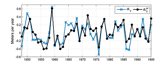
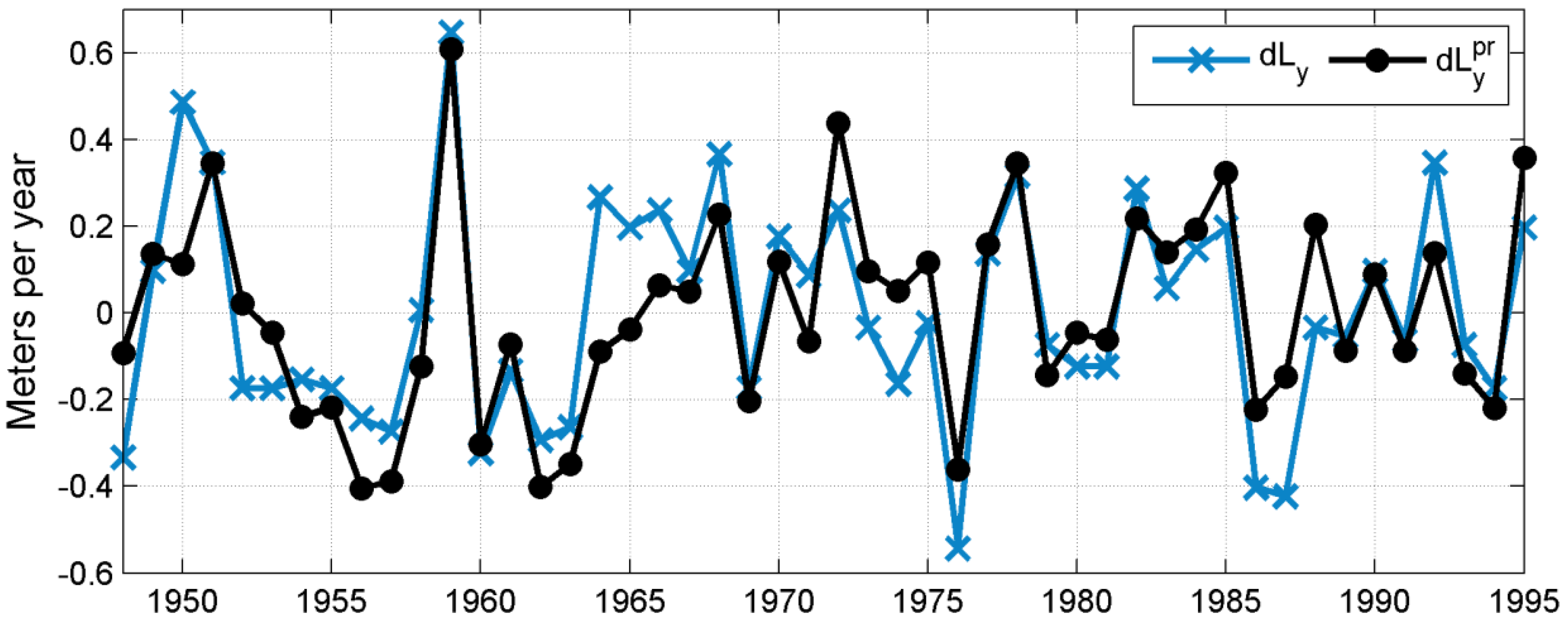
2.2. Connecting Regional Precipitation to Lake-Level Fluctuations

While the precipitation-driven components (precipitation, runoff, and inflow) alone can be used to describe much of the historic lake-level behavior, the determination of these individual values is still quite complex. For example, as discussed above, the inflow rates ultimately stem from annual precipitation over the Lake Superior basin, but there are additional factors that affect the amount of water that actually runs into Lake Michigan-Huron. Furthermore, because of ground absorption, evaporation, and other factors, the amount of precipitation that falls onto the land which surrounds Lake Michigan-Huron, is not equal to the amount of water that runs into the lake as runoff. Both the inflow and runoff as reported by GLERL must therefore be directly measured as they flow into the lake, or estimated by nearby flows. Here, we simplify the precipitation–lake-level connection by estimating these fluxes from precipitation indices alone.

We obtained NOAA NCEP Climate Prediction Center (CPC) daily precipitation data from the IRI/LDEO Climate Data Library [20]. This gridded data precipitation data product was based on raw data from NCDC daily co-op stations, the CPC dataset, and hourly precipitation datasets. The precipitation data for overlake gridpoints (Figure 2) were estimated from surrounding land-based stations via Cressman Scheme gridding onto a 0.25 degree grid. For the present analysis, seven of the resulting gridded locations over the Great Lakes’ basin were chosen as indicated by the red stars in Figure 2, for 1948–1997. Here, the over-Superior locations were selected to represent the Michigan-Huron inflow and the remaining locations represent the Michigan-Huron over-lake precipitation and runoff. Annual precipitation totals were computed from spatially averaged precipitation over the seven grid locations, resulting in a single 50-y time series of precipitation depths $P_y^r$. In order to estimate lake-level changes from these regional precipitation values, we must consider that the resulting Michigan-Huron lake-level variations are a multiple of $P_y^r$, because the surface area of Lakes Michigan and Huron makes up only a small fraction—about 1/5—of the total Michigan-Huron and Superior basin area A. For example, suppose that during a particular period there was an average rainfall of 3 mm in the region, and for simplicity, assume that all of it flowed directly into Lake Michigan-Huron. The total volume of water produced would be 3A mm³, which would equate to a lake-level increase of 3A × (1/5A)⁻¹ = 15mm, therefore amplifying the lake-level response by a factor of 5.

To compute lake-level changes given $P_y^r$, we used the historic instrumental record of individual precipitation-related components as reported by GLERL. Over the 1948–1997 time period, the average annual over-lake precipitation was P = 0.840 m, runoff R = 0.617 m, and inflow I = 0.604 m, while the average annual regional precipitation depth from the gridded dataset was $\stackrel{—}{P^r}$ = 0.697 m. The total annual Michigan-Huron over-lake precipitation, runoff, and inflow values, thus equate to about 2.96 times the regional precipitation depth. If this ratio remains relatively constant through our period of interest, lake-level change $d{L}_y^{pr}$ can be computed given only $P_y^r$, the historic average annual evaporative losses E = 0.64 m, and outflow O = 1.48 m (resulting in the subtraction of a constant value of 2.12 m). This results in the following simplified lake-level equation:

$$d{L}_y^{pr}=2.96P_y^r-2.12$$

(2)

The lake-level changes estimated from Equation (2) are illustrated in Figure 3 (black line) in conjunction with the observed lake-level change $d{L}_y^U$ (blue line). To account for possible delays related to snowpack storage, the annual rainfall totals illustrated here are defined with August as the beginning month.

Figure 2. Grid locations considered for regional precipitation estimate using NCEP CPC daily gridded precipitation data. Original image obtained from NOAA/GLERL.

Figure 2. Grid locations considered for regional precipitation estimate using NCEP CPC daily gridded precipitation data. Original image obtained from NOAA/GLERL.

Figure 3. Annual lake-level changes (July–August) estimated from observed levels ($d{L}_y^U$; blue x’s) and as computed by Equation (2) ($d{L}_y^{pr}$; black circles).

Figure 3. Annual lake-level changes (July–August) estimated from observed levels ($d{L}_y^U$; blue x’s) and as computed by Equation (2) ($d{L}_y^{pr}$; black circles).

While numerous difficult-to-measure processes are occurring which affect the lake-level water supply (i.e., over-lake and river evaporation, over-land evaporation, channel adjustments, vegetative consumption, groundwater intake, among several others), this simplified regional precipitation index $d{L}_y^{pr}$ still accounts for the majority of lake-level variability (r = 0.81). This ability to connect the lake-level changes directly to a single atmospheric variable is ideal for furthering our understanding of underlying atmospheric behavior. In particular, one can use the lake-level time series, which begins at 1865, and Equation (2) to estimate regional precipitation prior to 1948, where the CPC gridded precipitation dataset is not available, thus providing a much extended period during which to study rainfall variability.

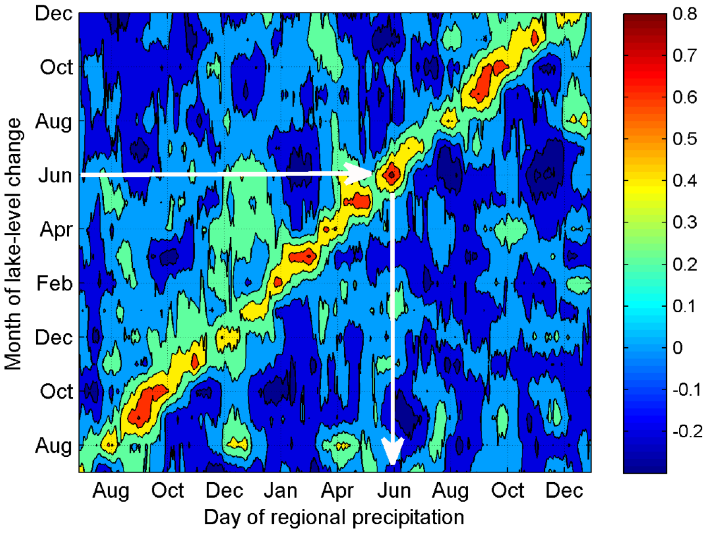
2.3. Lag Time of Precipitation Effects on Lake-Level Changes

To investigate the possibility of a sub-annual time lag between precipitation and lake-level changes, we compared monthly lake-level changes estimated from beginning-of-month lake level data provided by GLERL $d{L}_{m,y}^G$ to 30-day precipitation totals $P_d^r$. Correlation coefficients were computed between the 50-year-long monthly time series of $d{L}_{m,y}^G$ and daily time series of $P_d^r$. To account for potential end-of-year water-level lag times, the years were overlapped, so that correlations were computed for all months and days July 1948–December 1949 to July 1996–December 1997. The contour plot in Figure 4 illustrates the magnitude of these correlations where months along the horizontal axis refer to the first day of 30-day precipitation totals $P_d^r$, and those along the vertical axis indicate the month of lake-level change $d{L}_{m,y}^G$. For example, the lake-level changes in June (from left axis), correlate most strongly with the 30-day precipitation totals that begin on about June 1 of the same year (bottom axis), where r ≈ 0.8; the points that correspond to this example are indicated by the white arrows. On average, statistically significant correlations (p < 0.5) occur where r > 0.45. Because the strongest correlations occur during concurrent times, we conclude that the lake levels primarily respond to regional precipitation with a sub-monthly time lag. Therefore, any season-specific variability in the water levels of Michigan-Huron should agree with the timing of regional precipitation drivers.

Figure 4. Correlations between regional precipitation $P_d^r$ that begin on the dates along the horizontal axis, and monthly lake-level changes $d{L}_{m,y}^G$ that occur during the months along the vertical axis. The shading indicates the strength of correlation (r), as indicate by the bar on the right. The average r-values which significantly exceed zero are 0.45 (p < 0.05) and 0.55 (p < 0.01). See text for further explanation.

Figure 4. Correlations between regional precipitation $P_d^r$ that begin on the dates along the horizontal axis, and monthly lake-level changes $d{L}_{m,y}^G$ that occur during the months along the vertical axis. The shading indicates the strength of correlation (r), as indicate by the bar on the right. The average r-values which significantly exceed zero are 0.45 (p < 0.05) and 0.55 (p < 0.01). See text for further explanation.

3. Timing of Lake-Level Changes and Precipitation Behavior

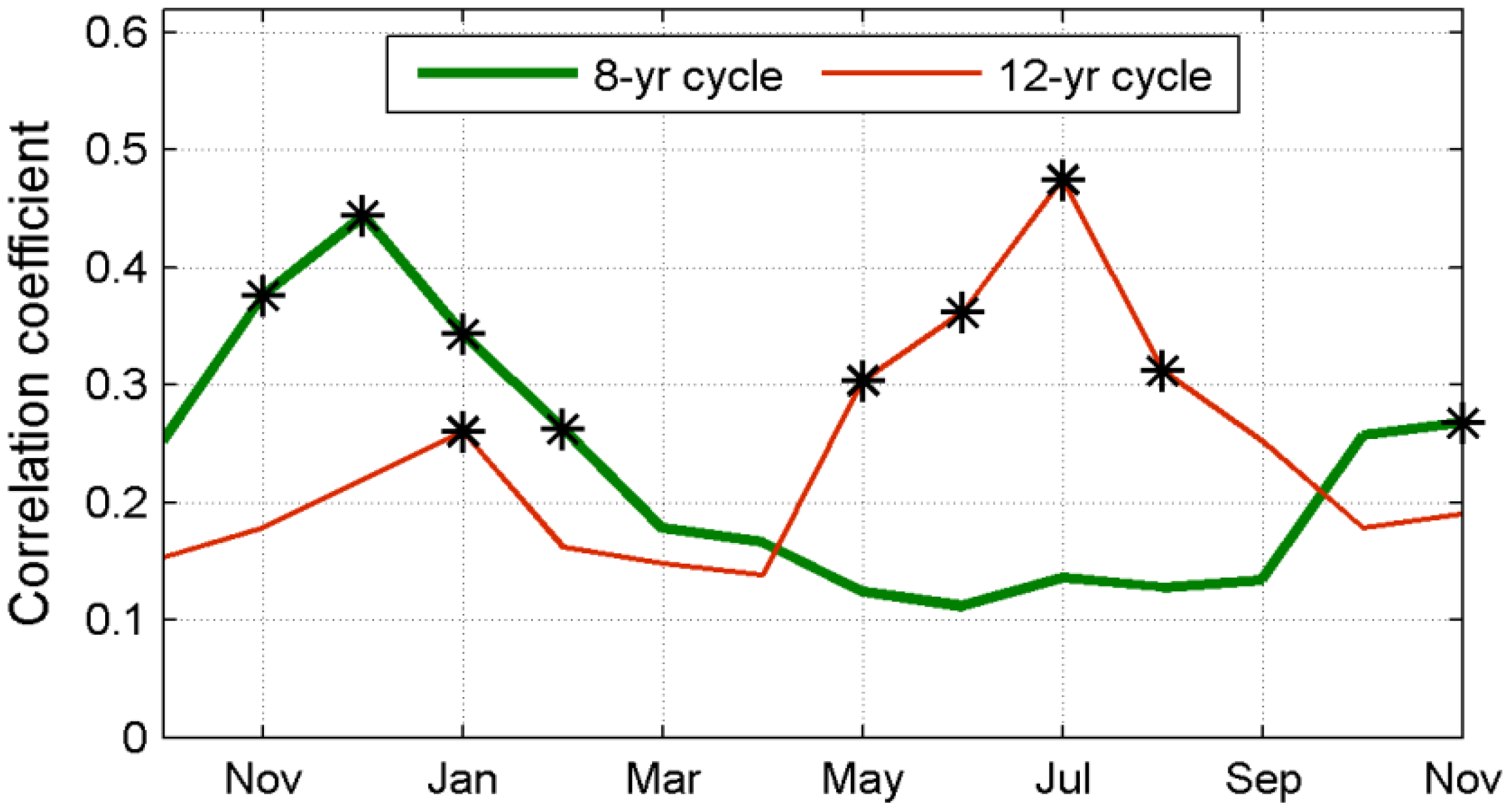
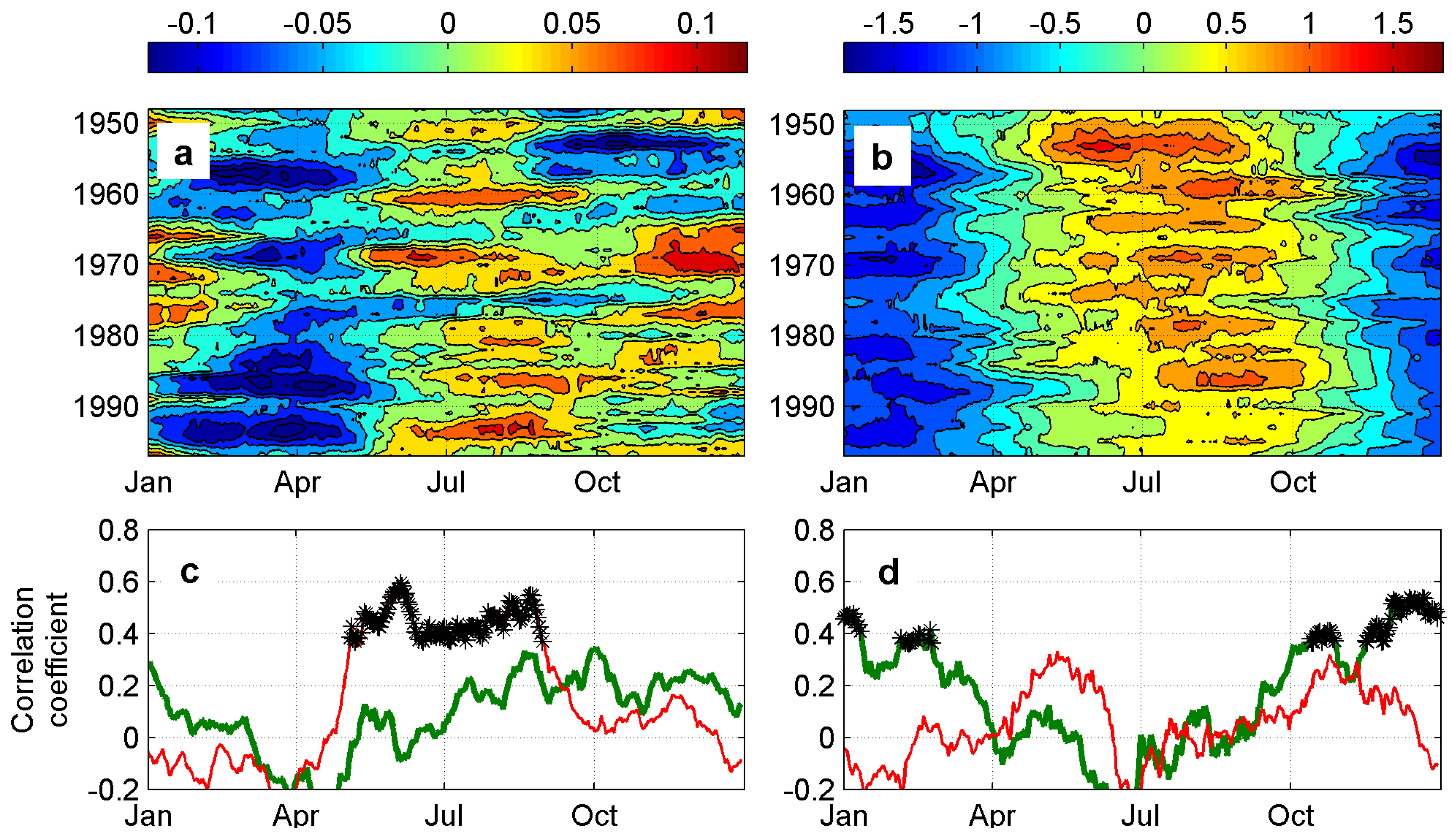
3.1. Seasonality of Lake-Level Periodicities

We now investigate potential seasonality in lake-level quasi-periodicities previously identified in Hanrahan et al. [6]. For this analysis, seasonal (3-month) lake-level changes $d{L}_{m,y}^G$ were compared to the derivatives $d{L}_y^{rc8}$ and $d{L}_y^{rc12}$ of the reconstructed lake-level components corresponding to the 8-y and 12-y signals identified by the SSA analysis of the 1865–1999 lake-level time series; see Hanrahan et al. [6], and Ghil et al. [16,17] for details pertaining to the computation of reconstructed components. Correlations between 24 consecutive months of lake-level changes $d{L}_{m,y}^G$ and the reconstructions $d{L}_y^{rc}$ are illustrated in Figure 5 for the lake-level change periods of October 1900–1998 to November 1901–1999. For example, the first November correlations (left) are between the November 1900–1998 lake-level changes and the 1901–1999 reconstructions, $d{L}_y^{rc8}$ (thick green) and $d{L}_y^{rc12}$ (thin red), respectively. The second November correlations (right) are between the same reconstruction years, and the November 1901–1999 lake-level changes. Because artificially-high correlations may be generated among time series exhibiting red-noise variability, a Monte Carlo test was used to establish significance of the co-variance between the reconstructions and seasonal lake-level behavior by generating 1000 surrogate lake-level time series using the same length and lag-1 autocorrelation as the actual lake-levels. Correlations were computed between the surrogate time series and the reconstructions, which were sorted and then compared to the observed values. The observed values exceeding the 99th percentile of the synthetic values were determined to be significant at the 1% level (black stars in Figure 5).

Figure 5. Correlation between the 8-y ($d{L}_y^{rc8}$; thick green) and 12-y ($d{L}_y^{rc12}$; thin red) reconstructed lake-level changes, and the observed seasonal (3-month) lake-level changes ($d{L}_{m,y}^G$). Black stars indicate correlations significant at the 1% level.

Figure 5. Correlation between the 8-y ($d{L}_y^{rc8}$; thick green) and 12-y ($d{L}_y^{rc12}$; thin red) reconstructed lake-level changes, and the observed seasonal (3-month) lake-level changes ($d{L}_{m,y}^G$). Black stars indicate correlations significant at the 1% level.

The 8-y reconstruction best correlates with lake-level changes during the preceding winter months of November to January. Conversely, the 12-y cycle is dominant during the summer months, as the peak correlations occur during June to August. The smoothed (3-y average) lake-level change time series that correspond to these seasons (blue) are illustrated in Figure 6a for the winter months $d{L}_y^w$ (November–January) and Figure 6b for the summer months $d{L}_y^s$ (June–August), along with the derivatives $d{L}_y^{rc}$ of the 8-y and 12-y cycles (Figure 6a,b, green and red dashed lines, respectively). We have thus established that the two near-decadal lake-level periodicities occur during different times of the year; the 8-y cycle during winter months, and the 12-y cycle during summer months.

Figure 6. (a) Detrended wintertime (November–January) lake-level changes $d{L}_y^w$ (blue) and the derivative of the 8-y lake-level reconstruction $d{L}_y^{rc8}$ (green dashed); (b) Detrended summertime (June–August) lake-level changes $d{L}_y^s$ (blue) and the derivative of the 12-y lake-level reconstruction $d{L}_y^{rc12}$ (red dashed).

Figure 6. (a) Detrended wintertime (November–January) lake-level changes $d{L}_y^w$ (blue) and the derivative of the 8-y lake-level reconstruction $d{L}_y^{rc8}$ (green dashed); (b) Detrended summertime (June–August) lake-level changes $d{L}_y^s$ (blue) and the derivative of the 12-y lake-level reconstruction $d{L}_y^{rc12}$ (red dashed).

3.2. Seasonality of Precipitation Characteristics

Because regional precipitation drives lake-level changes with sub-monthly time lag (Section 2.3), it follows that the lake-level cycle seasonalities identified above (Section 3.1) should coincide temporally with those of precipitation. In this section, we examine potential seasonal precipitation periodicities by comparing the reconstructed lake-level cycles to two precipitation indices: frequency and amount. Both indices were computed from the daily gridded CPC precipitation data and are defined as follows:

(3)

(4)

where a “precipitation day” is defined as having measurable precipitation (at least 1 mm) in one or more of the seven grid locations, and the sum of precipitation is computed as the average precipitation depth over all grid locations summed up over a specified number of days. Hence, P^f indicates the probability of precipitation occurring on any given day, irrespective of the intensity of the precipitation-producing system. Conversely, P^a is related to the intensity of precipitation during individual storm events, as it accounts for the average amount of precipitation that fell during a given precipitation day and location, not for the number of instances or spatial extent. These metrics are similar to those used by other authors where daily “frequency” and “amount” are sometimes referred to as “relative number of wet days” and “intensity,” respectively [21].

To encompass full seasons, P^f and P^a were computed over 120-day moving segments (total number of days = 120) over 1948–1997. As identified in Hanrahan [22], both of these indices exhibit significant multidecadal variability possibly associated with the AMO. To filter out this low-frequency variability, we subtracted 20-y moving averages from both indices. Next, to minimize the highest-frequency variability for the purpose of concentrating on decadal time scales, we computed 3-y moving averages of the final time series. The resulting filtered indices ${\hat{P}}^f$ and ${\hat{P}}^a$ are illustrated in Figure 7a,b, respectively.

To evaluate the existence of near-decadal cycles in precipitation frequency and amount, correlation coefficients were computed between the two indices and the reconstructed derivatives. That is, 365 50-year-long time series of ${\hat{P}}^f$ and ${\hat{P}}^a$ (vertical axes in Figure 7a,b) which correspond to each day of the year (defined in months on the horizontal axes), were compared to each 50-year-long time series of the 8-y and 12-y reconstructed derivatives, $d{L}_y^{rc8}$ and $d{L}_y^{rc12}$. Precipitation frequency ${\hat{P}}^f$ best correlates with the 12-y cycle during the summer months (Figure 7c, thin red; black stars indicate correlations significant at the 1% level), and the precipitation amount index ${\hat{P}}^a$ correlates best with the 8-y cycle during the winter months (Figure 7d, thick green). These results are consistent with the previously-discussed timing of periodicities, where the 12-y and 8-y cycles were linked to the summertime and wintertime lake-level changes, respectively (Section 3.1).

Figure 7. Identification of precipitation characteristics associated with the 8-y and 12-y lake-level cycles. Filtered 120-day moving averages of regional precipitation (a) frequency ${\hat{P}}^f$ and (b) amount ${\hat{P}}^a$; (c,d) Correlations between the precipitation indices (from a and b) and the 8-y cycle $d{L}_y^{rc8}$ (thick green lines) and 12-y cycle $d{L}_y^{rc12}$ (thin red lines). Black stars indicate significant correlations at 1% level.

Figure 7. Identification of precipitation characteristics associated with the 8-y and 12-y lake-level cycles. Filtered 120-day moving averages of regional precipitation (a) frequency ${\hat{P}}^f$ and (b) amount ${\hat{P}}^a$; (c,d) Correlations between the precipitation indices (from a and b) and the 8-y cycle $d{L}_y^{rc8}$ (thick green lines) and 12-y cycle $d{L}_y^{rc12}$ (thin red lines). Black stars indicate significant correlations at 1% level.

3.3. Verification of Seasonal Characteristics

To further establish significance of these findings, we compared monthly precipitation indices from Equations (3) and (4) during opposing phases of the 8-y and 12-y cycles. The 1948–1997 reconstruction derivatives $d{L}_y^{rc}$ were divided into two categories: increasing and decreasing lake-level years, as illustrated in Figure 8 (blue circles and red squares, respectively). For the 12-y periodicity (Figure 8b, black line), summertime (June–August) monthly precipitation indices were categorized during 1948–1997, resulting in 25 years, or 75 individual months, per phase. For the 8-y periodicity (Figure 8a, black line), wintertime (September–January) indices were categorized during 1949–1997 (the 1948 winter was not included because November–December data were not available for 1947), resulting in 24 years, or 72 months, per phase.

Figure 8. (a) Derivatives of 8-y lake-level reconstruction $d{L}_y^{rc8}$ and (b) the 12-y reconstruction $d{L}_y^{rc12}$ (black lines), and categorization of phases: increasing lake-level years (blue circles) and decreasing lake-level years (red squares).

Figure 8. (a) Derivatives of 8-y lake-level reconstruction $d{L}_y^{rc8}$ and (b) the 12-y reconstruction $d{L}_y^{rc12}$ (black lines), and categorization of phases: increasing lake-level years (blue circles) and decreasing lake-level years (red squares).

In addition to the precipitation frequency P^f and amount P^a indices, we have also included a total precipitation index P^T, for comparison. This index was defined as the total precipitation amount over the total number of days under consideration:

(5)

where the denominator includes all days, both precipitating and non-precipitating. When summed up over a month, P^T amounts to the expected total area-averaged precipitation, which can be translated to monthly lake-level changes with Equation (2). On the other hand, the precipitation frequency index P^f, which represents the probability of precipitation occurring during any given day through the month, results in the number of days with some amount of precipitation within the Superior/Michigan-Huron region. The precipitation amount index P^a represents the average daily precipitation amount only during precipitation days.

We computed each index value during years of increasing and decreasing lake levels, over winter ($P_w^T$, $P_w^f$, $P_w^a$) and summer ($P_s^T$, $P_s^f$, $P_s^a$) months. The means were tested for significant differences with a one-sided t-test, between the phases of the 8-y cycle (Table 2) and the 12-y cycle (Table 3). We find that P^T is significantly different between the phases of both periodicities—$P_w^T$ during the 8-y cycle, and $P_s^T$ during the 12-y cycle—indicating that more precipitation fell during the increasing phases of these periodicities than during the decreasing phases. This is in agreement with our results from Section 3.1 that compared seasonal lake-level changes to the lake-level reconstructions. Furthermore, the wintertime precipitation amount index $P_w^a$ is significantly different between the phases of the 8-y cycle, and the summertime precipitation frequency index $P_s^f$ is significantly different between phases of the 12-y cycle. This is in agreement with our findings from Section 3.2 that examined correlations between rainfall indices and lake-level reconstructions.

Table 2. Precipitation indices during winter months associated with the increasing and decreasing phases of the 8-y cycle*.

Index	Average	Increasing	Decreasing	Significance
Total precipitation $P_w^T$ (daily average in mm)	1.58	1.67	1.49	p = 0.03
Frequency $P_w^f$ (daily probability)	0.72	0.73	0.72	p = 0.44
Amount $P_w^a$ (daily average in mm)	2.18	2.29	2.06	p = 0.01

Note: * p-values in bold indicate significant differences between the increasing and decreasing phases of the 8-y cycle as determined by a one-sided t-test (p < 0.05).

Table 2. Precipitation indices during winter months associated with the increasing and decreasing phases of the 8-y cycle*.

Index	Average	Increasing	Decreasing	Significance
Total precipitation $P_w^T$ (daily average in mm)	1.58	1.67	1.49	p = 0.03
Frequency $P_w^f$ (daily probability)	0.72	0.73	0.72	p = 0.44
Amount $P_w^a$ (daily average in mm)	2.18	2.29	2.06	p = 0.01

Note: * p-values in bold indicate significant differences between the increasing and decreasing phases of the 8-y cycle as determined by a one-sided t-test (p < 0.05).

Table 3. Precipitation indices during summer months associated with the increasing and decreasing phases of the 12-y cycle*.

Index	Average	Increasing	Decreasing	Significance
Total precipitation $P_s^T$ (daily average in mm)	2.38	2.50	2.26	p = 0.02
Frequency $P_s^f$ (daily probability)	0.72	0.75	0.70	p < 0.01
Amount $P_s^a$ (daily average in mm)	3.26	3.32	3.20	p = 0.20

Note: * p-values in bold indicate significant differences between the increasing and decreasing phases of the 12-y cycle as determined by a one-sided t-test (p < 0.05).

Table 3. Precipitation indices during summer months associated with the increasing and decreasing phases of the 12-y cycle*.

Index	Average	Increasing	Decreasing	Significance
Total precipitation $P_s^T$ (daily average in mm)	2.38	2.50	2.26	p = 0.02
Frequency $P_s^f$ (daily probability)	0.72	0.75	0.70	p < 0.01
Amount $P_s^a$ (daily average in mm)	3.26	3.32	3.20	p = 0.20

Note: * p-values in bold indicate significant differences between the increasing and decreasing phases of the 12-y cycle as determined by a one-sided t-test (p < 0.05).

In summary, it is changes in seasonal precipitation totals P^T that are driving the near-decadal lake-level cycles, and these totals vary due to changes both in precipitation frequency P^f and precipitation amount P^a. Consistent with our findings discussed in the previous section, we conclude that precipitation fluctuations associated with the 8-y wintertime cycle are largely stemming from changes in precipitation amounts during the winter months $P_w^a$. Conversely, the summertime 12-y cycle is primarily being driven by changes in precipitation fluctuations through variations in summertime precipitation frequency $P_s^f$.

4. Climate Connections

To identify large-scale climate variability associated with the cyclic Michigan-Huron lake-level changes, we compared the winter and summer time series of lake-level tendencies $d{L}_y^w$ and $d{L}_y^s$ (Figure 6, blue lines) to the evolution of various atmospheric fields and SSTs. We hypothesize that the actual lake-level changes serve as a more accurate proxy for seasonal precipitation totals due to the spatial restrictions and coarse temporal resolution of the actual precipitation data.

We used monthly averaged 1949–1998 NOAA NCEP-NCAR reanalysis data for 850-mb air temperatures, sea-level pressures (SLPs), and 500-mb geopotential heights, and Kaplan et al. [23] gridded SSTs analyzed over the same time period. The climatological monthly means were removed from all indices, and 20-y moving averages were subtracted from each location’s time series to concentrate on decadal scales. The anomalous lake-level changes, $d{L}_y^w$ and $d{L}_y^s$, were sorted into years from the largest negative to the largest positive lake-level change, and the first and last 12 years—approximately the upper and lower 25% of all available years—were selected. Next, we generated composite plots to connect the behavior of seasonal lake-level fluctuations to atmospheric and SST variability. The differences between the composites over the years with the greatest positive and negative lake-level changes during winter $d{L}_y^w$ and summer $d{L}_y^s$, are illustrated in Figure 9 and Figure 12, respectively, where $d{L}_y^w$ was compared to November–January, and $d{L}_y^s$ was compared to June–August anomalies of SSTs (°C), SLPs (mb), 850-mb air temperatures (°C), and 500-mb heights (m). The white lines encompass areas where the upper and lower means were determined to be significantly different at the 5% confidence level, as determined by a two-sided t-test.

4.1. The 8-y Wintertime Cycle

We concluded in Section 3 that the 8-y lake-level cycle is active during November–January, and found variations in wintertime precipitation amounts $P_w^a$ to be the primary driver. Hence, atmospheric connections to Michigan-Huron lake-level changes during these months can help to identify climate modes associated with this periodicity.

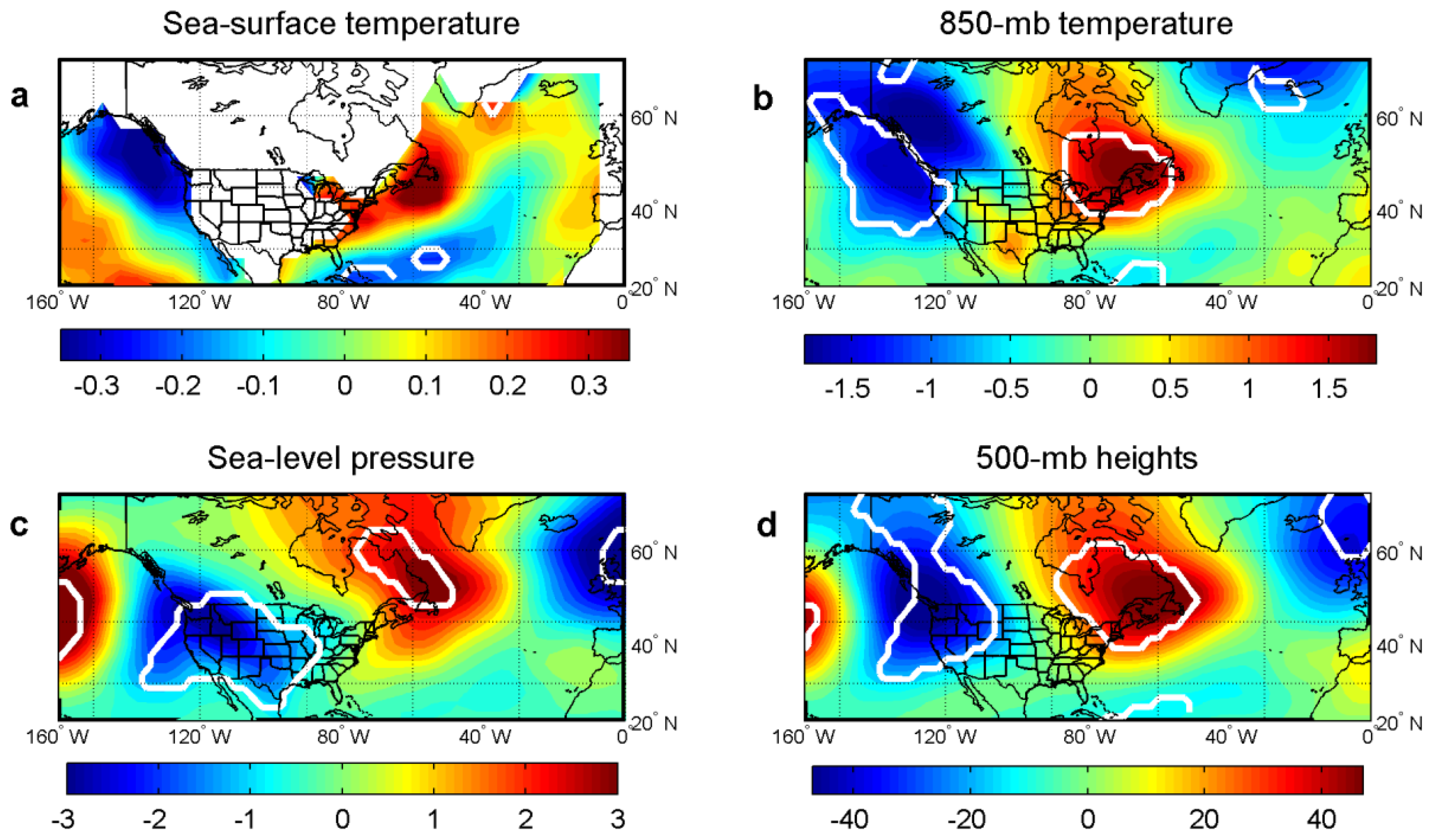
4.1.1. Wintertime Anomalies

Composite North Atlantic and North Pacific SST anomalies (Figure 9a) associated with the wintertime lake-level changes $d{L}_y^w$ have patterns similar to those of the 850-mb temperatures (Figure 9b) and upper-level heights (Figure 9d). The years of greatest wintertime lake-level increase correspond to a warm North Atlantic SST anomaly off the New England coast, which underlies a positive 850-mb temperature and 500-mb height anomaly, both extending back over part of the Great Lakes’ region. Also during these years, below-average 850-mb temperatures and 500-mb heights are observed along the northwestern edge of the U.S. and western Canada. These climate patterns are characteristic of an increased precipitation-producing storm-track displacement, where the trough over the western U.S. indicates a southward displacement, and the ridge over northeastern U.S. indicates a northward displacement. Hence, it appears that wintertime cyclones that travel over the U.S. during increasing lake-level years tend to be of more southern origin, allowing more moisture from the Gulf of Mexico to reach the Great Lakes’ region. Another way to interpret moisture transport is by examination of the SLP plot (Figure 9c). The anomalous cyclonic rotation of the low SLPs in the southwest (Colorado low), combined with the anomalous anticyclonic rotation of the anomalous high SLPs in the northeast, set up an anomalous northeastward flow (Panhandle hook) directly transporting moisture from the Gulf of Mexico toward the Great Lakes, resulting in greater precipitation amounts there.

We additionally examined potential differences in precipitable water (kg/m²) associated with storm-track displacements (Figure 10; analogous to composite plots of Figure 9). A statistically significant positive anomaly in precipitable water includes most of the Great Lakes’ region and is consistent with that which would be expected from a northward storm track displacement over the eastern U.S, further substantiating our findings that the wintertime lake-level changes are associated with moisture anomalies stemming from variations in storm track.

Figure 9. Composite differences between the 12 years with the greatest increase and 12 years with the greatest decrease of wintertime (NDJ) lake-level, for high-pass filtered seasonal anomalies of (a) SSTs; (b) 850-mb temperatures; (c) SLPs; and (d) 500-mb geopotential heights, for 1949–1998. Areas encompassed by white lines indicate significant differences at the 5% level.

Figure 9. Composite differences between the 12 years with the greatest increase and 12 years with the greatest decrease of wintertime (NDJ) lake-level, for high-pass filtered seasonal anomalies of (a) SSTs; (b) 850-mb temperatures; (c) SLPs; and (d) 500-mb geopotential heights, for 1949–1998. Areas encompassed by white lines indicate significant differences at the 5% level.

Figure 10. Composite differences between the 12 years with the greatest increase and 12 years with the greatest decrease of wintertime (NDJ) lake-level for high-pass filtered seasonal anomalies of precipitable water (kg/m²). Areas encompassed by white lines indicate significant differences at the p < 0.05 level.

Figure 10. Composite differences between the 12 years with the greatest increase and 12 years with the greatest decrease of wintertime (NDJ) lake-level for high-pass filtered seasonal anomalies of precipitable water (kg/m²). Areas encompassed by white lines indicate significant differences at the p < 0.05 level.

4.1.2. The Pacific/North American Index

The negative height anomaly located over the western U.S. and positive anomaly over the east-central North Pacific during the years of greatest wintertime lake-level increase (Figure 9d), is a pattern consistent with the negative phase of the Pacific/North American (PNA) index. In contrast, the anomalous high over the northeastern U.S. is positioned further north than that which is typically characterized by the PNA pattern. However, it is the western North American component of this pattern that has previously been linked to increased precipitation amounts during the winter months [24]. The negative PNA phase is characterized by a storm track that is more zonal than its positive counterpart, resulting in a more southerly storm track and enhanced moisture advection into the Great Lakes’ region [4]. Indeed, the wintertime (November–January) Climate Prediction Center (CPC) PNA index [25] is well correlated with the lake-level changes (r = −0.50). In spite of this, the 8-y reconstructed lake-level time series $d{L}_y^{rc8}$ is not well correlated with the PNA index (r = −0.06), indicating that the PNA pattern is not associated with 8-y lake-level cycle.

Another way to examine the PNA/lake-level connection is by computing the correlations between the 500-mb height anomalies and the wintertime lake-level changes $d{L}_y^w$. These correlations are illustrated in Figure 11a, where the white lines indicate areas that are significantly correlated at the 5% confidence level. The negative phase of the PNA pattern is indeed observed with a north-south dipole pattern in the North Pacific and an upper-level trough located in the northwest region of North America.

Because the PNA index is not well correlated with the 8-y cycle, we evaluated the residual lake-level signal, or the lake-level signal that is not associated with the PNA. To achieve this, we used the CPC PNA index as a predictor I and computed the best fit β from the linear model:

$$d{L}_y^w=I\times \beta +\epsilon$$

(6)

where $d{L}_y^w$ is the wintertime lake-level change. The residual lake-level change ε is significantly correlated with the 8-y reconstruction $d{L}_y^{rc8}$ (r = 0.39), and the correlations between this residual signal and the 500-mb heights are illustrated in Figure 11b. It appears that while part of the wintertime lake-level signal is stemming from the North Pacific region, the 8-y cycle is instead rooted in the North Atlantic region. Statistically significant correlations between ε and SSTs were also identified in the North Atlantic (not shown).

Figure 11. Correlations between 500-mb height anomalies and (a) the actual Michigan-Huron wintertime lake-level changes (20-y moving average removed), and (b) the residual lake-level changes after accounting for the PNA signal. Statistically significant correlations (p < 0.05) are encompassed by the white lines.

Figure 11. Correlations between 500-mb height anomalies and (a) the actual Michigan-Huron wintertime lake-level changes (20-y moving average removed), and (b) the residual lake-level changes after accounting for the PNA signal. Statistically significant correlations (p < 0.05) are encompassed by the white lines.

The North Atlantic SST’s north-south dipole pattern is similar in structure to spatial patterns identified by Moron et al. [26] (Figure 10) and Da Costa and De Verdiere [27] (Figure 2), who analyzed SSTs and SLP fields and found a 7.7-y oscillation possibly rooted in coupled dynamics; the time scale and pattern of this oscillation (not shown) is remarkably similar to the ones associated with the ~8-y oscillation in the Michigan-Huron water levels, thus further substantiating our findings that the 8-y wintertime lake-level cycle is driven by processes in the North Atlantic region as opposed to those associated with the PNA in the North Pacific. We thus conclude that the 8-y cycle is initiated by temperature changes in the North Atlantic which modify long-wave synoptic patterns thus altering moisture transport and precipitation totals in the Great Lakes’ region, thereby producing quasi-periodic lake-level changes during the winter months.

4.2. The 12-y Summertime Cycle

We concluded in Section 3 that the second near-decadal cycle, with a period of about 12 years, is associated with changes in precipitation frequency during the summer months of June–August. We thus compared summertime lake-level changes $d{L}_y^s$ to summertime atmospheric fields and SSTs, analogous to the 8-y wintertime cycle analysis as described in Section 4.1. The resulting composite differences are illustrated in Figure 12, where the white lines again indicate significantly different means at the 5% level, between the years of most positive and most negative anomalous summertime lake-level changes.

Figure 12. Composite differences between the 12 years with the greatest increase and 12 years with the greatest decrease of summertime (JJA) lake-level change, for high-pass filtered seasonal anomalies of (a) SSTs; (b) 850-mb temperatures; (c) SLPs, and (d) 500-mb geopotential heights, for 1949–1998. Areas encompassed by white lines indicate significant differences at the 5% level.

Figure 12. Composite differences between the 12 years with the greatest increase and 12 years with the greatest decrease of summertime (JJA) lake-level change, for high-pass filtered seasonal anomalies of (a) SSTs; (b) 850-mb temperatures; (c) SLPs, and (d) 500-mb geopotential heights, for 1949–1998. Areas encompassed by white lines indicate significant differences at the 5% level.

The years of most-increasing summertime lake-levels correspond to a large area of below-average 850-mb temperatures (Figure 12b) which underlie an upper-level trough over the Great Lakes region (Figure 12d). In agreement with Juckes and Smith [28], who examined the relationship between upper-level troughs and convective available potential energy (CAPE), Gold and Nielsen-Gammon [29] determined that the presence of an upper-level potential vorticity anomaly can increase CAPE in the region, thus triggering more frequent convection when conditions are favorable [30]. Thus, the existence of a quasi-periodic upper-level trough over the Great Lakes may alter the frequency of convective precipitation events during the summer months, producing lake-level changes which also exhibit this near-decadal cyclic behavior.

As with the wintertime composite plots, the SST anomalies (Figure 12a) largely appear to extend up to the 850-mb level, which is evident from the cold temperatures encompassed by the warm anomaly over the North Pacific. The warm SST anomalies near the Tropical Pacific region during the greatest summertime lake-level increases also agree with the findings of Wang et al. [31] who used El Niño events to skillfully forecast increased summertime precipitation in the Midwest. The North Atlantic SST pattern is similar to that of an identified ~13-y cycle by Moron et al. [26] (their Figure 9); the 13-y cycle SST pattern they described exhibits alternating SST signs between the tropical Atlantic off of Africa’s western coast, and the eastern coast of the U.S. Hence, as with the 8-y lake-level cycle, it appears that the 12-y cycle can be associated with distinct differences in large-scale atmospheric and oceanic SST patterns.

We determined in Section 2 that the interannual lake-level changes are primarily precipitation driven, therefore indicating that both of the near-decadal cycles are precipitation driven. An evaluation of evaporative losses during different phases of the 12-y cycle, however, reveals that evaporation may also play a small role in the evolution of this periodicity through below-average evaporative losses when precipitation is high and above-average losses when precipitation is low (not shown). In Section 2.1, comparison of the interannual variability associated with both precipitation and evaporation indicated that the historic year-to-year changes in evaporation were too small to impact the lake levels in a significant way. While its historic impact may have been minimal, the existence of this cycle in the summertime evaporation time series substantiates our findings of differing atmospheric phases during increasing and decreasing years of this cycle.

In conclusion, while the 8-y wintertime lake-level cycle is resulting from changes in precipitation amounts related to storm-track alterations linked to processes in the North Atlantic region, the summertime 12-y cycle is driven by changes in precipitation frequency associated with a preferred upper-air trough pattern over the Great Lakes’ region. The latter signature is also apparent in the historic time series of summertime evaporation.

5. Summary and Conclusions

The water levels of Lakes Michigan and Huron exhibit considerable variability over a wide range of time scales, and predicting their extremes for socioeconomic planning has proven problematic. Potentially predictable near-decadal lake-level cycles were identified by Hanrahan et al. [6] and were linked to changes in precipitation. However, while this and other studies [2,3,4,5] have suggested that regional precipitation changes are the primary interannual lake-level driver, no clear illustrations that connect precipitation variability to the lake-level time series have been made.

In this study, we used daily gridded precipitation data product to explicitly illustrate the impact of precipitation on the lake levels. By weighting the annual precipitation totals according to the historic GLERL component data, we isolated a precipitation-driven fraction of the total lake-level time series which closely resembles the full observed lake-level time series, thus confirming that precipitation has indeed been the primary lake-level driver (Section 2). Furthermore, we determined that regional precipitation effects are translated to the water levels essentially instantaneously, with a sub-monthly time lag.

Hanrahan [22] found that the AMO alters precipitation characteristics, and hence the lake levels, throughout the year. That is, lake levels tend to increase during the negative AMO phase and decrease during the positive AMO phase, during all seasons. In contrast, we concluded in Section 3 that the near-decadal lake-level cycles occur with distinct seasonality. This was verified by comparing the lake-level reconstructions to precipitation indices and reanalysis variables.

Our finding of two dominant, 8-y and 12-y signals in the lake-level and precipitation time series is consistent with previous observational studies based on the analysis of instrumental record [26,27]. Near-decadal spectral peaks were also found to be ubiquitous in tree-ring-based proxy reconstructions of the Great Lakes water levels [32,33,34], as well as in such reconstructions of the NAO index known to be correlated with temperature and precipitation conditions over the Eastern and Central U.S. [35,36,37].

We found that the 8-y cycle is occurring during winter months and is linked to variations in precipitation amount (Section 3). During the years of greatest wintertime lake-level changes, anomalously cold SSTs near the Gulf of Alaska coincide with locations of cold 850-mb temperatures, and below-average 500-mb heights, whereas anomalously warm SSTs off of the New England coast correspond to above average 850-mb temperatures and 500-mb heights (Section 4.1). This spatial pattern of an equatorward displaced storm track near the Rockies, and a poleward displaced track near the Great Lakes, is consistent with the timing of increased wintertime precipitation amounts. Rodionov [4] connected increased wintertime (December–February) Great Lakes’ regional precipitation to an increased number of cyclones that originated from the south, which was attributed to a weakened 700-mb PNA teleconnection pattern. It was found here that while the wintertime lake levels are well correlated with the PNA index, the 8-y reconstructed cycle is not. After accounting for the PNA influence on the Michigan-Huron lake levels, we attribute variability in the residual lake-level time series, which contains the identified 8-y cycle, to processes in the North Atlantic region, also in agreement with Moron et al. [26] and Da Costa and De Verdiere [27]. The details pertaining to this connection are not yet entirely clear and are thus left for future work.

The 12-y cycle is primarily exhibited during the summer months and is driven by alternating frequencies in precipitation events (Section 3). During the years of largest summertime lake-level increases, we identified a 500-mb trough which blankets the Great Lakes region resulting in an increased number of precipitation days (Section 4). We further identified an 850-mb cold temperature anomaly that underlies the upper-level trough associated with this cycle. Our finding of increased precipitation frequency, which is characteristic of increased convective activity during the summer, is further supported by previous studies which have concluded that warm-season precipitation in the U.S. is primarily convectively driven [38,39].

In spite of these findings that largely consider precipitation effects, changes possibly associated with anthropogenic climate change may further complicate the connections between atmospheric patterns, precipitation, and the lake levels. Several studies have indicated that under global warming, the climatology of Northern Hemisphere cyclones will be altered in terms of both average storm track and intensity [40,41,42,43,44]. Furthermore, warmer temperatures may produce higher precipitation totals along storm tracks [45,46]. We hypothesize that changes such as these will ultimately modify the dynamics that have historically contributed to the 8-y lake-level cycle. In addition, increasing air temperatures may alter both rainfall frequency and intensity [47,48,49,50,51], therefore also modifying the behavior of the 12-y cycle. Watras et al. [7] already identified a recent shift in the amplitude of a similar cycle in small lake and groundwater levels. Hence, more work needs to be done to assess how the precipitation-driven near-decadal lake-level cycles may be altered in the presence of a changing climate.

While our findings indicate that precipitation has been the single most important variable when evaluating historical interannual lake-level fluctuations, recent research has identified changes in the way that the lake levels are responding to atmospheric processes. Specifically, some authors have found recent significant positive trends in evaporation [52,53], and although variability associated with evaporation has historically been too small to significantly affect the lake levels, a persistent positive decadal-scale evaporation anomaly is now resulting in significant cumulative lake-level changes [8]. As discussed in Section 2.1, the precipitation-driven lake-level components have explained a majority of the historic lake-level behavior; however, their time series are beginning to diverge, stemming from increasing evaporative losses over the past couple of decades. Thus, not only the precipitation patterns themselves are likely to be altered under climate change, the nature of the lake-level response to climate variability is itself changing. Therefore, while the discussed periodicities may still be useful in statistical predictions schemes for future lake-level variations, one must be cautious in interpreting these predictions (as with any statistical forecast scheme), due to possible non-stationarity of lake–climate connections.

References

1. World Lakes Website. Available online: http://www.worldlakes.org (accessed on 22 March 2014).
2. Changnon, S.A., Jr. Climate fluctuations and record-high levels of Lake Michigan. Bull. Am. Meteorol. Soc. 1987, 68, 1394–1402. [Google Scholar] [CrossRef]
3. Changnon, S.A. Temporal behavior of levels of the Great Lakes and climate variability. J. Gt. Lakes Res. 2004, 30, 184–200. [Google Scholar] [CrossRef]
4. Rodionov, S.N. Association between winter precipitation and water level fluctuations in the Great Lakes and atmospheric circulation patterns. J. Clim. 1994, 7, 1693–1706. [Google Scholar] [CrossRef]
5. Polderman, N.J.; Pryor, S.C. Linking synoptic-scale climate phenomena to lake-level variability in the Lake Michigan-Huron Basin. J. Gt. Lakes Res. 2004, 30, 419–434. [Google Scholar] [CrossRef]
6. Hanrahan, J.L.; Kravtsov, S.V.; Roebber, P.J. Quasi-periodic decadal cycles in levels of lakes Michigan and Huron. J. Gt. Lakes Res. 2009, 35, 30–35. [Google Scholar] [CrossRef]
7. Watras, C.J.; Read, J.S.; Holman, K.D.; Liu, Z.; Song, Y.Y.; Watras, A.J.; Morgan, S.; Stanley, E.H. Decadal oscillation of lakes and aquifers in the upper Great Lakes region of North America: Hydroclimatic implications. Geophys. Res. Lett. 2014, in press. [Google Scholar]
8. Hanrahan, J.L.; Kravtsov, S.V.; Roebber, P.J. Connecting past and present climate variability to the water levels of Lakes Michigan and Huron. Geophys. Res. Lett. 2010, 37. [Google Scholar] [CrossRef]
9. Delworth, T.L.; Mann, M.E. Observed and simulated multidecadal variability in the Northern Hemisphere. Clim. Dyn. 2000, 16, 661–676. [Google Scholar] [CrossRef]
10. Gray, S.T.; Graumlich, L.J.; Betancourt, J.L.; Pederson, G.T. A tree-ring based reconstruction of the Atlantic Multidecadal Oscillation since 1567 AD. Geophys. Res. Lett. 2004, 31. [Google Scholar] [CrossRef]
11. Knight, J.R.; Allan, R.J.; Folland, C.K.; Vellinga, M.; Mann, M.E. A signature of persistent natural thermohaline circulation cycles in observed climate. Geophys. Res. Lett. 2005, 32. [Google Scholar] [CrossRef]
12. Enfield, D.B.; Mestas-Nuñez, A.M.; Trimble, P.J. The Atlantic multidecadal oscillation and its relation to rainfall and river flows in the continental US. Geophys. Res. Lett. 2001, 28, 2077–2080. [Google Scholar] [CrossRef]
13. Rogers, J.C.; Coleman, J.S.M. Interactions between the Atlantic Multidecadal Oscillation, El Nino/La Nina, and the PNA in winter Mississippi valley stream flow. Geophys. Res. Lett. 2003, 30. [Google Scholar] [CrossRef]
14. McCabe, G.J.; Palecki, M.A.; Betancourt, J.L. Pacific and Atlantic Ocean influences on multidecadal drought frequency in the United States. Proc. Natl. Acad. Sci. USA 2004, 101, 4136–4141. [Google Scholar] [CrossRef] [PubMed]
15. Sutton, R.T.; Hodson, D.L. Atlantic Ocean forcing of North American and European summer climate. Science 2005, 309, 115–118. [Google Scholar] [CrossRef] [PubMed]
16. Ghil, M.; Allen, M.R.; Dettinger, M.D.; Ide, K.; Kondrashov, D.; Mann, M.E.; Robertson, A.W.; Saunders, A.; Tian, Y.; Varadi, F.; Yiou, P. Advanced spectral methods for climatic time series. Rev. Geophys. 2002, 40, 3:1–3:41. [Google Scholar]
17. Ghil, M.; Yiou, P.; Hallegatte, S.; Malamud, B.D.; Naveau, P.; Soloviev, A.; Friederichs, P.; Keilis-Borok, V.; Kondrashov, D.; Kossobokov, V.; et al. Extreme events: dynamics, statistics, and prediction. Nonlin. Process. Geophys. 2011, 18, 295–350. [Google Scholar]
18. GLERL data. Available online: http://www.glerl.noaa.gov/data/pgs/lake_levels.html (accessed on 1 June 2010).
19. Clites, A.H.; Quinn, F.H. The history of Lake Superior regulation: Implications for the future. J. Gt. Lakes Res. 2003, 29, 157–171. [Google Scholar] [CrossRef]
20. International Research Institute/Lamont-Doherty Earth Observatory (IRI/LDEO) Climate Data Library. Available online: http://iridl.ldeo.columbia.edu/SOURCES/.NOAA/.NCEP/.CPC/.REGIONAL/.USA/.daily/.gridded/ (accessed on 1 March 2011).
21. Zolina, O.; Kapala, A.; Simmer, C.; Gulev, S.K. Analysis of extreme precipitation over Europe from different reanalyses: A comparative assessment. Glob. Planet. Chang. 2004, 44, 129–161. [Google Scholar] [CrossRef]
22. Hanrahan, J.L. Connecting Past and Present Climate Variability to the Water Levels of Lakes Michigan and Huron. Ph.D. Thesis, Department of Mathematical Sciences, University of Wisconsin–Milwaukee, WI, USA, 2010. [Google Scholar]
23. Kaplan, A.; Cane, M.A.; Kushnir, Y.; Clement, A.C.; Blumenthal, M.B.; Rajagopalan, B. Analyses of global sea surface temperature 1856–1991. J. Geophys. Res. Ocean. 1998, 103, 18567–18589. [Google Scholar] [CrossRef]
24. Leathers, D.J.; Yarnal, B.; Palecki, M.A. The Pacific/North American teleconnection pattern and United States climate. Part I: Regional temperature and precipitation associations. J. Clim. 1991, 4, 517–528. [Google Scholar]
25. National Weather Service, Climate Prediction Center. Available online: http://www.cpc.ncep.noaa.gov (accessed on 28 January 2011).
26. Moron, V.; Vautard, R.; Ghil, M. Trends, interdecadal and interannual oscillations in global sea-surface temperatures. Clim. Dyn. 1998, 14, 545–569. [Google Scholar] [CrossRef]
27. Da Costa, E.D.; de Verdiere, A.C. The 7.7-year North Atlantic Oscillation. Q. J. R. Meteorol. Soc. 2002, 128, 797–817. [Google Scholar] [CrossRef]
28. Juckes, M.; Smith, R.K. Convective destabilization by upper-level troughs. Q. J. R. Meteorol. Soc. 2000, 126, 111–123. [Google Scholar] [CrossRef]
29. Gold, D.A.; Nielsen-Gammon, J.W. Potential vorticity diagnosis of the severe convective regime. Part III: The Hesston tornado outbreak. Mon. Weather Rev. 2008, 136, 1593–1611. [Google Scholar]
30. Van Klooster, S.L.; Roebber, P.J. Surface-based convective potential in the contiguous United States in a business-as-usual future climate. J. Clim. 2009, 22, 3317–3330. [Google Scholar] [CrossRef]
31. Wang, H.; Ting, M.; Ji, M. Prediction of seasonal mean United States precipitation based on El Nino sea surface temperatures. Geophys. Res. Lett. 1999, 26, 1341–1344. [Google Scholar] [CrossRef]
32. Brinkmann, W.A.R. Water supply to the Great Lakes reconstructed from tree-rings. J. Clim. Appl. Meteorol. 1987, 26, 530–538. [Google Scholar] [CrossRef]
33. Quinn, F.H.; Sellinger, C.E. A reconstruction of Lake Michigan–Huron water levels derived from tree ring chronologies for the period 1600–1961. J. Great Lakes Res. 2006, 32, 29–39. [Google Scholar] [CrossRef]
34. Wiles, G.C.; Krawiec, A.C.; D’Arrigo, R.D. A 265-year reconstruction of Lake Erie water levels based on North Pacific tree rings. Geophys. Res. Lett. 2009, 36. [Google Scholar] [CrossRef]
35. Cullen, H.M.; D’Arrigo, R.D.; Cook, E.R.; Mann, M.E. Multiproxy reconstructions of the North Atlantic Oscillation. Paleoceanography 2001, 16, 27–39. [Google Scholar] [CrossRef]
36. Fye, F.K.; Stahle, D.W.; Cook, E.R.; Cleaveland, M.K. NAO influence on sub-decadal moisture variability over central North America. Geophys. Res. Lett. 2006, 33. [Google Scholar] [CrossRef]
37. D’Arrigo, R.D.; Anchukaitis, K.J.; Buckley, B.; Cook, E.; Wilson, R. Regional climatic and North Atlantic Oscillation signatures in West Virginia red cedar over the past millennium. Glob. Planet. Change 2012, 84–85, 8–13. [Google Scholar]
38. Fritsch, J.M.; Kane, R.J.; Chelius, C.R. The contribution of mesoscale convective weather systems to the warm-season precipitation in the United States. J. Clim. Appl. Meteorol. 1986, 25, 1333–1345. [Google Scholar] [CrossRef]
39. Heideman, K.F.; Michael Fritsch, J. Forcing mechanisms and other characteristics of significant summertime precipitation. Weath. Forecast. 1988, 3, 115–130. [Google Scholar] [CrossRef]
40. Lambert, S.J. The effect of enhanced greenhouse warming on winter cyclone frequencies and strengths. J. Clim. 1995, 8, 1447–1452. [Google Scholar] [CrossRef]
41. McCabe, G.J.; Clark, M.P.; Serreze, M.C. Trends in Northern Hemisphere surface cyclone frequency and intensity. J. Clim. 2001, 14, 2763–2768. [Google Scholar] [CrossRef]
42. Zhang, X.; Zwiers, F.W.; Hegerl, G.C.; Lambert, F.H.; Gillett, N.P.; Solomon, S.; Stott, P.A.; Nozawa, T. Detection of human influence on twentieth-century precipitation trends. Nature 2007, 448, 461–465. [Google Scholar] [CrossRef] [PubMed]
43. Catto, J.L.; Shaffrey, L.C.; Hodges, K.I. Northern Hemisphere Extratropical Cyclones in a Warming Climate in the HiGEM High-Resolution Climate Model. J. Clim. 2011, 24, 5336–5352. [Google Scholar] [CrossRef]
44. McDonald, R.E. Understanding the impact of climate change on Northern Hemisphere extra-tropical cyclones. Clim. Dyn. 2011, 37, 1399–1425. [Google Scholar] [CrossRef]
45. Bengtsson, L.; Hodges, K.I.; Keenlyside, N. Will extratropical storms intensify in a warmer climate? J. Clim. 2009, 22, 2276–2301. [Google Scholar] [CrossRef]
46. Kunkel, K.E.; Karl, T.R.; Easterling, D.R.; Redmond, K.; Young, J.; Yin, X.; Hennon, P. Probable maximum precipitation and climate change. Geophys. Res. Lett. 2013, 40, 1402–1408. [Google Scholar] [CrossRef]
47. Meehl, G.A.; Arblaster, J.M.; Tebaldi, C. Understanding future patterns of increased precipitation intensity in climate model simulations. Geophys. Res. Lett. 2005, 32. [Google Scholar] [CrossRef]
48. Sun, Y.; Solomon, S.; Dai, A.; Portmann, R.W. How often will it rain? J. Clim. 2007, 20, 4801–4818. [Google Scholar] [CrossRef]
49. Allan, R.P; Soden, B.J. Atmospheric warming and the amplification of precipitation extremes. Science 2008, 321, 1481–1484. [Google Scholar]
50. Lenderink, G.; van Meijgaard, E. Increase in hourly precipitation extremes beyond expectations from temperature changes. Nat. Geosci. 2008, 1, 511–514. [Google Scholar] [CrossRef]
51. Collins, M.; Knutti, R.; Arblaster, J.; Dufresne, J.L.; Fichefet, T.; Friedlingstein, P.; Gao, X.; Gutowski, W.J.; Johns, T.; Krinner, G.; et al. Long-term Climate Change: Projections, Commitments and Irreversibility. In Climate Change 2013: The Physical Science Basis. Contribution of Working Group I to the Fifth Assessment Report of the Intergovernmental Panel on Climate Change; Cambridge University Press: Cambridge, UK & New York, NY, USA, 2013. [Google Scholar]
52. Assel, R.A.; Quinn, F.H.; Sewnger, C.E. Hydroclimatic factors of the recent record drop in Laurentian Great Lakes water levels. Bull. Am. Meteorol. Soc. 2004, 85, 1143–1151. [Google Scholar] [CrossRef]
53. Sellinger, C.E.; Stow, C.A.; Lamon, E.C.; Qian, S.S. Recent water level declines in the Lake Michigan−Huron System. Environ. Sci. Technol. 2007, 42, 367–373. [Google Scholar] [CrossRef]
54. MTM-SSA Toolkit; software for spectral analysis. Theoretical Climate Dynamics group at the University of California-Los Angeles: Los Angeles, CA, USA, 2010. Available online: http://www.atmos.ucla.edu/tcd/ssa/ (accessed on 1 June 2010).