A Web-Based Tool to Interpolate Nitrogen Loading Using a Genetic Algorithm

Abstract

Water quality data may not be collected at a high frequency, nor over the range of streamflow data. For instance, water quality data are often collected monthly, biweekly, or weekly, since collecting and analyzing water quality samples are costly compared to streamflow data. Regression models are often used to interpolate pollutant loads from measurements made intermittently. Web-based Load Interpolation Tool (LOADIN) was developed to provide user-friendly interfaces and to allow use of streamflow and water quality data from U.S. Geological Survey (USGS) via web access. LOADIN has a regression model assuming that instantaneous load is comprised of the pollutant load based on streamflow and the pollutant load variation within the period. The regression model has eight coefficients determined by a genetic algorithm with measured water quality data. LOADIN was applied to eleven water quality datasets from USGS gage stations located in Illinois, Indiana, Michigan, Minnesota, and Wisconsin states with drainage areas from 44 km² to 1,847,170 km². Measured loads were calculated by multiplying nitrogen data by streamflow data associated with measured nitrogen data. The estimated nitrogen loads and measured loads were evaluated using Nash-Sutcliffe Efficiency (NSE) and coefficient of determination (R²). NSE ranged from 0.45 to 0.91, and R² ranged from 0.51 to 0.91 for nitrogen load estimation.

1. Introduction

Nutrients in streams or rivers are products from natural phenomenon of not only the stream but also watershed characteristics [1,2]. However, excessive nutrient inputs to a stream leads to the eutrophication or over-enrichment of waters, and destroys aquatic ecosystems [3,4]. The US Clean Water Act was established to regulate pollutants and manage watersheds, and to improve surface water quality to meet its water quality standards. The Act charges state and federal agencies with developing total maximum daily loads (TMDLs) for waterbodies for each pollutant [5,6]. In addition, the Act indicates that jurisdictions, which have significantly contaminated water need to establish priority rankings for waters on the lists and to develop TMDLs for those waters. Flow duration curves (FDC) and load duration curves (LDC) are one fundamental analysis approach for development of TMDLs, which requires streamflow and water quality data for the concerned watershed [7]. FDC and LDC are used for pollutant load reduction strategies for point and nonpoint source pollutants to meet TMDL targets. To develop LDC, water quality data associated with streamflow needs to have an identical temporal resolution to the streamflow data. However, water quality data are typically intermittent, since collecting water quality data typically requires more effort and expense than collecting streamflow data.

Therefore, regression models are often used to interpolate pollutant loads from measurements made intermittently for a certain period of time [8], and provide acceptable pollutant load estimates [9,10,11]. Typically, regression models determine the relationship between streamflow and water quality data and are often simple linear forms using logarithmic transformations [12,13,14]. Load Estimator (LOADEST) [15] is used to estimate pollutant loads from streamflow and decimal time, which is a fraction representing date and time. LOADEST has 11 regression models and determines the model coefficients based on three statistical methods. Adjusted Maximum Likelihood Estimation (AMLE) and Maximum Likelihood Estimation (MLE) allow use of water quality datasets containing censored data, and assume that the model residual (or error) follows a normal distribution [15]. The regression models in LOADEST have two types of terms; one is logarithm streamflow, and the other is decimal time. Logarithmic streamflow is used to identify the relationship between instantaneous pollutant load and streamflow, and decimal time is used to consider temporal variances of pollutant loads. LOADEST has been used to estimate suspended sediment and total phosphorus to evaluate water quality and biological responses to the implementation of best management practice [16,17,18,19,20,21] and provided reasonable load estimates.

However, LOADEST overestimated loads by up to 500% compared to measured annual total nitrogen load estimates [22]. Moreover, LOADEST requires only streamflow and water quality data, though significant effort is often required to prepare the inputs (i.e., streamflow and water quality data) and to handle data format for LOADEST runs. Thus, a web-based tool using a regression model was developed to estimate nitrogen loads associated with streamflow and to provide ready access to water quality data. The web-based tool was applied at eleven U.S. Geological Survey (USGS) gage station locations with nitrogen data to determine regression model behavior.

2. Materials and Methods

2.1. Web Interface Development

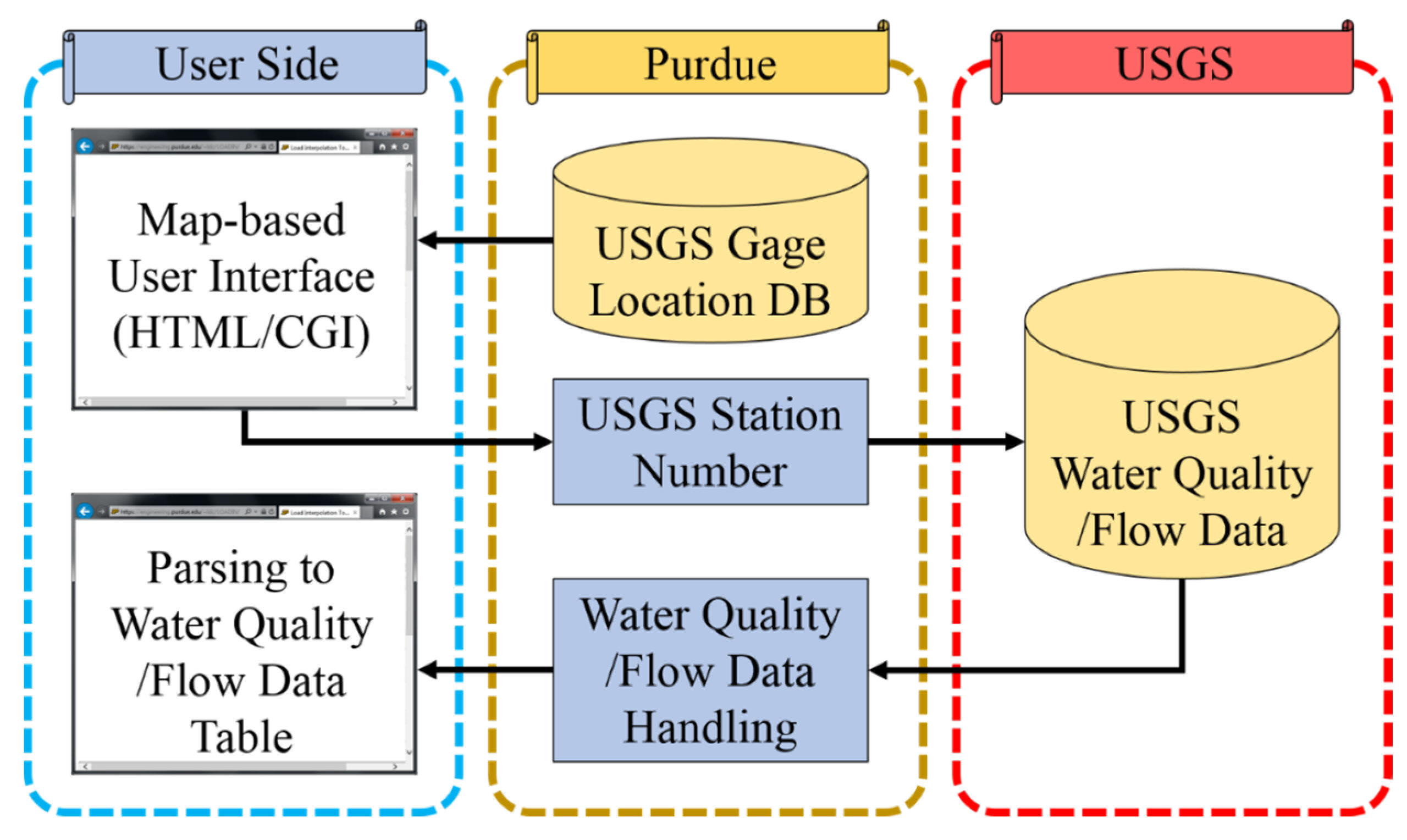
A web-based tool for pollutant load interpolation (LOADIN) [23] was developed in this study, providing features including automated, simple access of measured streamflow and water quality data via web access and no requirement for installation or updates of the tool on a desktop computer. LOADIN requires two inputs; one is streamflow data to calibrate the regression model coefficients and to estimate pollutant loads associated with streamflow. The other is water quality data. Therefore, the interface consists of two tables for the two inputs (Figure 1). The input data can be prepared by the user, or data can be prepared through web access to the U.S. Geological Survey (USGS). USGS allows web-access [24] to retrieve water quality; only USGS station number is required to request water quality data. LOADIN provides a map interface for the USGS gage stations for the entire U.S., using a database for the locations for streamflow water quality data built and stored in the web server (Figure 2). LOADIN displays the locations of USGS gage stations, requests water quality data from the USGS server as the user finds and selects the USGS station of interest on the map, and parses the data in the water quality data table.

Figure 1. LOADIN interface for streamflow and water quality data inputs.

Figure 1. LOADIN interface for streamflow and water quality data inputs.

Figure 2. Schematic depicting web-based tool access of water quality data from USGS server.

Figure 2. Schematic depicting web-based tool access of water quality data from USGS server.

2.2. Regression Model to Estimate Loads

LOADIN uses a regression model (Equation (1)) to estimate instantaneous load using streamflow, decimal time, and eight coefficients. The regression model is composed of three parts; the first part includes streamflow and model coefficients to represent pollutant loads for streamflow variation. The second part is comprised of streamflow, model coefficients, and decimal time with sine function. The third part is comprised of streamflow, model coefficients, and decimal time with cosine function. The second and third terms represent pollutant loads for time (or seasonal) variation. LOADIN, similar to LOADEST, uses a regression model to estimate pollutant loads. However, the regression model in LOADIN assumes that instantaneous load is comprised of the pollutant load from streamflow (i.e., Q_i in the Equation (1)) and the pollutant load variability for the given period as decimal time (i.e., T_i in the Equation (1)), whereas the regression models in LOADEST assume that instantaneous load is an exponential function of streamflow and pollutant load variability for the given period.

Park and Engel [22] and Park [25] applied the regression models in LOADIN and LOADEST to annual nitrogen, phosphorus, and sediment load estimation. Phosphorus and sediment data (mg/L) were related to streamflow data (m³/s), while nitrogen data (mg/L) displayed seasonal variance and generally poor relationships with streamflow data. The relationships between water quality and streamflow data led to different regression model behaviors. The regression model in LOADIN did not provide reasonable annual phosphorus and sediment load estimates, whereas the regression models in LOADEST did. In other words, the phosphorus and sediment loads followed the assumption of the regression models in LOADEST that pollutant loads are function of streamflow data. On the other hand, LOADEST provided poorer load estimates than LOADIN in annual nitrogen load estimation, since the nitrogen data displayed generally poor relationships with streamflow data. Thus it was concluded that streamflow and water quality datasets need to match the assumptions of regression models and that regression models need to be selected based on water quality parameters [20,21].

$${\text{Load}}_{\text{i}}={\text{C}}_0\cdot Q_i^{{\text{C}}_1}+{\text{ C}}_2\cdot \left[1+\text{sin}\left({\text{C}}_3\cdot T_i+{\text{C}}_4\right)\right]\cdot Q_i+{\text{ C}}_5\cdot [1+\text{cos}({\text{C}}_6\cdot T_i+{\text{C}}_7)]\cdot Q_i$$

(1)

where, Load_i is pollutant load at time step; i, C_0-7 are coefficients determined by an optimization algorithm; Q_i is streamflow at time step I; and T_i is decimal time streamflow measured.

LOADIN determines the eight coefficients that minimize differences between estimated and measured loads using a genetic algorithm. Developed by Holland [26], the genetic algorithm has solved sophisticated problems and has been applied for various areas, such as business, engineering, and science [27,28]. To determine the coefficients, three operators work through 500 generations, which are the selection operator to reproduce population with fitter individuals, the crossover operator to create offspring with combined strong individuals, and the mutation operator to alter partial characteristics of offspring at random. LOADIN calculates measured loads by multiplying water quality data by streamflow data associated with measured water quality data, and determines the regression model coefficients using a genetic algorithm that compares estimated loads from the regression model to measured loads on days measured loads are available.

3. Application of LOADIN

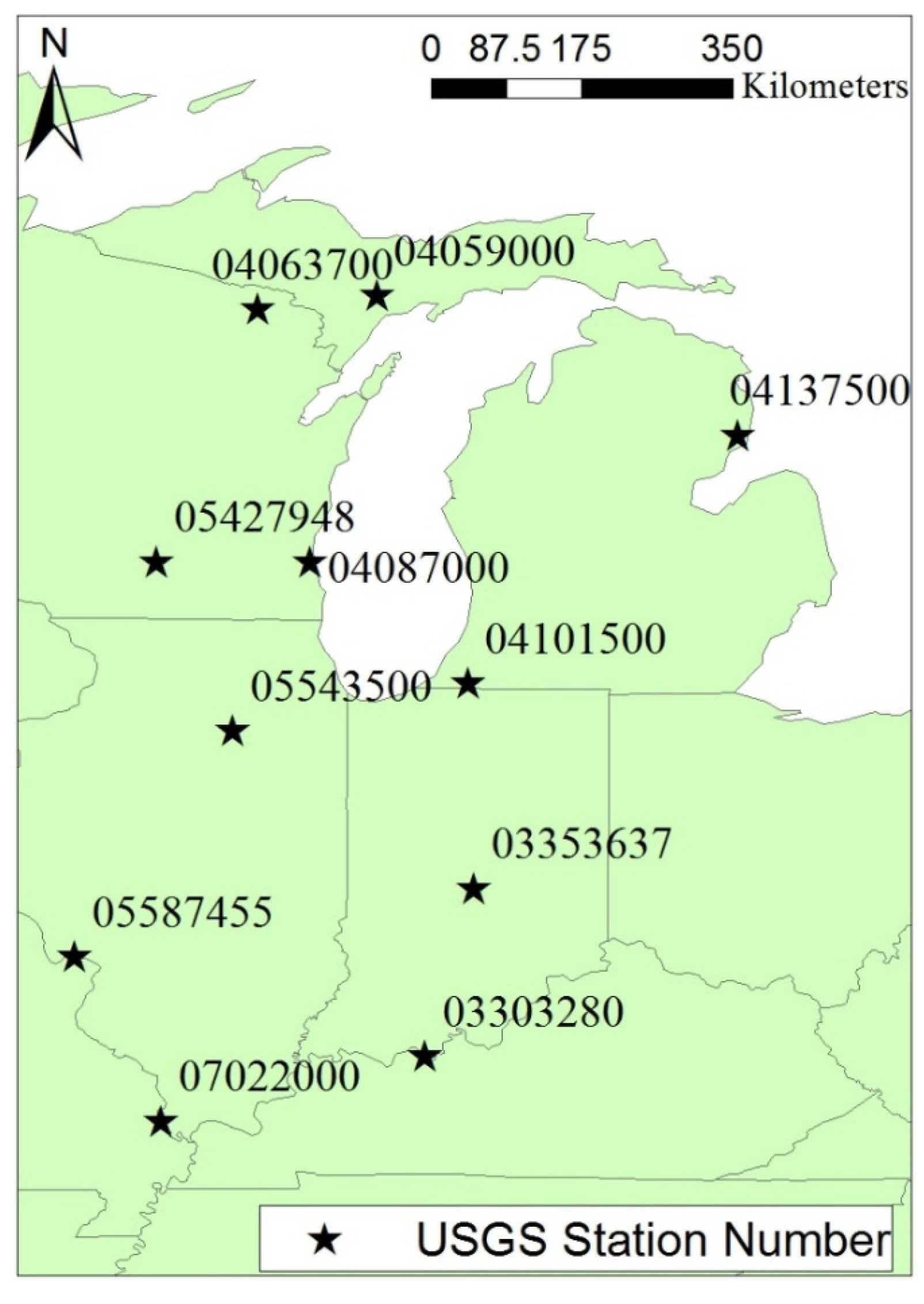
Since the regression model in LOADIN provided reasonable total nitrogen estimates, LOADN was applied to nitrogen data (USGS Water Quality Parameter Name: Nitrate plus nitrite, water, filtered, milligrams per liter as nitrogen, USGS Water Quality Parameter Code: 00631) from 11 USGS gage stations (Figure 3). The USGS gage stations are located in Illinois, Indiana, Michigan, Minnesota, and Wisconsin, and have drainage areas from 44 km² to 1,847,180 km² (Table 1). Since the drainage areas are different, the statistics of streamflow differed, with mean streamflow ranging from 0.6 m³/s (USGS Station Number 03353637) to 6772.4 m³/s (USGS Station Number 07022000).

Figure 3. Location of USGS stations for streamflow and nitrogen data.

Figure 3. Location of USGS stations for streamflow and nitrogen data.

Table 1. USGS locations and streamflow data statistics.

Station number	USGS station name	Drainage area (km2)	Data period	Streamflow (m3/s)
				Min.	Max.	Mean	Standard deviation
03353637	Little Buck Creek near Indianapolis, IN	44	17/05/1990–07/09/2004	0.01	39.36	0.60	1.54
05427948	Pheasant Branch at Middleton, WI	47	26/05/2009–17/06/2014	0.02	7.96	0.21	0.42
04063700	Popple river near Fence, WI	360	24/10/1979–10/06/2014	0.28	42.48	2.87	3.19
04087000	Milwaukee river at Milwaukee, WI	1803	18/09/1979–21/09/2009	0.23	254.00	15.06	17.77
04059000	Escanaba river at Cornell, MI	2253	26/09/1979–08/09/1994	4.25	294.50	22.65	22.95
04137500	Au Sable river near Au Sable, MI	4504	15/03/2011–09/09/2013	20.98	125.16	37.42	13.55
04101500	St. Joseph river at Niles, MI	9495	09/03/2011–16/06/2014	22.37	399.27	107.29	63.56
05543500	Illinois river at Marseilles, IL	21,391	25/09/1979–09/07/1998	58.62	2537.20	320.30	252.33
03303280	Ohio river at Cannelton dam at Cannelton, IN	251,229	17/01/1996–13/08/2013	72.21	20813.00	3997.84	3500.26
05587455	Mississippi river below Grafton, IL	443,665	16/10/1997–11/09/2013	379.45	12799.28	3665.40	2507.87
07022000	Mississippi River at Thebes, IL	1,847,180	26/07/1977–19/05/2014	1463.99	27694.03	6772.44	4200.45

Table 1. USGS locations and streamflow data statistics.

Station number	USGS station name	Drainage area (km2)	Data period	Streamflow (m3/s)
				Min.	Max.	Mean	Standard deviation
03353637	Little Buck Creek near Indianapolis, IN	44	17/05/1990–07/09/2004	0.01	39.36	0.60	1.54
05427948	Pheasant Branch at Middleton, WI	47	26/05/2009–17/06/2014	0.02	7.96	0.21	0.42
04063700	Popple river near Fence, WI	360	24/10/1979–10/06/2014	0.28	42.48	2.87	3.19
04087000	Milwaukee river at Milwaukee, WI	1803	18/09/1979–21/09/2009	0.23	254.00	15.06	17.77
04059000	Escanaba river at Cornell, MI	2253	26/09/1979–08/09/1994	4.25	294.50	22.65	22.95
04137500	Au Sable river near Au Sable, MI	4504	15/03/2011–09/09/2013	20.98	125.16	37.42	13.55
04101500	St. Joseph river at Niles, MI	9495	09/03/2011–16/06/2014	22.37	399.27	107.29	63.56
05543500	Illinois river at Marseilles, IL	21,391	25/09/1979–09/07/1998	58.62	2537.20	320.30	252.33
03303280	Ohio river at Cannelton dam at Cannelton, IN	251,229	17/01/1996–13/08/2013	72.21	20813.00	3997.84	3500.26
05587455	Mississippi river below Grafton, IL	443,665	16/10/1997–11/09/2013	379.45	12799.28	3665.40	2507.87
07022000	Mississippi River at Thebes, IL	1,847,180	26/07/1977–19/05/2014	1463.99	27694.03	6772.44	4200.45

Both streamflow and nitrogen data for the eleven USGS stations were retrieved by LOADIN, and the periods for nitrogen load estimates were defined based on the measured data. Streamflow were daily data, but nitrogen data intervals ranged from eight days (on average, USGS gage station 05427948) to fifty-nine days (on average, USGS gage station 04063700) (Table 2). Therefore, measured loads were calculated by multiplying nitrogen data by streamflow data associated with measured nitrogen data. The estimated nitrogen loads for the days which nitrogen data were measured were evaluated by Nash-Sutcliffe Efficiency (NSE) and coefficient of determination (R²) (Table 2; Figure 4). For example, 231 measured daily loads were computed by multiplying nitrogen concentration data by streamflow data, since USGS gage station 03353637 had 231 measured nitrogen data. The corresponding 231 estimated daily loads from 5228 estimated daily loads (i.e., same as the number of streamflow data) were extracted to compare estimated nitrogen loads to measured nitrogen loads on these days. The NSE of estimated nitrogen loads to measured nitrogen loads ranged from 0.45 (USGS gage station 05427948) to 0.91 (USGS gage station 04101500), and the R² ranged from 0.51 (USGS gage station 05427948) to 0.91 (USGS gage station 04101500) (Table 2; Figure 4b,g). More frequent nitrogen data (or large numbers of nitrogen data points) did not necessarily lead to higher NSE or R². For instance, the NSE and R² for USGS gage station 04101500 (63 nitrogen data points) were 0.91 and 0.91, respectively, however, the NSE and R² for USGS gage station 05427948 (218 nitrogen data points) were 0.45 and 0.51, respectively. In addition, drainage area was not related to the regression model behavior (Table 2; Figure 4b,g).

Table 2. Nash-Sutcliffe Efficiency (NSE) and coefficient of determination (R²) of estimated loads to measured load.

Station number	Number of data (Nitrogen/Streamflow)	Mean intervals of Nitrogen Data (days)	NSE	R2
03353637	231/5228	23	0.83	0.84
05427948	218/1850	8	0.45	0.51
04063700	215/12,597	59	0.52	0.58
04087000	253/10,963	43	0.84	0.84
04059000	98/5462	56	0.89	0.90
04137500	102/911	9	0.60	0.64
04101500	63/1193	19	0.91	0.91
05543500	154/6863	45	0.85	0.86
03303280	233/6421	28	0.88	0.88
05587455	210/5810	28	0.87	0.87
07022000	413/13,505	33	0.79	0.79

Table 2. Nash-Sutcliffe Efficiency (NSE) and coefficient of determination (R²) of estimated loads to measured load.

Station number	Number of data (Nitrogen/Streamflow)	Mean intervals of Nitrogen Data (days)	NSE	R2
03353637	231/5228	23	0.83	0.84
05427948	218/1850	8	0.45	0.51
04063700	215/12,597	59	0.52	0.58
04087000	253/10,963	43	0.84	0.84
04059000	98/5462	56	0.89	0.90
04137500	102/911	9	0.60	0.64
04101500	63/1193	19	0.91	0.91
05543500	154/6863	45	0.85	0.86
03303280	233/6421	28	0.88	0.88
05587455	210/5810	28	0.87	0.87
07022000	413/13,505	33	0.79	0.79

Figure 4. Scatter plots of measured and estimated nitrogen loads; (a) USGS station number 03353637; (b) USGS station number 05427948; (c) USGS station number 04063700; (d) USGS station number 04087000; (e) USGS station number 04059000; (f) USGS station number 04137500; (g) USGS station number 04101500; (h) USGS station number 05543500; (i) USGS station number 03303280; (j) USGS station number 05587455; (k) USGS station number 07022000.

Figure 4. Scatter plots of measured and estimated nitrogen loads; (a) USGS station number 03353637; (b) USGS station number 05427948; (c) USGS station number 04063700; (d) USGS station number 04087000; (e) USGS station number 04059000; (f) USGS station number 04137500; (g) USGS station number 04101500; (h) USGS station number 05543500; (i) USGS station number 03303280; (j) USGS station number 05587455; (k) USGS station number 07022000.

The regression model in LOADIN contains terms for time variation, and therefore the time distribution of nitrogen data collected was explored (Table 3). Sixty percent of nitrogen data in USGS gage station 05427948 was collected from March to June, and twenty percent of nitrogen data were collected in March. LOADIN provided poor load estimates for USGS gage station 05427948.

Similar to USGS gage station 05427948, forty-nine percent of nitrogen data were collected from March to June in USGS gage station 03303280, but the percentage for any month did not exceed thirteen percent. Therefore, the quantity of nitrogen data was not biased toward a certain month. Twenty-one percent of nitrogen data were collected in December for USGS gage station 04101500, but there were no consecutive months in which extensive nitrogen data were collected like USGS gage station 05427948. LOADIN provided reasonable load estimates for USGS gage stations 03303280 and 04101500.

If a water quality dataset is biased toward a certain period, LOADIN may provide poor load estimates. Since ten NSEs of the estimated loads to the measured loads, excluding for the nitrogen data from USGS station 05427948, were greater than 0.5, it was concluded that the LOADIN performed well in nitrogen load estimation [29], as long as the water quality dataset is not biased toward a certain period. For example, if nitrogen and streamflow datasets were collected only during summer, estimating nitrogen loads for winter using LOADIN should be avoided.

Table 3. Percentage of nitrogen data collected in each month.

Station Number	Percentage of nitrogen data collected (%)
	Jan.	Feb.	Mar.	Apr.	May	Jun.	Jul.	Aug.	Sep.	Oct.	Nov.	Dec.
03353637	6	4	6	6	15	16	14	14	7	3	4	5
05427948	6	9	20	14	14	12	4	3	4	3	5	6
04063700	6	7	8	10	8	11	6	12	9	7	10	8
04087000	5	6	9	8	11	13	11	9	9	7	7	6
04059000	12	3	10	9	8	10	7	7	11	6	10	5
04137500	8	2	15	19	8	7	4	3	4	11	6	15
04101500	8	8	8	19	6	6	6	5	3	3	6	21
05543500	6	8	8	9	11	6	8	13	7	6	10	7
03303280	11	9	12	12	12	13	4	8	3	2	6	7
05587455	6	8	10	10	9	11	8	8	7	8	8	7
07022000	5	6	10	12	14	11	11	8	7	7	4	5

Table 3. Percentage of nitrogen data collected in each month.

Station Number	Percentage of nitrogen data collected (%)
	Jan.	Feb.	Mar.	Apr.	May	Jun.	Jul.	Aug.	Sep.	Oct.	Nov.	Dec.
03353637	6	4	6	6	15	16	14	14	7	3	4	5
05427948	6	9	20	14	14	12	4	3	4	3	5	6
04063700	6	7	8	10	8	11	6	12	9	7	10	8
04087000	5	6	9	8	11	13	11	9	9	7	7	6
04059000	12	3	10	9	8	10	7	7	11	6	10	5
04137500	8	2	15	19	8	7	4	3	4	11	6	15
04101500	8	8	8	19	6	6	6	5	3	3	6	21
05543500	6	8	8	9	11	6	8	13	7	6	10	7
03303280	11	9	12	12	12	13	4	8	3	2	6	7
05587455	6	8	10	10	9	11	8	8	7	8	8	7
07022000	5	6	10	12	14	11	11	8	7	7	4	5

4. Conclusions

Although streamflow and water quality data associated with streamflow are required for pollutant load computations, collecting and analyzing water quality samples are costly and requires significant effort compared to streamflow data. Therefore, water quality data are often collected less frequently than streamflow data. Regression models are often used to estimate (or interpolate) pollutant loads from limited water quality and streamflow data.

A web-based tool, LOADIN, to interpolate pollutant loads was developed in the study. LOADIN has several benefits in pollutant load estimation. The first is that it is easy to operate and use the tool as no installation or update by the users is required since it is a web-based tool. The second is that LOADIN accesses nationwide streamflow and water quality data from the USGS via web access.

LOADIN uses a regression model assuming that instantaneous load is comprised of the pollutant load from streamflow and the pollutant load variability for the period. LOADIN was applied to eleven nitrogen datasets from USGS gage stations, and estimated nitrogen load was evaluated using NSE and R² based on measured nitrogen loads. Although LOADIN provided poor load estimation when the water quality dataset was biased toward a certain period, NSEs were greater than 0.5 in ten out of eleven USGS gage stations. Moreover, NSEs were greater than 0.8 for seven of the USGS gage stations. This indicates that LOADIN performance for nitrogen load estimations was satisfactory, unless the water quality dataset was biased toward a certain period.

References

- Coulter, C.B.; Kolka, R.K.; Thompson, J.A. Water quality in agricultural, urban, and mixed land use watershed. J. Am. Water Resour. Assoc. 2004, 40, 1593–1601. [Google Scholar]
- McMahon, G.; Harned, D.A. Effect of environmental setting on sediment, nitrogen, and phosphorus concentration in Albemarle-Pamlico Drainage Basin, North Carolina and Virginia, USA. Environ. Manag. 1998, 22, 887–903. [Google Scholar]
- Carey, R.O.; Migliaccio, K.W.; Brown, M.T. Nutrient discharges to Biscayne Bay, Florida: Trends, loads, and a pollutant index. Sci. Total Environ. 2011, 409, 530–539. [Google Scholar]
- Park, Y.S.; Engel, B.A.; Shin, Y.; Choi, J.; Kim, N.W.; Kim, S.J.; Kong, D.S.; Lim, K.J. Development of Web GIS-based VFSMOD System with three modules for effective vegetative filter strip design. Water 2013, 5, 1194–1210. [Google Scholar]
- Schelske, C.L.; Havens, K.E. The importance of considering biological processes when setting total maximum daily loads (TMDL) for phosphorus in shallow lakes and reservoirs. Environ. Pollut. 2001, 113, 1–9. [Google Scholar]
- Park, Y.S. Development and Enhancement of Web-Based Tools to Develop Total Maximum Daily Load. Ph.D. Thesis, Purdue University, West Lafayette, IN, USA, 18 May 2014; pp. 10–45. [Google Scholar]
- Engel, B.A.; Lim, K.J.; Hunter, J.; Chaubey, I.; Quansah, J.E.; Theller, L.; Park, Y.S. Web-Based LDC Tool User’s Guide; Purdue University: West Lafayette, IN, USA, 2014. [Google Scholar]
- Robertson, D.M. Influence of different temporal sampling strategies on estimating total phosphorus and suspended sediment concentration and transport in small streams. J. Am. Water Resour. Assoc. 2003, 39, 1281–1308. [Google Scholar]
- Horowitz, A.J. An evaluation of sediment rating curves for estimating suspended sediment concentrations for subsequent flux calculations. Hydrol. Proc. 2003, 17, 3387–3409. [Google Scholar]
- Robertson, D.M.; Roerish, E.E. Influence of various water quality sampling strategies on load estimates for small streams. Water Resour. Res. 1999, 35, 3747–3759. [Google Scholar]
- Harmel, R.D.; King, K.W.; Haggard, B.E.; Wren, D.G.; Sheridan, J.M. Practical guidance for discharge and water quality data collection on small watershed. Trans. Am. Soc. Agric. Eng. 2006, 49, 937–948. [Google Scholar]
- Gilroy, E.J.; Hirsch, R.M.; Cohn, T.A. Mean square error of regression-based constituent transport estimates. Water Resour. Res. 1990, 26, 2069–2077. [Google Scholar]
- Cohn, T.A.; DeLong, L.L.; Gilroy, E.J.; Hirsh, R.M.; Wells, D.K. Estimating constituent loads. Water Resour. Res. 1989, 25, 937–942. [Google Scholar]
- Cohn, T.A.; Caulder, D.L.; Gilroy, E.J.; Zynjuk, L.D.; Summers, R.M. The validity of a simple statistical model for estimating fluvial constituent loads: An empirical study involving nutrient loads entering Chesapeake Bay. Water Resour. Res. 1992, 28, 2353–2363. [Google Scholar]
- Runkel, R.L.; Crawford, C.G.; Cohn, T.A. Load Estimator (LOADEST): A Fortran Program for Estimating Constituent Loads in Streams and Rivers; U.S. Geological Survey Techniques and Methods: Reston, VA, USA, 2004. [Google Scholar]
- Maret, T.R.; MacCoy, D.E.; Carlisle, D.M. Long-term water quality and biological responses to multiple best management practices in Rock Creek, Idaho. J. Am. Water Resour. Assoc. 2008, 44, 1248–1269. [Google Scholar]
- Duan, S.; Kaushal, S.S.; Groffman, P.M.; Band, L.E.; Belt, K.T. Phosphorus export across an urban to rural gradient in the Chesapeake Bay watershed. J. Geophys. Res. 2012, 117. [Google Scholar] [CrossRef]
- Brigham, M.E.; Wentz, D.A.; Aiken, G.R.; Krabbenhoft, D.P. Mercury cycling in stream ecosystems. 1. Water column chemistry and transport. Environ. Sci. Technol. 2009, 43, 2720–2725. [Google Scholar]
- Dornblaser, M.M.; Striegl, R.G. Suspended sediment and carbonate transport in the Yukon River basin, Alska: Flouxes and potential future responses to climate change. Water Resour. Res. 2009, 45. [Google Scholar] [CrossRef]
- Oh, J.; Sankarasubramanian, A. Interannual hydroclimatic variability and its influence on winter nutrients variability over the southeast United States. Hydrol. Earth Syst. Sci. Discuss. 2011, 8, 10935–10971. [Google Scholar]
- Park, Y.S.; Engel, B.A.; Harbor, J. A web-based model to estimate the impact of best management practices. Water 2014, 6, 455–471. [Google Scholar]
- Park, Y.S.; Engel, B.A. Use of pollutant load regression models with various sampling frequencies for annual load estimation. Water 2014, 6, 1685–1697. [Google Scholar]
- Web-based Load Interpolation Tool. Available online: https://engineering.purdue.edu/~ldc/LOADIN (accessed on 21 July 2014).
- USGS Water-Quality Data for the Nation. Available online: http://waterdata.usgs.gov/nwis/qw (accessed on 23 March 2013).
- Park, Y.S. Development and enhancement of web-based tools to develop Total Maximum Daily Load. Ph.D. Thesis, Purdue University: West Lafayette, IN, USA, 2014; 10–70. [Google Scholar]
- Holland, J.H. Adaptation in Natural and Artificial Systems; University of Michigan Press: Ann Arbor, MI, USA, 1975. [Google Scholar]
- Park, Y.S.; Kim, J.; Kim, N.W.; Kim, S.J.; Jeon, J.H.; Engel, B.A.; Jang, W.S.; Lim, K.J. Development of new R, C, and SDR modules for the SATEEC GIS system. Comput. Geosci. 2010, 36, 726–734. [Google Scholar]
- Lim, K.J.; Park, Y.S.; Kim, J.; Shin, Y.C.; Kim, N.W.; Kim, S.J.; Jeon, J.H.; Engel, B.A. Development of genetic algorithm-based optimization module in WHAT system for hydrolograph analysis and model application. Comput. Geosci. 2010, 36, 936–944. [Google Scholar]
- Moriasi, D.N.; Arnold, J.G.; Van Liew, M.W.; Bingner, R.L.; Harmel, R.D.; Veith, T.L. Model evaluation guidelines for systematic quantification of accuracy in watershed simulations. Trans. Am. Soc. Agric. Eng. 2007, 50, 885–900. [Google Scholar]
© 2014 by the authors; licensee MDPI, Basel, Switzerland. This article is an open access article distributed under the terms and conditions of the Creative Commons Attribution license (http://creativecommons.org/licenses/by/3.0/).
Share and Cite
MDPI and ACS Style
Park, Y.S.; Engel, B.A. A Web-Based Tool to Interpolate Nitrogen Loading Using a Genetic Algorithm. Water 2014, 6, 2770-2781. https://doi.org/10.3390/w6092770
AMA Style
Park YS, Engel BA. A Web-Based Tool to Interpolate Nitrogen Loading Using a Genetic Algorithm. Water. 2014; 6(9):2770-2781. https://doi.org/10.3390/w6092770
Chicago/Turabian StylePark, Youn Shik, and Bernie A. Engel. 2014. "A Web-Based Tool to Interpolate Nitrogen Loading Using a Genetic Algorithm" Water 6, no. 9: 2770-2781. https://doi.org/10.3390/w6092770