1. Introduction
In the western United States, water scarcity has resulted in a heavy dependency on groundwater to meet public and domestic drinking water demands [
1]. Growing populations and the changing climate will continue to increase the need for groundwater in these regions [
2]. With the further development of groundwater resources comes the potential to deplete surface waters, in particular streams and rivers. This process is known as stream depletion and it occurs because of the hydraulic connection between ground and surface water. Pumping groundwater from an aquifer forms a cone of hydraulic head depression around the well. Near a losing stream, this cone of depression steepens the hydraulic head gradient away from the stream. This leads to an increase in the flow of water from the losing stream to the aquifer, and therefore to stream depletion. Near a gaining stream, the cone of depression causes the well to intercept baseflow that would otherwise contribute to the stream, thereby causing stream depletion. In some scenarios, the cone of depression may be sufficiently steep to convert a gaining stream to a losing stream.
The legality of impacting surface water flow via groundwater extraction is dependent upon the established water rights within each state. For example, water rights defined by the State of Colorado distinguish between groundwater that contributes to surface water flow, called tributary groundwater, and groundwater that does not contribute to surface water flow, called non-tributary groundwater. If a source is determined to be tributary groundwater, it is regulated under the same legislative rights as surface water. Conversely, non-tributary groundwater is not subject to the same water rights system as surface water [
3].
Distinctions between tributary and non-tributary groundwater are made using either analytical or numerical estimations of stream depletion. Analytical estimations of stream depletion were first proposed by Theis [
4] and have since continued to be developed (e.g., [
5,
6,
7,
8,
9,
10]). However, Spalding and Khaleel [
11] demonstrated that, despite their convenience, analytical approaches often fail to account for conditions that exist in natural steam-aquifer systems. Since that time, numerical groundwater models have proven to more accurately estimate stream depletion as they can better account for the complex nature of true systems [
12,
13,
14,
15,
16].
Numerical models of stream depletion solve the groundwater flow equation, which, for an unconfined aquifer, is given by
where
h is aquifer head,
x = (
x, y) is the spatial coordinate,
t is time,
Sy is specific yield,
K is the hydraulic conductivity tensor,
ζ is the elevation of the aquifer bottom,
Qp is the pumping rate,
xw is the pumping well location,
Kr and
br are the hydraulic conductivity and thickness, respectively, of the streambed sediment,
w is the width of the stream,
hs is the head in the stream,
xs(
y) is the
x-coordinate of the center of the stream as a function of
y, and
W includes all other sources and sinks of water. For simplicity of notation, we assume that the river runs in the
y direction, although this assumption is not necessary. In stream depletion applications, this equation is commonly solved with MODFLOW [
17].
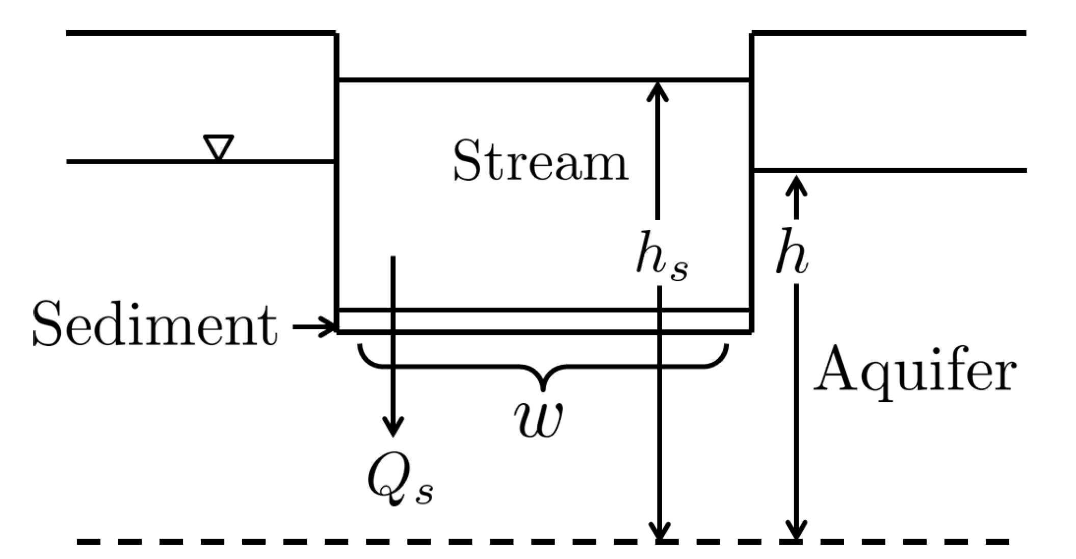
Figure 1 represents the streambed as it is interpreted by the MODFLOW stream (STR) package.
In this figure,
Qs represents flow across the streambed, which is calculated using Darcy’s law through
where
L is the length of stream reach, and
C is the streambed conductance, which combines the hydraulic properties and geometry of the streambed. The magnitude of
C indicates the degree to which the stream and the aquifer are connected. Thus, streams with large
C are strongly connected to the underlying aquifer.
Figure 1.
Cross-sectional view of the stream as it is interpreted by the STR package of MODFLOW. The hydraulic head of the stream (hs) and aquifer (h) are shown with respect to a datum that is represented as a dashed line. The flow across the streambed (Qs) as well as the width of the streambed (w) are also shown.
If we let
Qr be the flow rate in the stream reach of interest, then the change in this flow rate due to pumping, denoted as ∆
Qr, is defined as stream depletion. The flow rate
Qr depends on the flow rate of water into the stream reach from an upstream reach, flow
Qs across the streambed as shown in Equation (2), precipitation, evaporation, and direct inflows from surface runoff along the reach. Of these flow components, only
Qs is affected by pumping; thus, the stream depletion ∆
Qr is identical to the change in
Qs. This relationship is described by
Equation (3) shows that the stream depletion depends on streambed conductance
C and on the change in the hydraulic head difference between the stream and the aquifer. For a given change in the head difference, a higher
C leads to a greater degree of stream depletion and a lower
C leads to a lesser degree of stream depletion [
13,
14]. The correlation between
C and the stream depletion makes it an important model parameter in numerical stream depletion simulations (e.g., [
9,
10,
11,
12,
18,
19]).
Along the length of a stream, the streambed naturally exhibits spatial variability of
C [
20,
21,
22,
23,
24,
25,
26,
27,
28], which, combined with aquifer heterogeneity, has been shown to affect the small scale and intermediate scale water fluxes between the stream and the aquifer. In a field investigation of fluxes along a stream reach that is 60 m long, Conant [
29] found the fluxes can vary significantly in both magnitude and direction. Fleckenstein
et al. [
30] used numerical simulations to investigate the effects of aquifer heterogeneity on water fluxes in a 10 km by 40 km domain around a river. They found that aquifer heterogeneity on the scale of 100 m significantly impacted the spatial distribution of water fluxes between the river and the aquifer. Kalbus
et al. [
31] investigated the effects of both aquifer and streambed heterogeneity on the small scale water fluxes (on the scale of 1 m), and they found that the aquifer heterogeneity plays a more significant role than the streambed heterogeneity.
While these and related studies [
32] have shown that aquifer and streambed heterogeneity at small to intermediate scales can lead to spatial variability of water fluxes at those same scales, the implications of these heterogeneities on stream depletion estimates have not been considered. Stream depletion analyses consider the change in the total flow rate in a stream, which is manifested as the integrated effect of the change in water fluxes over the entire stretch of a stream that is impacted by pumping. Thus, the small scale spatial variations in the water fluxes between a stream and an aquifer are of interest only in how they impact the overall change in flow rate. For this reason, the effects of small to intermediate scale aquifer and streambed heterogeneities are expected to be less influential on stream depletion than the larger scale heterogeneities.
Typically, large scale groundwater flow models that are used to simulate stream depletion deem the streambed as homogeneous, with property values that are assumed or calibrated (e.g., [
33]). Specifically, it is often the case that the value of streambed hydraulic conductivity used in the simulation is not based on any physical measurements, but rather on an assumed or calibrated value. If this value is not representative of the physical system, the estimates of stream depletion may be incorrect. Furthermore, if a heterogeneous streambed is modeled as a homogeneous streambed, the estimates of stream depletion produced by the model may be misleading.
Several studies have evaluated the effects of using an incorrect assumption of streambed heterogeneity in numerical simulations to estimate water fluxes between a river and an aquifer. A key factor in the simulation of fluxes is the degree of connection between the river and the aquifer. If the water table is above the elevation of the river bottom, complete hydraulic connection exists between the river and the aquifer. If the water table is sufficiently far below the river bottom such that the river and aquifer are completely disconnected, the water flux from the river to the aquifer reaches a maximum value and becomes independent of the aquifer water level. Between these two states the hydraulic connection is transitional [
34]. Irvine
et al. [
35] compared the degree of connection and the water flux between an aquifer and a 20 m by 20 m section of a hypothetical losing river with a heterogeneous streambed, and between an aquifer and the same river with a homogeneous streambed and equivalent water fluxes. They found that the accuracy of the predicted fluxes with the homogeneous streambed model depended on the degree of connection between the river and aquifer at the calibrated state and on whether the water table was rising or falling. Errors in water flux were negligible for rising water tables if the aquifer and river were connected at the calibrated state and for falling water tables if the aquifer and river were completely disconnected at the calibrated state. For other combinations of degree of connection at the calibration state and direction of movement of the water table, the estimated water fluxes could be both overpredicted or underpredicted, by as much as 35%, depending on the streambed heterogeneity. Kurtz
et al. [
36] performed a similar investigation on a larger scale, using a model of the Limmat valley aquifer in Zurich, Switzerland. They compared water fluxes from the fully heterogeneous riverbed to water fluxes from an equivalent homogeneous riverbed and from rivers with two, three, or five leakage zones and found that the degree of accuracy of predicted water fluxes decreased as the simulated level of heterogeneity decreased.
The goal of this study is to investigate the effects of large scale streambed heterogeneity on the calculation of stream depletion. In this work, we conceptually expand on the fundamental analytical solutions of stream depletion through groundwater pumping provided in [
5,
6,
7,
8,
9,
10] by applying MODFLOW to investigate the impact of assuming or calibrating for a homogeneous
C on regional scale stream depletion estimates. Although MODFLOW makes several simplifying assumptions that may produce errors in estimates of water flux between a river and an aquifer [
37], we use MODFLOW in this work because it is commonly used in simulations to estimate stream depletion. We define a homogeneous, rectangular domain with an area of 1280 km
2, with no-flow boundaries on three sides, a fixed head boundary at the southern end, and steady, uniform recharge across the domain. Aquifer heterogeneity is not considered, so that the effects of streambed heterogeneity on stream depletion can be isolated. All locations in the domain are considered potential well locations. A sinusoidal stream runs from north to south along the center of the domain. We start by investigating the sensitivity of stream depletion to the streambed conductance
C for a homogeneous streambed. We then determine the range of
C to which stream depletion is sensitive, and we investigate how this sensitive range of
C is impacted by pumping well placement and aquifer hydraulic conductivity. Consequently, we apply spatial
C heterogeneity, by varying
C over two orders of magnitude, to assess the impact of streambed heterogeneity on regional scale estimates of stream depletion. The practical implications of the spatial variability of
C are assessed through a comparison of the heterogeneous scenarios with a homogeneous base case.
2. Conceptual Model
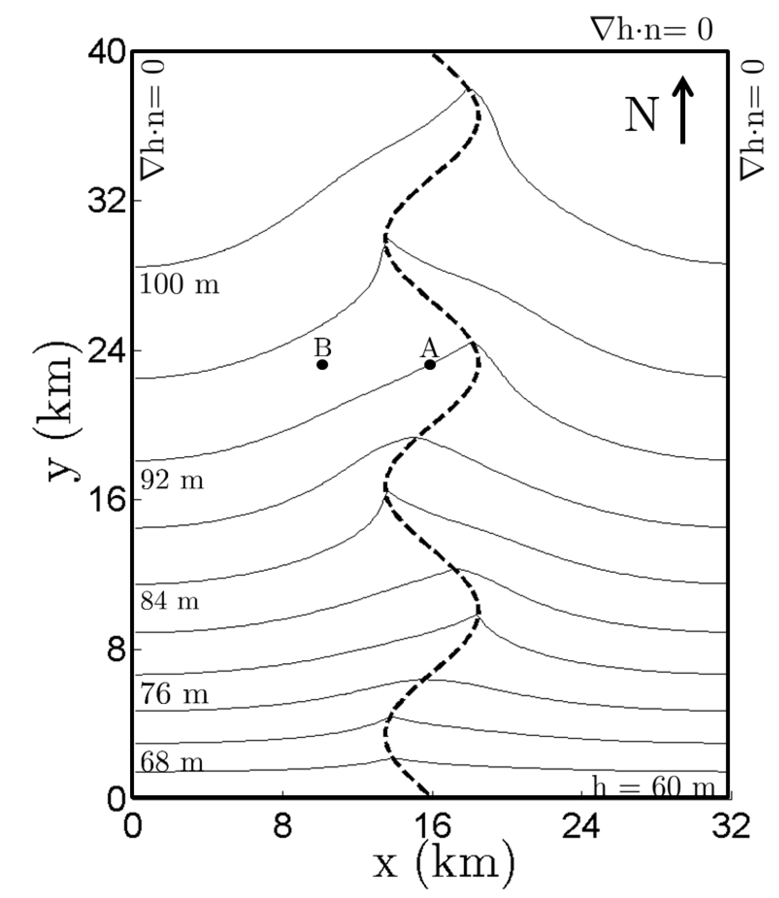
The base model is an isotropic, homogeneous, unconfined aquifer through which water flows from north to south. A plan view of the model area, the steady state hydraulic head, pumping well locations, and the model boundary conditions are shown in
Figure 2. No-flow boundary conditions were assumed on the north, east, and west boundaries and a constant head boundary of
h = 60 m on the southern boundary. Water enters the model through evenly distributed recharge of 4
× 10
−5 m d
−1 (1.5 cm per year). Flow is horizontal in the unconfined aquifer and the Dupuit assumptions are maintained. A meandering stream flows through the model from north to south and is simulated with the stream package in MODFLOW. This stream gains water from the aquifer along its length and maintains a flow depth of approximately 1.5 m. For all of our simulations, streambed conductance
C is varied through the streambed hydraulic conductivity,
Kr . A summary of key model parameters is provided in
Table 1.
This work investigates the depletion of the stream at the southern boundary of the model. Groundwater enters the aquifer through natural recharge across the basin and exits the model domain through three boundaries: a single pumping well, the stream, and the downstream constant head boundary that represents the neighboring groundwater basin and may also be a source of water to the well. Pumped water initially comes from aquifer storage, but over time as the cone of depression expands, the pumped water also comes from the stream depletion and from a reduction in outflow at the southern boundary. The proportion of the pumped water that comes from the stream depletion or from a reduction in outflow depends on the hydraulic properties of the aquifer and the stream, the geometry of the streambed, and the location of the pumping well. We deliberately chose the domain geometry and recharge rate of our hypothetical model to represent conditions that potentially lead to significant stream depletion.
Figure 2.
Plan view of steady state head distribution in the modeled aquifer with K = 5 m d−1 and a homogeneous Kr = 0.003 m d−1. Pumping is not considered in this scenario; however, pumping well locations are represented at points A (x, y) = (15.875 km, 23.175 km) and B (x, y) = (9.875 km, 23.175 km). The boundary conditions are shown on the model boundaries and the stream is represented by a dashed line.
Table 1.
Aquifer and model parameters.
Table 1.
Aquifer and model parameters.
| Description | Value |
|---|
| Head at south boundary, at
y = 0 m | 60 m |
| Elevation of aquifer bottom | 0 m |
| Recharge rate | 4
× 10−5 m d−1 |
| Stream bottom elevation at north boundary | 98.5 m |
| Stream bottom at south boundary | 58.5 m |
| Streambed slope | 0.00077 |
| Manning’s coefficient of roughness for the streambed | 0.04 d m
−1/3 |
| Spatial discretization | 250 m
× 250 m |
| Pumping rate (
Qp) | 100 m3 d
−1 |
| Specific yield | 0.2 |
| Stream width (
w) | 10 m |
| Streambed thickness (br) | 0.3 m |
To calculate the stream depletion due to pumping from a single well at any location in the aquifer, a simulation is run without any pumping wells, and the simulated value of Qs is recorded at the time of interest. Then, the simulation is repeated with pumping at a well at the location of interest, and the new simulated value of Qs is recorded. The difference between these two values of Qs is the stream depletion. In this study, we present normalized stream depletion results measured as a fraction of the pumping rate (∆Qr/Qp).
3. Sensitivity of Stream Depletion Estimates to Streambed Conductance
Multiple studies have shown that stream depletion is sensitive to streambed conductance (e.g., [
9,
13,
14,
19,
30]), while others have demonstrated an insensitivity of stream depletion to
C (e.g., [
33]). In this section, we demonstrate the relationship between stream depletion and streambed conductance to illustrate that there exist a range of streambed conductance values to which stream depletion is sensitive. Although the streambed is assumed to be homogeneous in this section, these simulation results demonstrate the expected limiting cases of stream depletion for a heterogeneous streambed that is discussed in the next section.
Figure 3 shows the estimates of normalized stream depletion, ∆
Qr/Qp, as a function of time for the four scenarios described in
Table 2 for 29 different values of
Kr (or equivalently, 29 different values of
C), ranging from 10
−4 m d
−1 to 10
3 m d
−1 with an increment of 0.25 log units. This range of
Kr was identified by [
38] as the range of observed
Kr in 41 field and modeling studies that assessed or used the parameter. These results were obtained by solving Equation (1) using MODFLOW, with the parameters shown in
Table 1. In all cases, the stream depletion increases over time at a decreasing rate, and a larger
Kr leads to a higher degree of stream depletion than a smaller
Kr. For example, in
Figure 3a, the normalized stream depletion after 100 years of pumping is ∆
Qr/Qp = 0.0363 for
Kr = 10
−4 m d
−1 (circle) and is ∆
Qr/Qp = 0.9424 for
Kr = 10
−0.25 m d
−1 (diamond). For a higher
Kr, the hydraulic connection between the aquifer and the stream is increased; thus, the water from the stream more easily flows across the streambed to replenish the water removed from the aquifer due to pumping. This behavior is consistent with the results of Hunt [
9] and Christensen [
19], who considered a straight, infinitely long stream in an infinite aquifer.
Figure 3 also shows that for a given
Kr, normalized stream depletion decreases as the distance between the pumping well and the stream increases (compare subplots a and b), since the drawdown in the vicinity of the stream is lower for a more distant pumping well. Furthermore,
Figure 3 shows that for a given pumping well location and
Kr, the stream depletion decreases as the aquifer hydraulic conductivity increases (compare subplots a, c, and d). This behavior agrees with the finding of Christensen [
19], who showed that the sensitivity of drawdown to aquifer transmissivity varies with time and depends on the ratio of streambed conductance to aquifer transmissivity.
Figure 3 demonstrates that, for each scenario, there exist a range of
Kr values for which the stream depletion significantly changes for a small change in
Kr (between dashed lines), and other ranges of
Kr for which the stream depletion barely changes for a large change in
Kr (above the upper dashed line and below the lower dashed line). We arbitrarily define this sensitive
Kr range as the range for which
Figure 3.
Normalized stream depletion vs. time for (a) Well A with K = 5 m d−1; (b) Well B with K = 5 m d−1; (c) Well A with K = 10 m d−1; and (d) Well A with K = 2.5 m d−1. Each set of results shows the stream depletion estimates for 29 streambeds with a spectrum of Kr that varies from 10−4 m d−1 (corresponding to the lowest stream depletion) to 103 m d−1 (corresponding to the highest stream depletion). For Kr > 10−1 m d−1, the curves are visually indistinguishable. The dashed curves represent the upper and lower boundaries of the range of Kr to which the stream depletion estimates are sensitive.
Table 2.
Model parameters and sensitive Kr range for each scenario.
Table 2.
Model parameters and sensitive Kr range for each scenario.
| Scenario | Well Location | K (m d−1) | Sensitive
Kr Range (m d−1) |
|---|
| a | A: (15.875 km, 23.175 km) | 5 | 10
−3.75 to 10−1.75 |
| b | B: ( 9.875 km, 23.175 km) | 5 | 10
−3.5 to 10−1.5 |
| c | A: (15.875 km, 23.175 km) | 10 | 10
−3.75 to 10−1.5 |
| d | A: (15.875 km, 23.175 km) | 2.5 | 10
−3.75 to 10−1.75 |
Table 2 shows the sensitive
Kr ranges for each of the four scenarios, which span approximately two orders of magnitude. The range of observed
Kr from [
38] spans seven orders of magnitude; therefore, for most values in the realistic range of
Kr, the stream depletion is not sensitive to
Kr. These ranges depend on both the distance between the stream and the pumping well and the aquifer hydraulic conductivity, consistent with the findings of Christensen [
19].
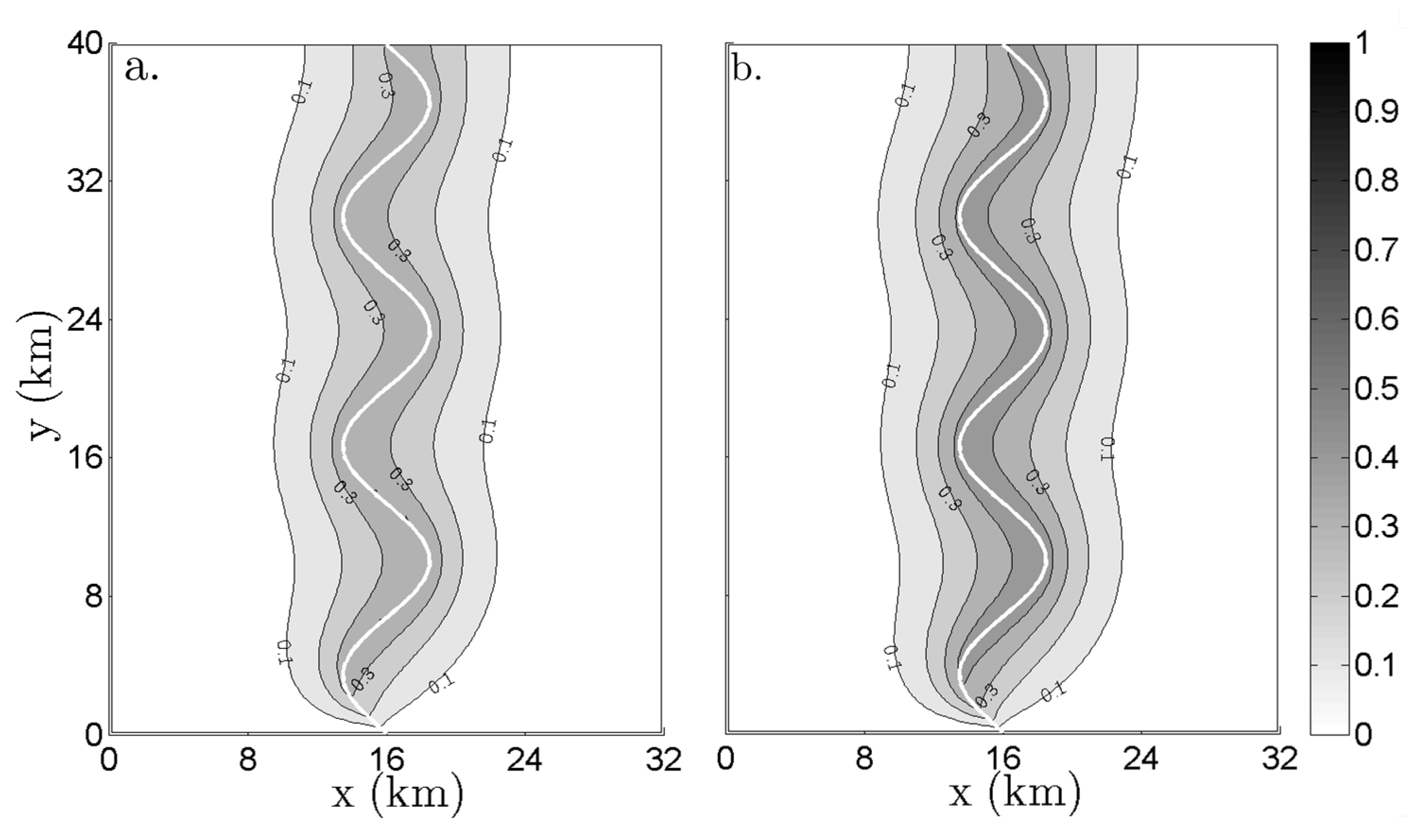
Legal or environmental restrictions often limit the degree to which a pumping well may deplete a stream. If a location of a new well is to be chosen, simulations can be used to estimate the stream depletion that would result from pumping at any location in the aquifer, as shown in
Figure 4. The gray shade corresponds to the normalized stream depletion, ∆
Qr/Qp, that would result from pumping from a well at that location for 20 years in an aquifer with a
K value of 5 m d
−1. For these simulations, Equation (1) was solved using the adjoint approach [
39], using a homogeneous streambed with
Kr = 3
× 10
−3 m d
−1 (
Figure 4a) and
Kr = 4
× 10
−3 m d
−1 (
Figure 4b). Both of these
Kr values are within the sensitive
Kr range for Scenario (a),
Figure 3a.
Figure 4.
Normalized stream depletion (∆Qr/Qp) in an aquifer with K = 5 m d−1 and a homogeneous streambed with (a) Kr = 3 × 10⁻³ m d−1 and (b) Kr = 4 × 10⁻³ m d−1 after 20 years of pumping.
Figure 4.
Normalized stream depletion (∆Qr/Qp) in an aquifer with K = 5 m d−1 and a homogeneous streambed with (a) Kr = 3 × 10⁻³ m d−1 and (b) Kr = 4 × 10⁻³ m d−1 after 20 years of pumping.
4. Effects of Streambed Heterogeneity on Stream Depletion Estimates
Due to natural streambed heterogeneity, spatial variations of
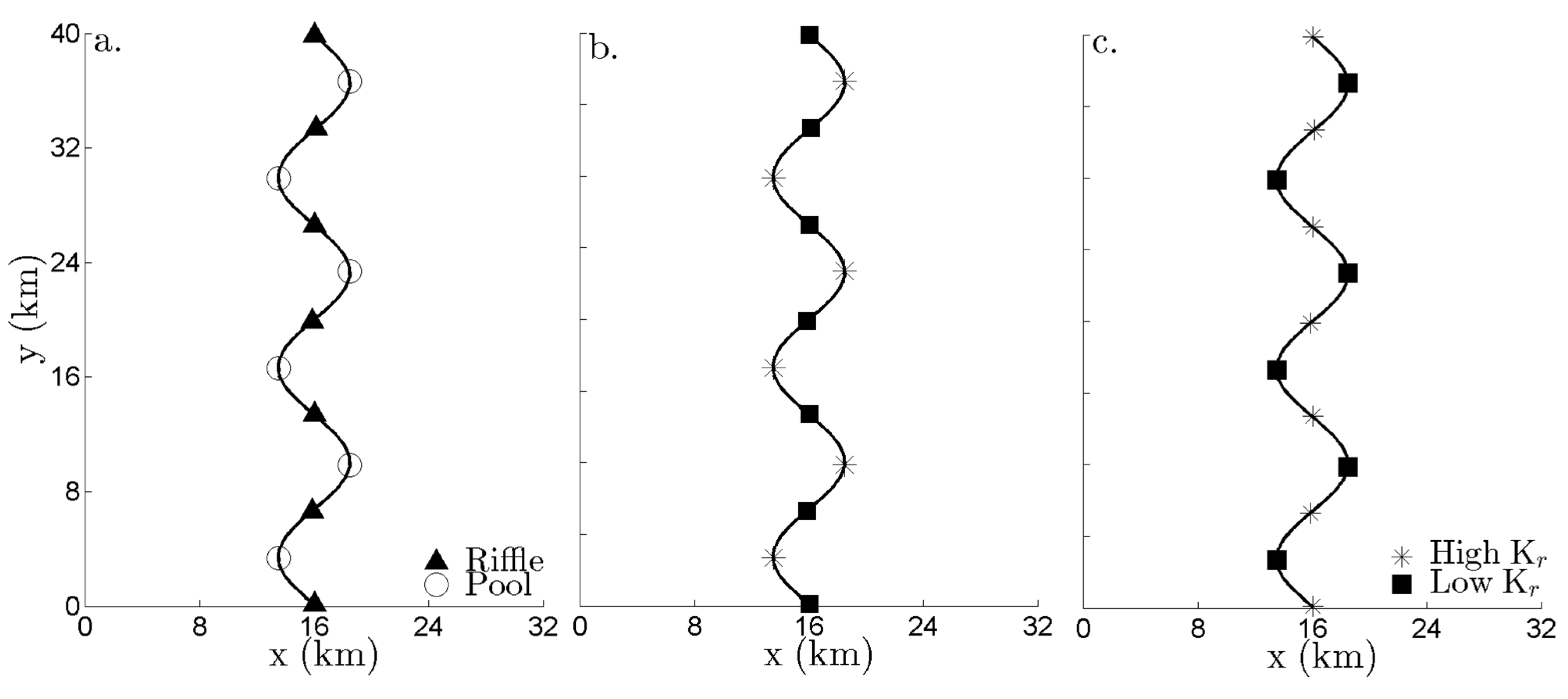
Kr often occur along a single streambed. In this section, the impact of this heterogeneity on regional scale stream depletion estimates is assessed assuming that the streambed is comprised of a sequence of pools and riffles. The bends of the stream are designated as pools and the straight sections are designated as riffles (
Figure 5a). Pools and riffles exhibit different sediment transport behavior based on the flow regime. The model used in this study is that under the high flow regime, sediments scour from pools and are deposited in riffles, whereas under the low flow regime the opposite behavior is observed [
40]. The sections of the streambed that are scouring and filling are represented with regions of high
Kr and low
Kr , respectively. Thus, high and low flow conditions create different patterns of streambed
Kr.
Figure 5.
Plan view of the modeled aquifer, showing (a) the assumed pool and riffle sequence; (b) the streambed Kr pattern under high flow regime conditions; and (c) the streambed Kr pattern under low flow regime conditions.
Figure 5.
Plan view of the modeled aquifer, showing (a) the assumed pool and riffle sequence; (b) the streambed Kr pattern under high flow regime conditions; and (c) the streambed Kr pattern under low flow regime conditions.
To model the streambed under the high flow regime, we varied
Kr linearly over two orders of magnitude along the streambed between a high
Kr at the point of maximum curvature and a low
Kr at the point of minimum curvature (
Figure 5b). The
Kr pattern was reversed for the low flow regime, resulting in a high
Kr at the minimum point of curvature that is two orders of magnitude larger than the low
Kr at the maximum point of curvature (
Figure 5c).
For each combination of flow regime and mean
Kr, we calculated the stream depletion due to pumping at any location in an aquifer with
K = 5 m d
−1.
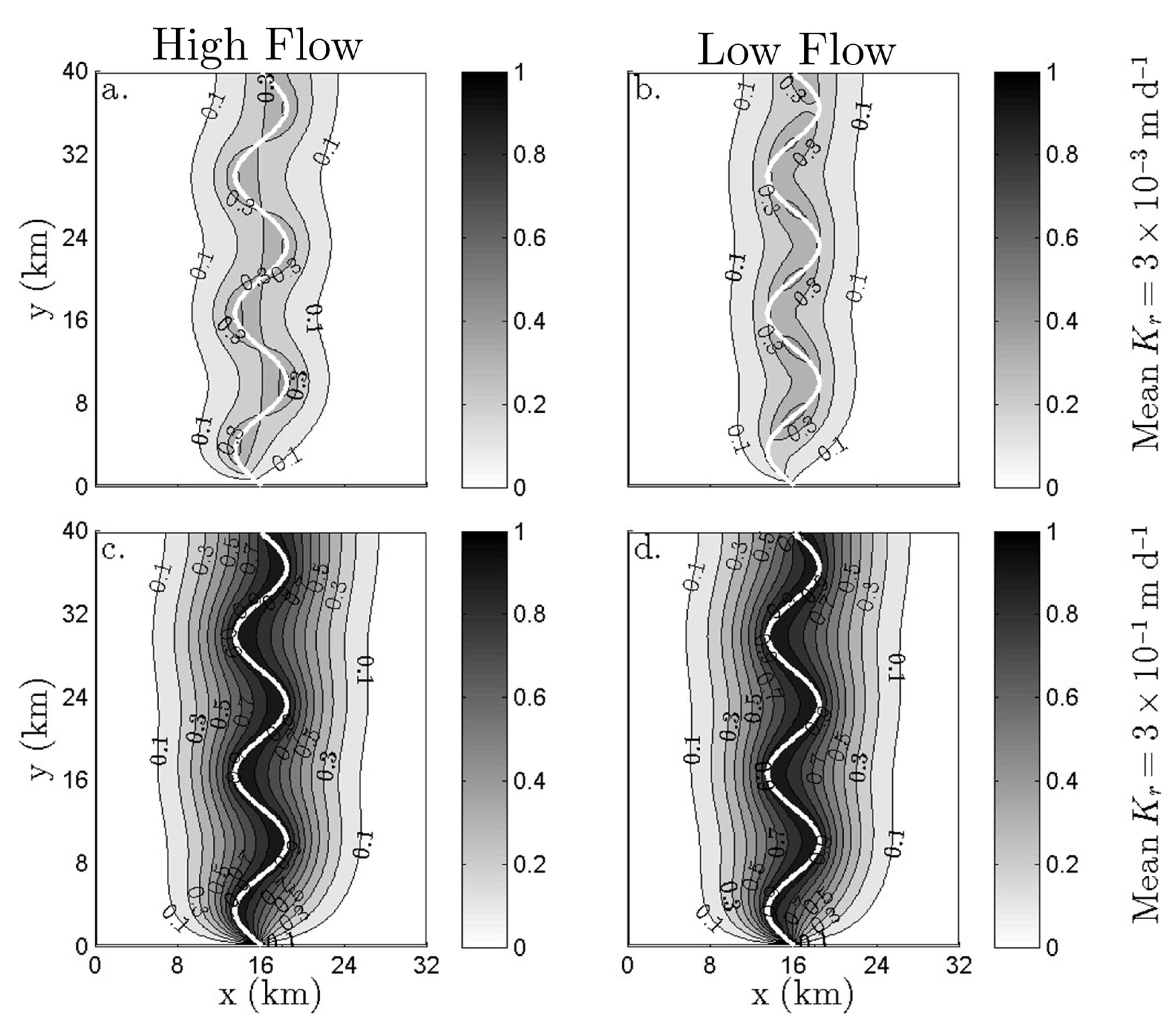
Figure 6a,b shows the stream depletion in a stream with a mean
Kr of 3
× 10
−3 m d
−1, which is within the sensitive
Kr range for spatial
Kr variability for high flow and low flow regimes, respectively. As shown in Equation (2), the stream depletion is directly proportional to
Kr. Thus, pumping within regions of the aquifer near streambed sections with high
Kr leads to a greater degree of stream depletion, while pumping in regions near low
Kr reaches leads to a lesser degree of stream depletion. This results in a greater degree of stream depletion for pumping from wells near the stream bends for the high flow regime (
Figure 6a), and a greater degree of stream depletion or pumping from wells near the straight sections for the low flow regime (
Figure 6b).
Figure 6c,d shows stream depletion for the same scenarios as
Figure 6a,b, except that the mean
Kr is changed to
Kr = 0.3 m d
−1, which is above the sensitive range. In this case, the spatial patterns of the stream depletion for the high flow (
Figure 6c) and low flow (
Figure 6d) regimes are visually indistinguishable. In fact, for this case, the spatial pattern of stream depletion is similar to the pattern for a homogeneous streambed (
Figure 4). The stream depletion decreases with the distance from the stream independently of the position along the stream channel. These results show that for stream depletion simulations, the streambed may be modeled as homogeneous if
Kr is outside of the sensitive range, but the heterogeneity should be modeled if
Kr is within the sensitive
Kr range.
Figure 6.
Normalized stream depletion (∆Qr/Qp) at each potential well location in an aquifer with K = 5 m d−1 for four heterogeneous scenarios after 20 years of pumping.
Figure 6.
Normalized stream depletion (∆Qr/Qp) at each potential well location in an aquifer with K = 5 m d−1 for four heterogeneous scenarios after 20 years of pumping.
High flow regime with mean Kr = 3 × 10⁻³ m d−1 (within sensitive range); (b) Low flow regime with mean Kr = 3 × 10⁻³ m d−1 (within sensitive range); (c) High flow regime with mean Kr = 3 × 10⁻¹ m d−1 (above sensitive range); (d) Low flow regime with mean Kr = 3 × 10⁻¹ m d−1 (above sensitive range).
5. Discussion
Regional scale numerical simulations of stream depletion are typically performed for regulatory purposes, often to identify areas of an aquifer where groundwater pumping can take place without having an undesirable amount of stream depletion in a nearby stream. For illustrative purposes, we define two limits of normalized stream depletion: ∆Qr/Qp = 0.1 and ∆Qr/Qp = 0.3. For each scenario, regions of the aquifer where pumping depletes the stream by less than the limit are considered feasible locations for a pumping well, and regions where pumping depletes the stream beyond the limit are considered infeasible locations.
As stated earlier, although natural streambeds are heterogeneous, they are often deemed homogeneous in stream depletion simulations. In
Figure 7, we compare the infeasible region that would be identified from assuming a homogeneous streambed with the infeasible regions obtained using a heterogeneous streambed from the high flow regime (
Figure 7a), a heterogeneous streambed from the low flow regime (
Figure 7b), and a homogeneous streambed with a higher
Kr (
Figure 7c).
Figure 7.
Normalized stream depletion due to pumping at every well location in the model domain for a homogeneous streambed after 20 years of pumping. The thick solid line represents the boundary of the region of infeasible locations for pumping wells if the streambed is homogeneous with Kr = 0.003 m d−1. The thick dashed line represents the boundary of the region of infeasible pumping well locations for (a) heterogeneous Kr(high flow regime) with mean Kr = 0.003 m d−1; (b) heterogeneous Kr (low flow regime) with mean Kr = 0.003 m d−1; and (c) homogeneous Kr with mean Kr = 0.004 m d−1.
Considering the limit of ∆
Qr/Qp = 0.3, all three scenarios in
Figure 7 show feasible pumping regions that differ from the base case. For the high flow regime, the high
Kr at the stream bends creates a region of infeasible well locations that is slightly wider near the bends and narrower near the straight sections than the region of infeasible well locations for the base case. This trend is reversed for the low flow regime, where the heterogeneous
Kr creates a region of infeasible well locations that is narrower along the bends and slightly wider along the straight section. The homogeneous scenario with larger
Kr has an infeasible region that is larger than the base case along the entire length of the stream channel.
Considering the limit of ∆
Qr/Qp = 0.1, the infeasible pumping region extends farther away from the stream in all considered scenarios.
Figure 7 shows minimal differences between the infeasible pumping region of the base case and the infeasible pumping regions of the high flow and low flow scenarios. The boundary of the infeasible pumping region obtained using a higher, homogeneous
Kr is again larger than for the base case. These results show that the size and shape of the infeasible pumping region will be affected by the spatial variation in
Kr for some choices of the limit and unaffected for some others, and thus the assumption of a homogeneous streambed may be acceptable in certain cases. These results also illustrate that if the true value of
Kr falls within the sensitive range, and if the homogeneous value of
Kr used in the model is incorrect, the infeasible pumping region identified by the model will be misleading. Stream depletion is an averaging process, whereby the changes in stream-aquifer fluxes are averaged over the extent of the cone of depression of the well. Although streambed heterogeneities may occur on scales smaller than what we use here, for scales of heterogeneity smaller than that of the cone of depression, the effects of heterogeneity average out, and stream depletion is more similar to what would be observed from a homogeneous streambed. For any well location, stream depletion occurs when the cone of depression reaches the stream. Thus, if the scale of heterogeneity is
λ, the wells within a distance of approximately
λ from the stream would be influenced by streambed heterogeneity (for example, within ∆
Qr/Qp = 0.3 in
Figure 7a), whereas the wells outside of a distance of approximately
λ from the stream would not be influenced by streambed heterogeneity (for example, outside of ∆
Qr/Qp = 0.1 in
Figure 7a).
In this study, we investigated the effects of streambed heterogeneity on stream depletion in a gaining stream in a basin with relatively low recharge. Although the results of the study cannot necessarily be generalized to all stream-aquifer systems, the results can be extended beyond the conceptual model investigated here. For example, a low recharge rate was used in our model; however, stream depletion is not affected by increases in recharge, unless it leads to a significant increase in the saturated thickness of the unconfined aquifer. Thus, similar behavior is expected for small changes in recharge. On the other hand, in a domain with a losing river, lowering the recharge may cause the water table to drop to a level where it becomes hydraulically disconnected from the stream, which would significantly alter the stream depletion estimates. In this work, we used a pumping rate of Qp = 100 m3 d−1. Normalized stream depletion (∆Qr/Qp) is independent of pumping rate as long as the cone of depression around the pumping well does not lower the water table below the bottom of the stream channel and is not significantly influenced by the boundary conditions. With larger aquifer hydraulic conductivity, the cone of depression would be larger, thus the influence of the model boundaries would extend farther into the domain.
Our work explores the effects of using an incorrect representation of streambed hydraulic properties in a model that simulates stream depletion. Since a model is a simplification of reality, it may misrepresent other components of the physical system as well, which can also lead to errors in stream depletion estimates. For example, regional groundwater flow models often assume two-dimensional flow, although groundwater flow in the vicinity of the stream is known to be three-dimensional [
41]. Also, intermediate scale aquifer heterogeneity can significantly influence the spatial distribution of river seepage [
30], at least on an intermediate scale. Thus, estimates of stream depletion using a heterogeneous, two-dimensional flow model may be incorrect.
6. Conclusions
In this study, we considered the effects of streambed conductance (C) on stream depletion estimates. We varied C through streambed hydraulic conductivity (Kr). For a given model, a range of Kr values exist to which stream depletion estimates are sensitive. If the true Kr is within the sensitive Kr range, then a small variation between the modeled Kr and the true Kr may lead to stream depletion estimates that are significantly different than the real system stream depletion. If the true Kr is above or below the sensitive range, slight variations in Kr will have no impact on the stream depletion estimates. Considering the uncertainty introduced from parameter assumption or calibration, the assessment of model sensitivity to the proposed Kr should be an essential step in the development of a stream depletion model.
We also demonstrated that the values of
Kr to which the model is sensitive depend on the aquifer hydraulic conductivity (
K) as well as the distance between the pumping well and the stream. Stream depletion reduces when aquifer
K is increased or the pumping well is located farther away from the stream. These two parameters alter the size of the sensitive
Kr range as well as the magnitude of
Kr within the sensitive
Kr range. These findings are consistent with results of other studies [
9,
19].
Natural streambeds are heterogeneous and typically have Kr that varies over several orders of magnitude. The significance of accounting for this Kr heterogeneity in numerical stream depletion simulations was also investigated in this work. We considered a stream comprised of a simplified sequence of pools and riffles to develop patterns of Kr heterogeneity along the streambed for the high and low flow regimes. Our results show that the spatial pattern of heterogeneous Kr have the potential to significantly impact the degree of stream depletion estimated for pumping well locations near the stream if the mean Kr is within the sensitive Kr range.
We assessed the practical impact of streambed Kr on stream depletion by comparing the region of infeasible pumping well locations under a variety of streambed Kr scenarios with the infeasible region of a homogeneous base case. We demonstrated the significance of using an accurate Kr when the true Kr is within the sensitive Kr range of the model. We showed that near the stream, the shape of the region of infeasible pumping well locations is affected by the magnitude and spatial variability of Kr. This effect is subdued as distance from the stream increases. Therefore, modeling the Kr heterogeneity is less critical if the pumping well locations near the stream are not considered. For a homogeneous stream channel with Kr inside the sensitive Kr range, it is critical that the value of Kr deployed in the model truly represents the genuine Kr. In general, a high Kr leads to a better connection between the stream and aquifer, which results in more stream depletion and extends the boundary of the region of infeasible pumping well locations farther away from the stream. Thus, an incorrectly simulated value of Kr can significantly alter the size of the infeasible pumping region.


