
Estimation of Rainfall Associated with Typhoons over the Ocean Using TRMM/TMI and Numerical Models

Abstract
:1. Introduction
2. Theory


3. Methodology
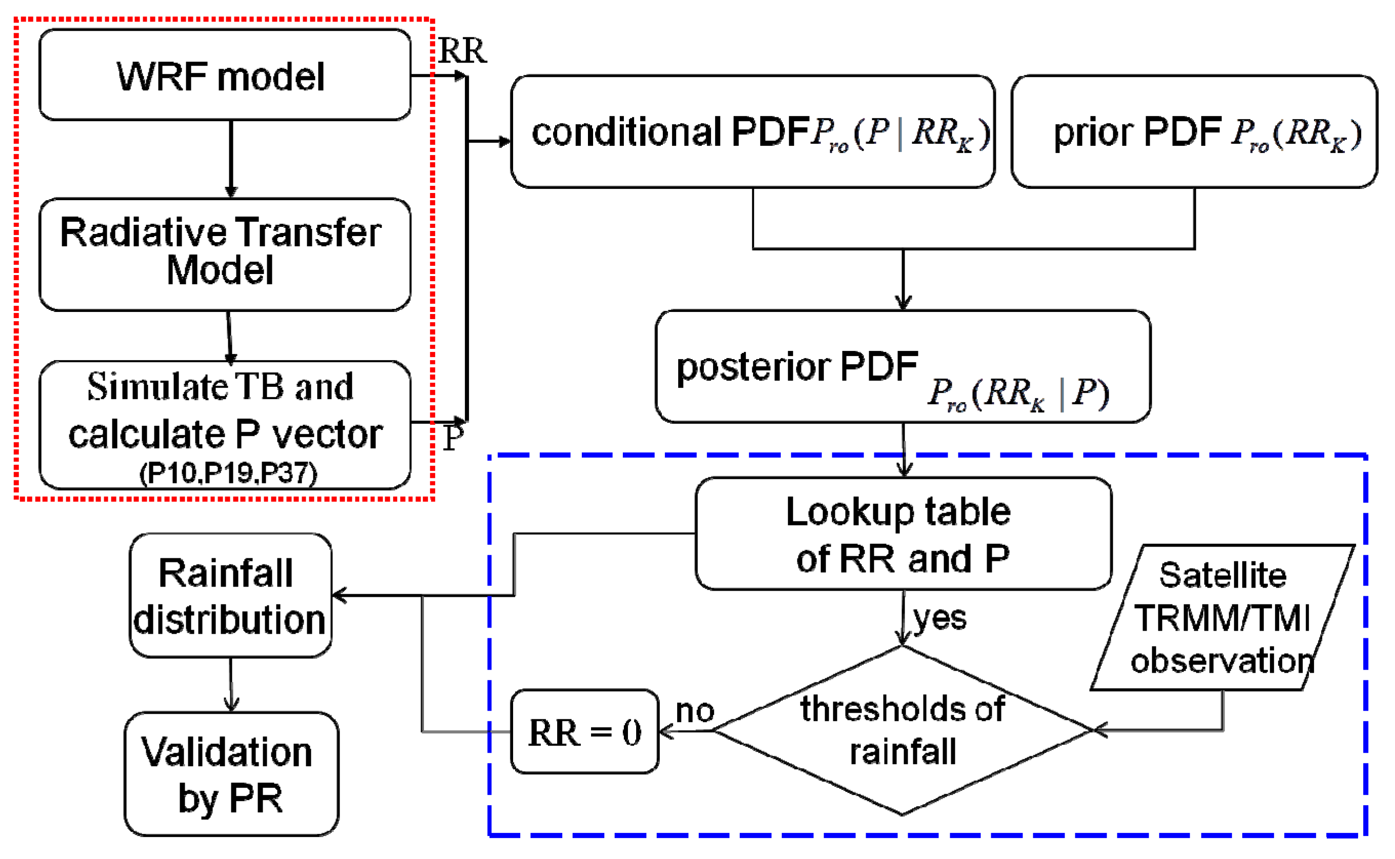
3.1. Physical Algorithm
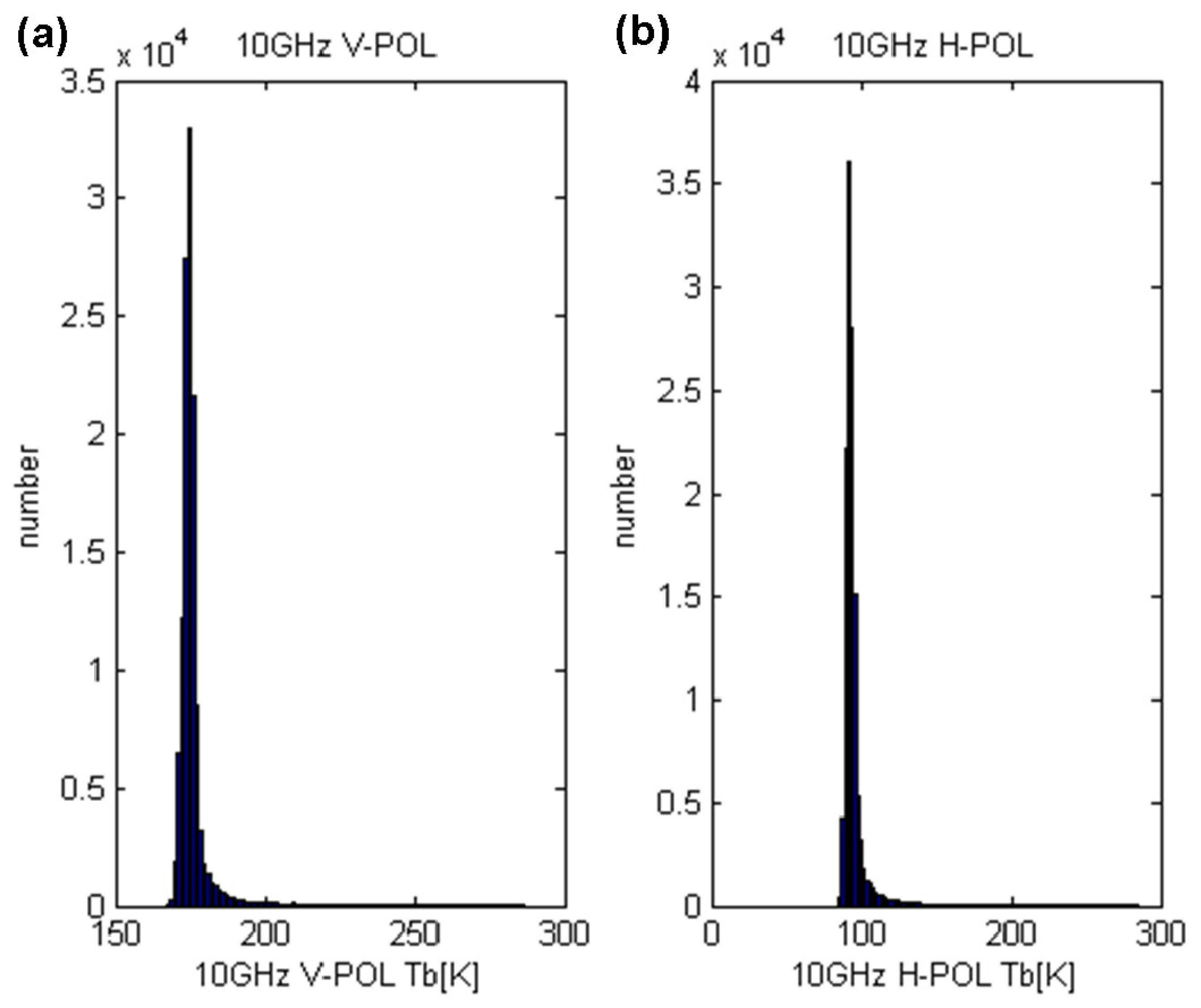
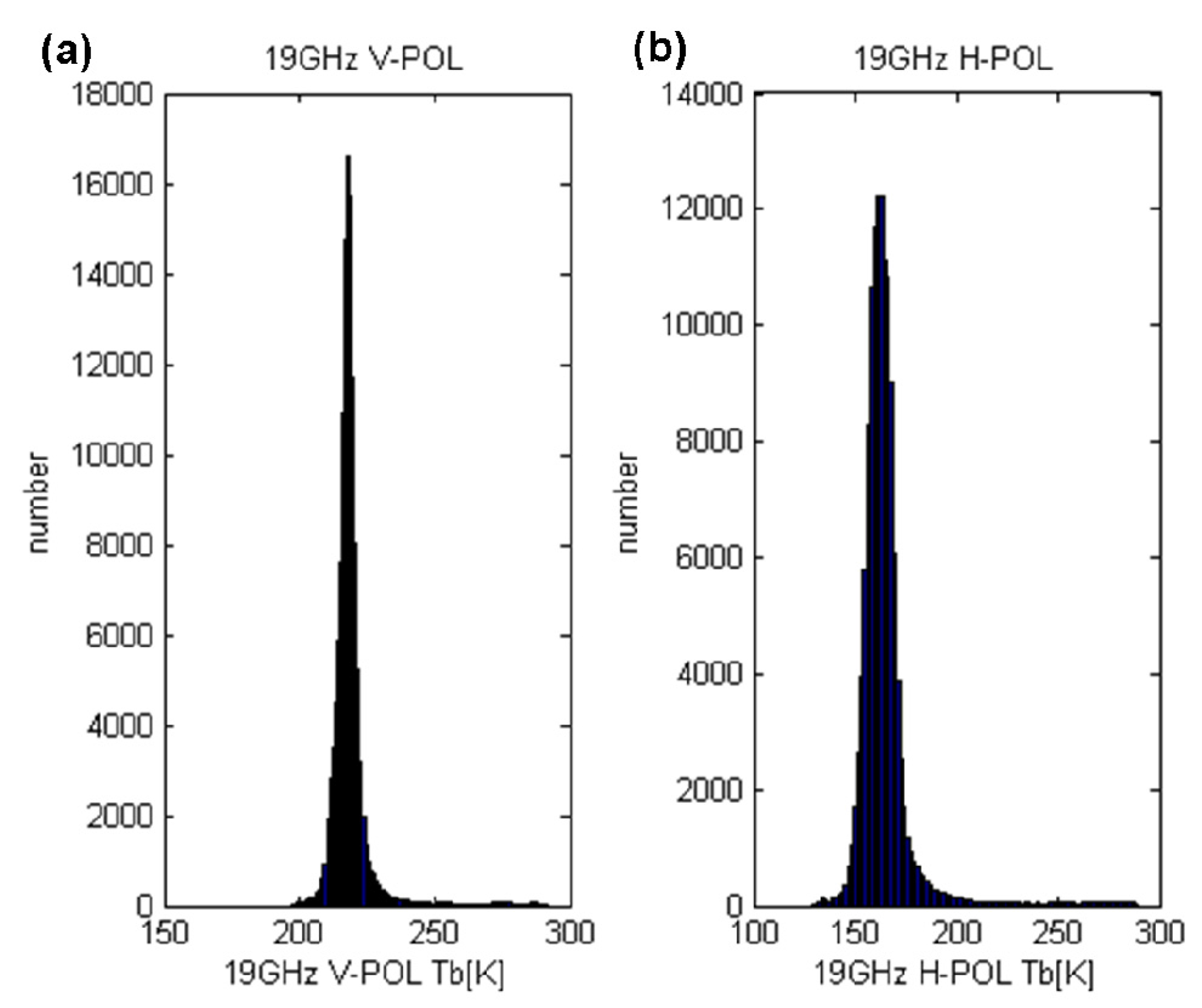
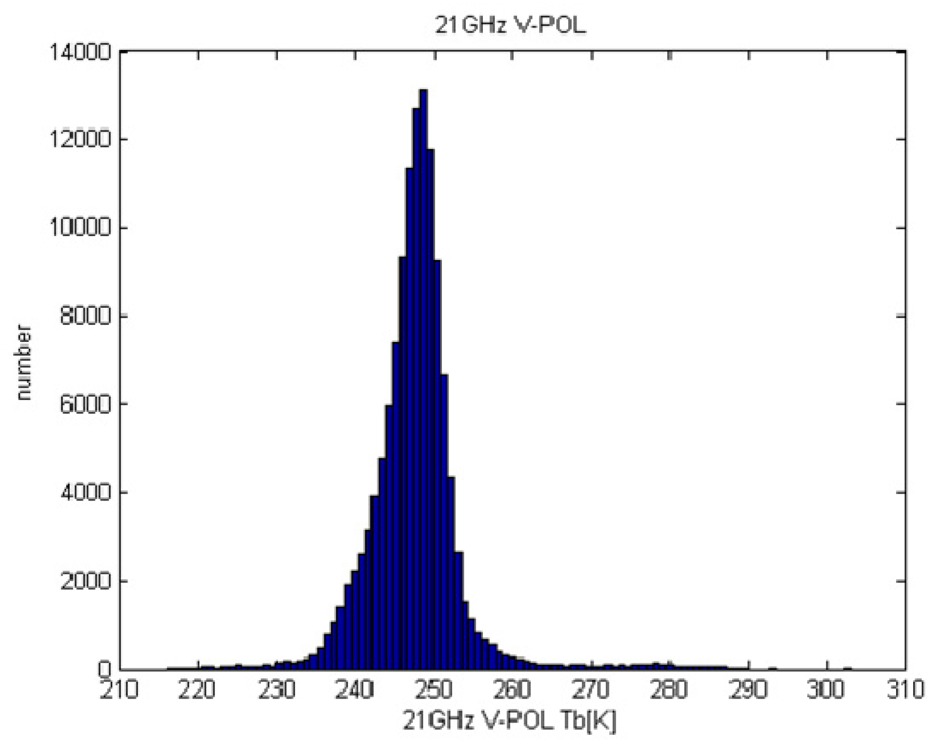
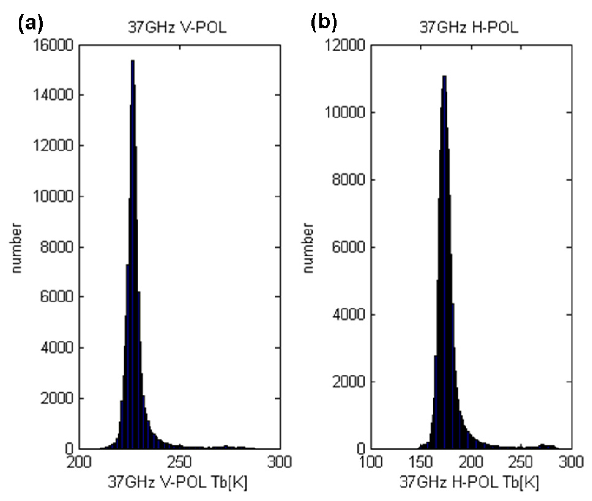
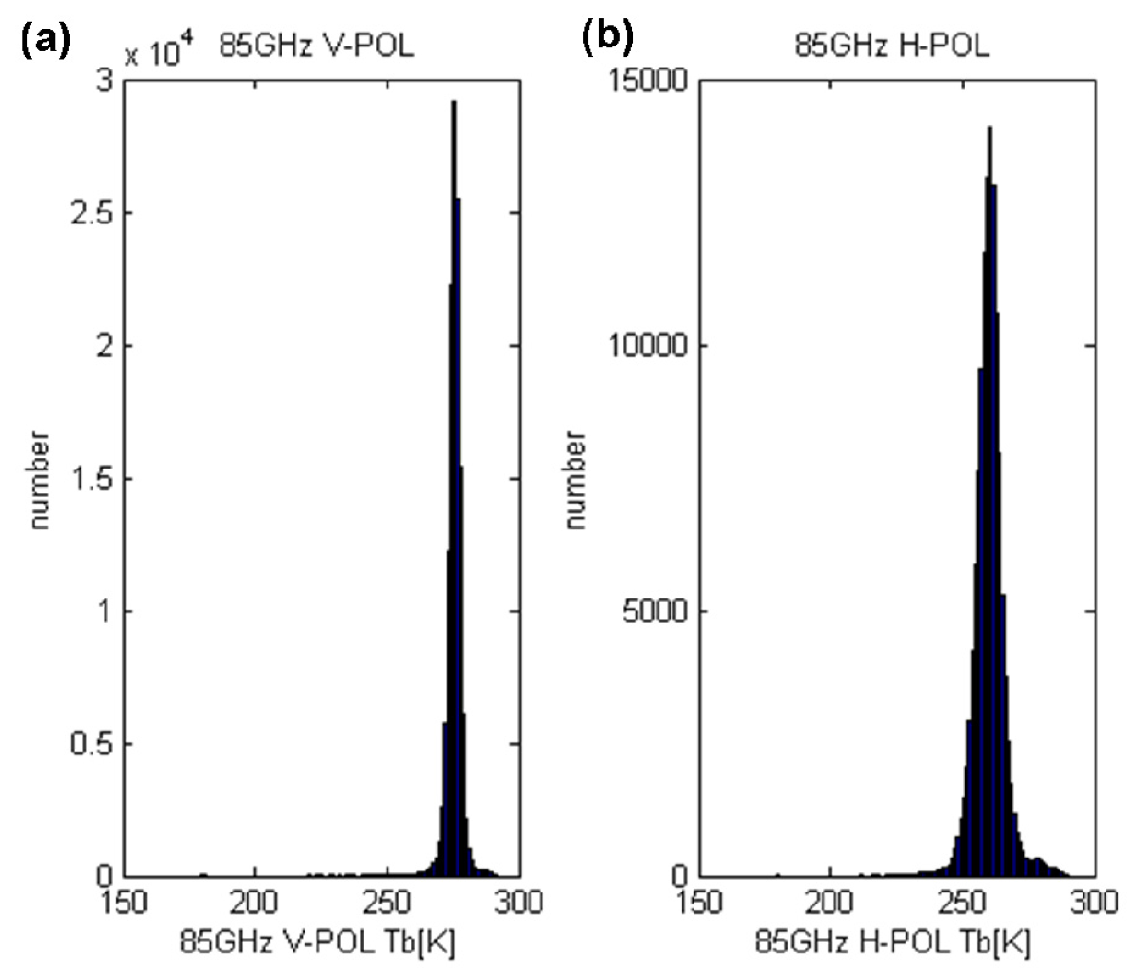
3.2. Establishing a Threshold for Rain


| Frequencies | Threshold (Mean) | Standard Deviation |
|---|---|---|
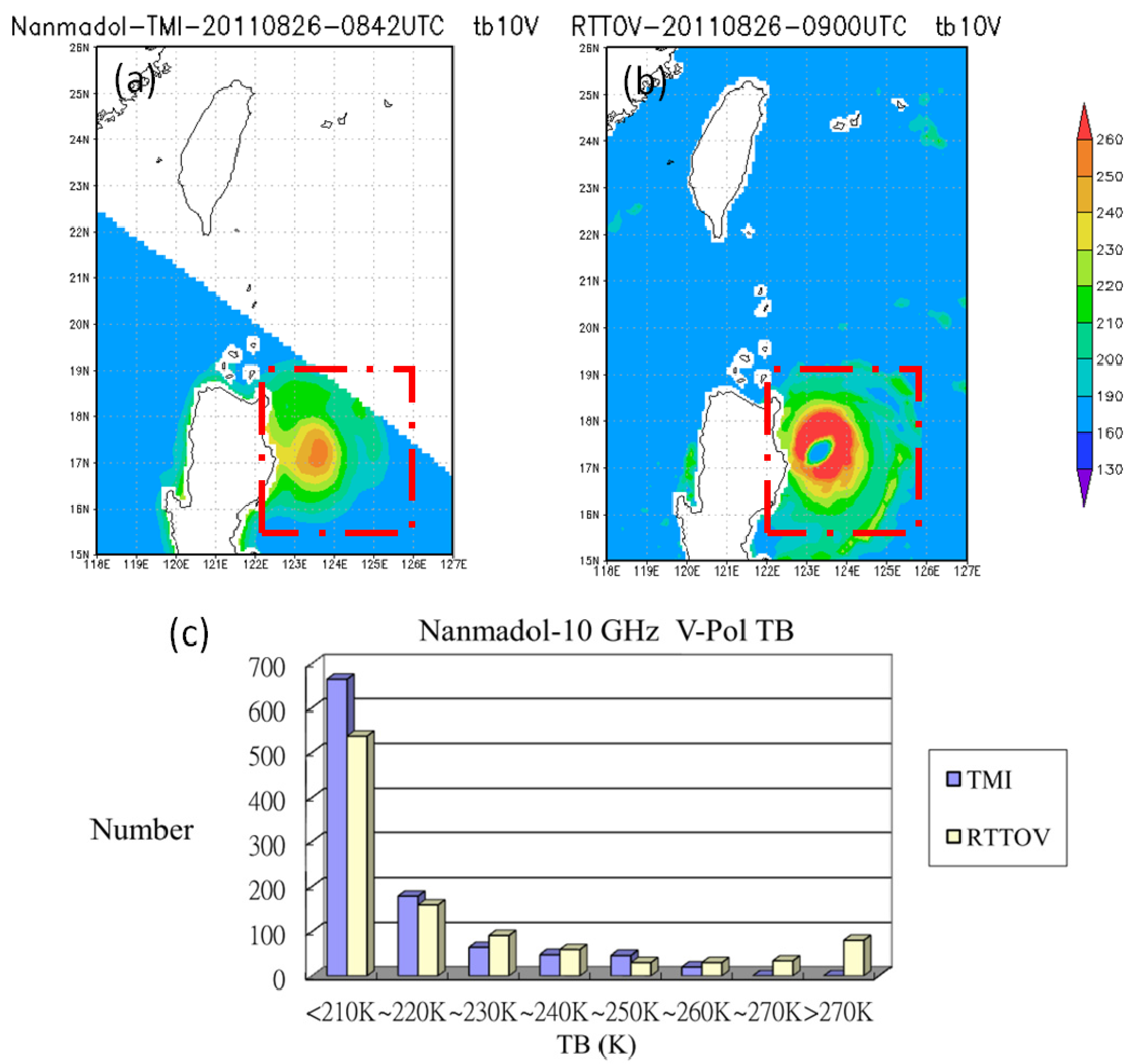
| 10-V GHz | 175.78 K | 1.27 K |
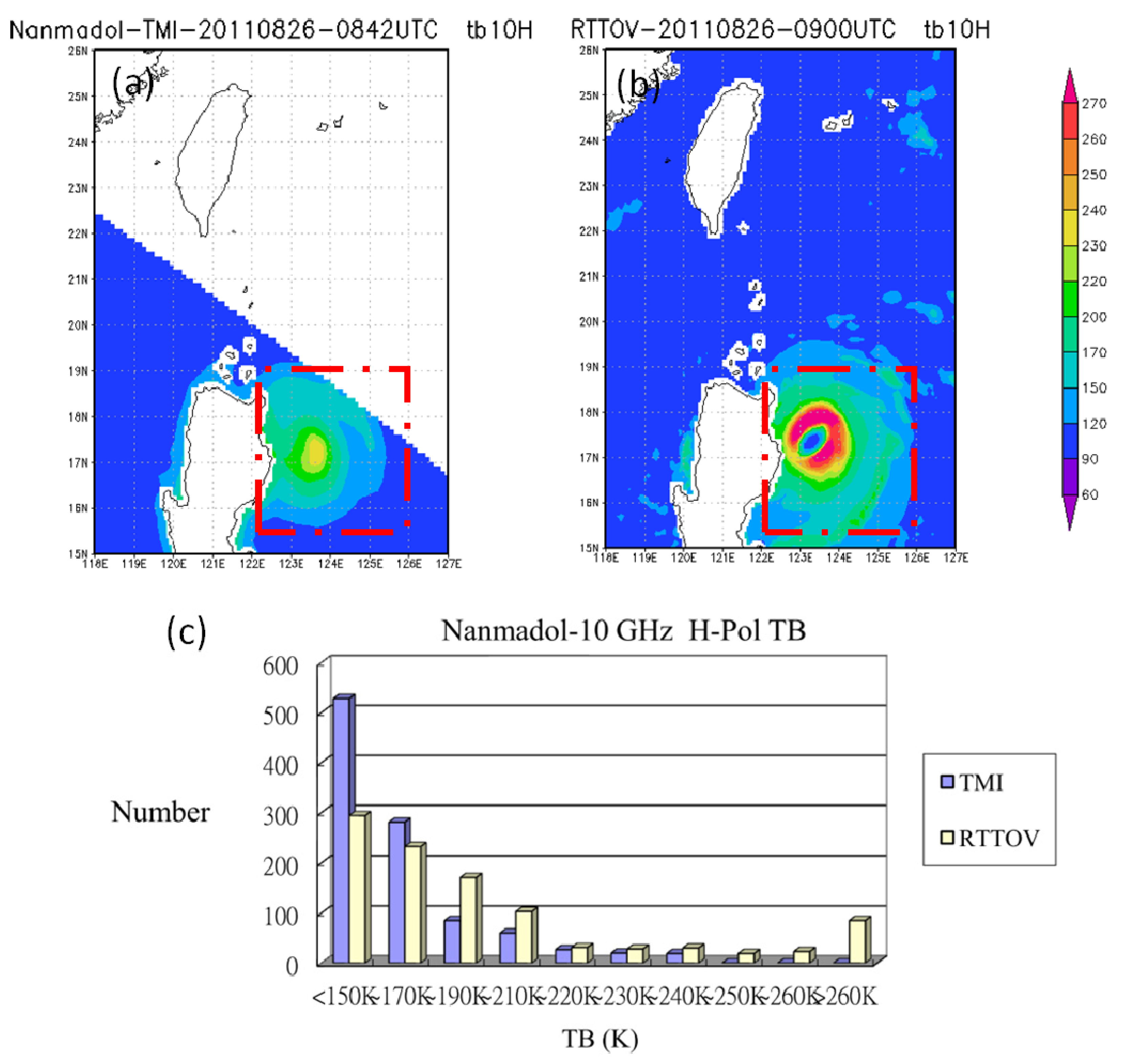
| 10-H GHz | 93.78 K | 2.39 K |
| 19-V GHz | 218.77 K | 2.73 K |
| 19-H GHz | 163.46 K | 5.05 K |
| 21-V GHz | 248.21 K | 3.41 K |
| 37-V GHz | 228.09 K | 2.39 K |
| 37-H GHz | 175.74 K | 5.05 K |
| 85-V GHz | 276.17 K | 1.63 K |
| 85-H GHz | 260.77 K | 3.76 K |
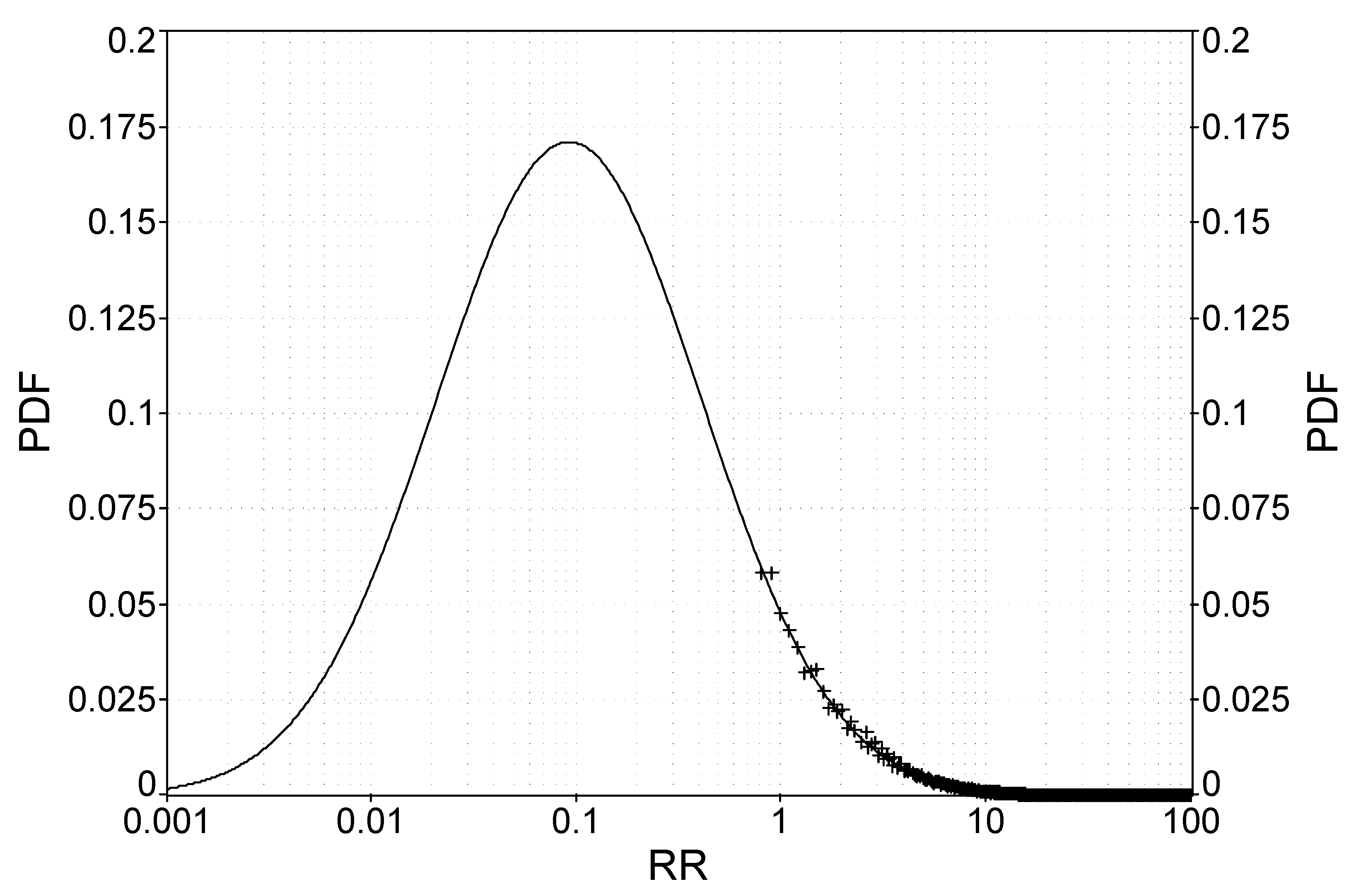
3.3. Prior PDF
3.4. Conditional PDF
| Number | Typhoon Nane | Typhoon Strength | Simulation Time (UTC) |
|---|---|---|---|
| 1 | BOLAVEN | Strong | 2012/8/25 1800–2012/8/26 1800 |
| 2 | GUCHOL | Strong | 2012/6/17 0600–2012/6/17 0600 |
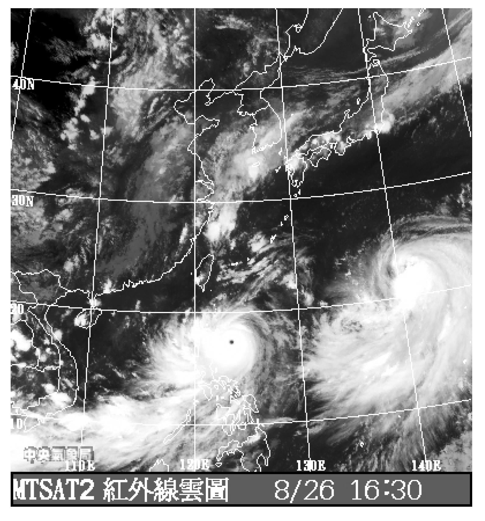
| 3 | NANMADOL | Strong | 2011/8/25 1800–2011/8/26 1800 |
| 4 | SONGDA | Strong | 2011/5/26 1200–2011/5/27 1200 |
| 5 | SINLAKU | Strong | 2008/9/12 0600–2008/9/13 0600 |
| 6 | PRAPIROON | Medium | 2012/10/11 1800–2012/10/12 1800 |
| 7 | JELAWAT | Medium | 2012/9/28 0000–2012/9/29 0000 |
| 8 | SANBA | Medium | 2012/9/14 1200–2012/9/15 1200 |
| 9 | HAIKUI | Medium | 2012/8/6 0000–2012/8/7 0000 |
| 10 | MUIFA | Medium | 2011/8/3 0600–2011/8/4 0600 |
| 11 | CHABA | Medium | 2010/10/27 1800–2010/10/28 1800 |
| 12 | MEGI | Medium | 2010/10/21 0000–2010/10/22 0000 |
| 13 | FANAPI | Medium | 2010/9/17 1200–2010/9/18 1200 |
| 14 | LUPIT | Medium | 2009/10/18 0000–2009/10/19 0000 |
| 15 | PARMA | Weak | 2009/10/4 0600–2009/10/5 0600 |
3.5. Posterior PDF
4. Validation and Discussion
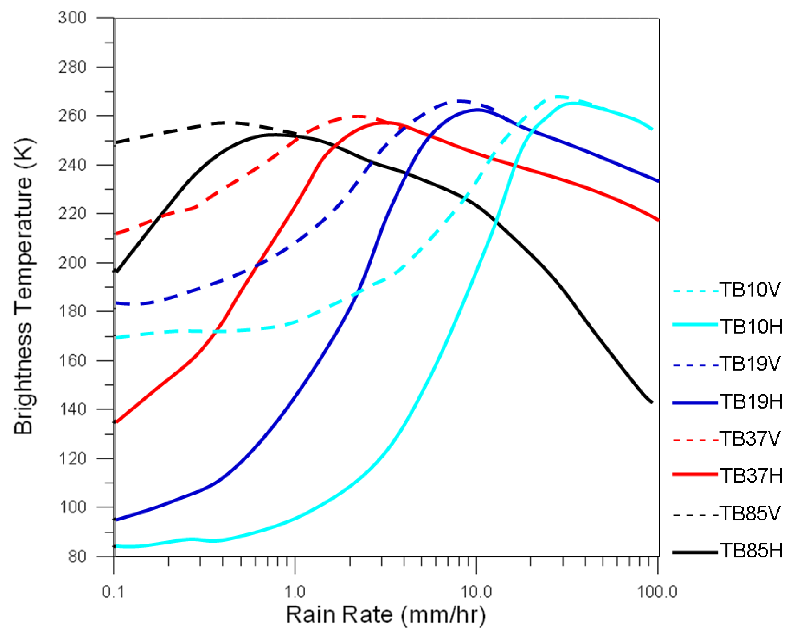
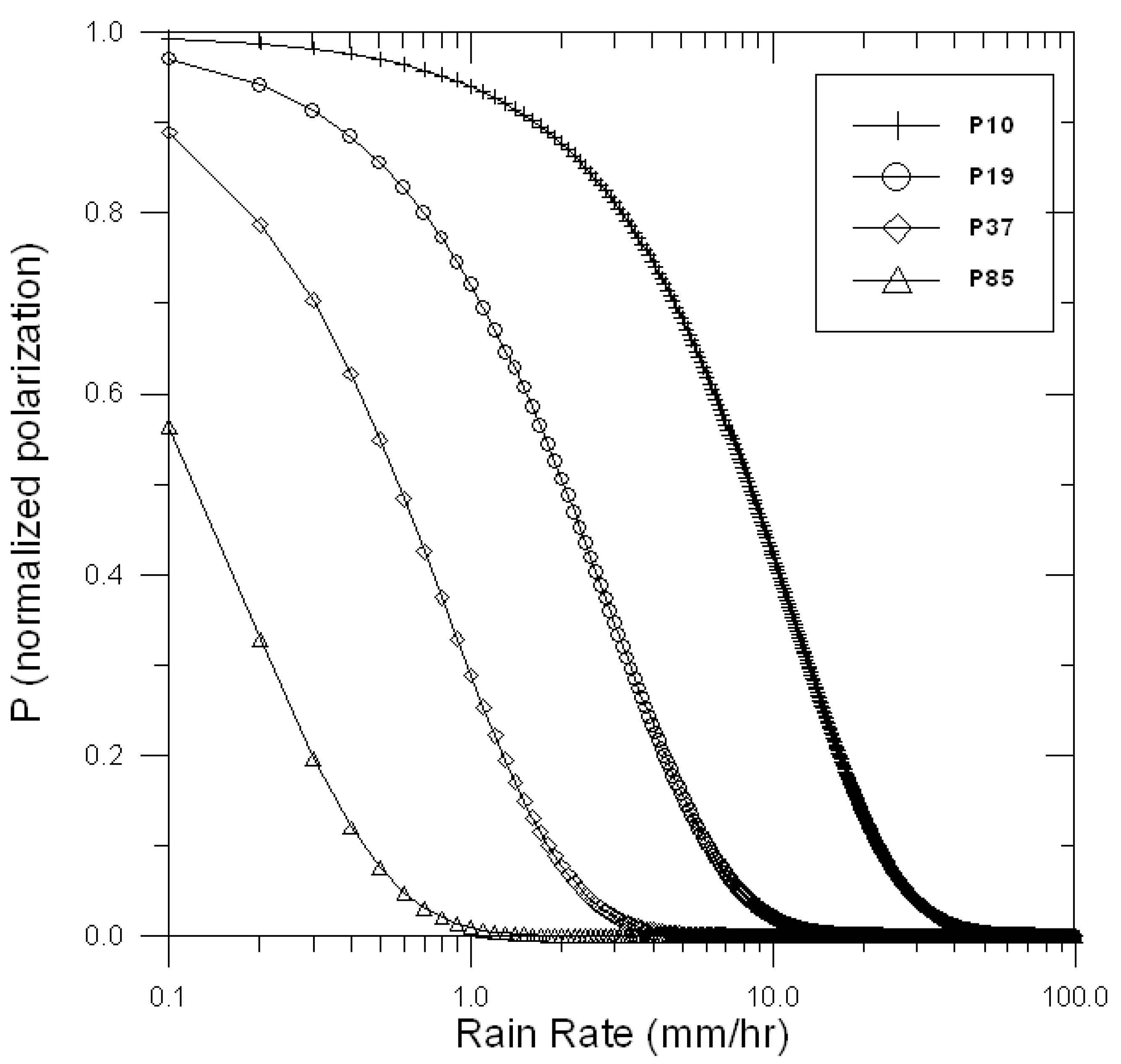
4.1. Analysis of TB
| No. | Typhoon Name | Scan Time (UTC) | The Range of Quantitative Analysis | Data Number | Correlation Coefficient | ||||
|---|---|---|---|---|---|---|---|---|---|
| North Latitude | East Longitude | ||||||||
| 1 | BOLAVEN | 2012/8/26 | 759 | 23 | 29 | 125 | 133 | 3437 | 0.74 |
| 2 | GUCHOL | 2012/6/17 | 1848 | 19.5 | 24 | 125 | 130 | 1846 | 0.87 |
| 3 | NANMADOL | 2011/8/26 | 842 | 15.5 | 19 | 122 | 126 | 1020 | 0.64 |
| 4 | SONGDA | 2011/5/27 | 609 | 17 | 22.5 | 121.5 | 126 | 1921 | 0.73 |
| 5 | SINLAKU | 2008/9/12 | 1912 | 22 | 26.5 | 121.5 | 125.5 | 1297 | 0.79 |
| 6 | PRAPIROON | 2012/10/12 | 709 | 17 | 23 | 126 | 132 | 3117 | 0.78 |
| 7 | JELAWAT | 2012/9/28 | 1508 | 23 | 28 | 123 | 128 | 1960 | 0.83 |
| 8 | SANBA | 2012/9/15 | 347 | 21.5 | 26 | 126 | 131 | 1840 | 0.8 |
| 9 | HAIKUI | 2012/8/6 | 1820 | 24 | 30 | 121.5 | 128 | 2589 | 0.7 |
| 10 | MUIFA | 2011/8/3 | 1841 | 21.5 | 27 | 128 | 134 | 2682 | 0.77 |
| 11 | CHABA | 2010/10/28 | 1016 | 23 | 28 | 127 | 131 | 1553 | 0.88 |
| 12 | MEGI | 2010/10/21 | 1330 | 21.5 | 27 | 128 | 134 | 2156 | 0.84 |
| 13 | FANAPI | 2010/9/18 | 620 | 21.5 | 25.5 | 123 | 128 | 1575 | 0.84 |
| 14 | LUPIT | 2009/10/18 | 1434 | 15 | 21 | 131 | 137 | 2307 | 0.82 |
| 15 | PARMA | 2009/10/4 | 2232 | 17 | 22 | 117 | 122 | 1691 | 0.72 |
Validation of TB Simulation


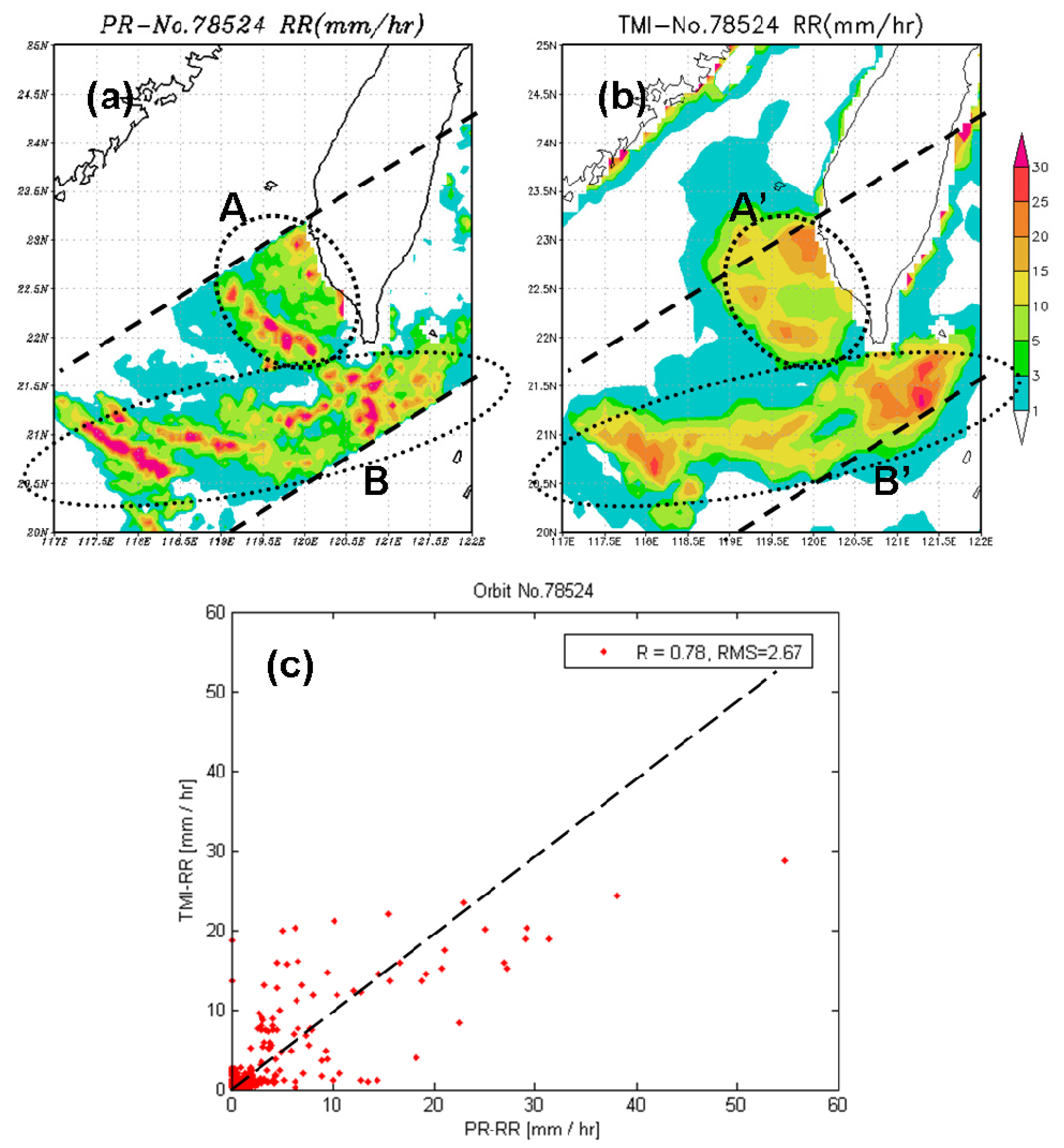
4.2. Validation of RR Estimation
| Number | Typhoon Name | Scan Time (UTC) | Orbital Number | Correlation Coefficient | RMSE |
|---|---|---|---|---|---|
| 1 | MUIFA | 2011/08/03 1307 | 78127 | – | – |
| 2 | MUIFA | 2011/08/03 1940 | 78131 | 0.52 | 3.48 |
| 3 | MUIFA | 2011/08/04 1732 | 78146 | – | – |
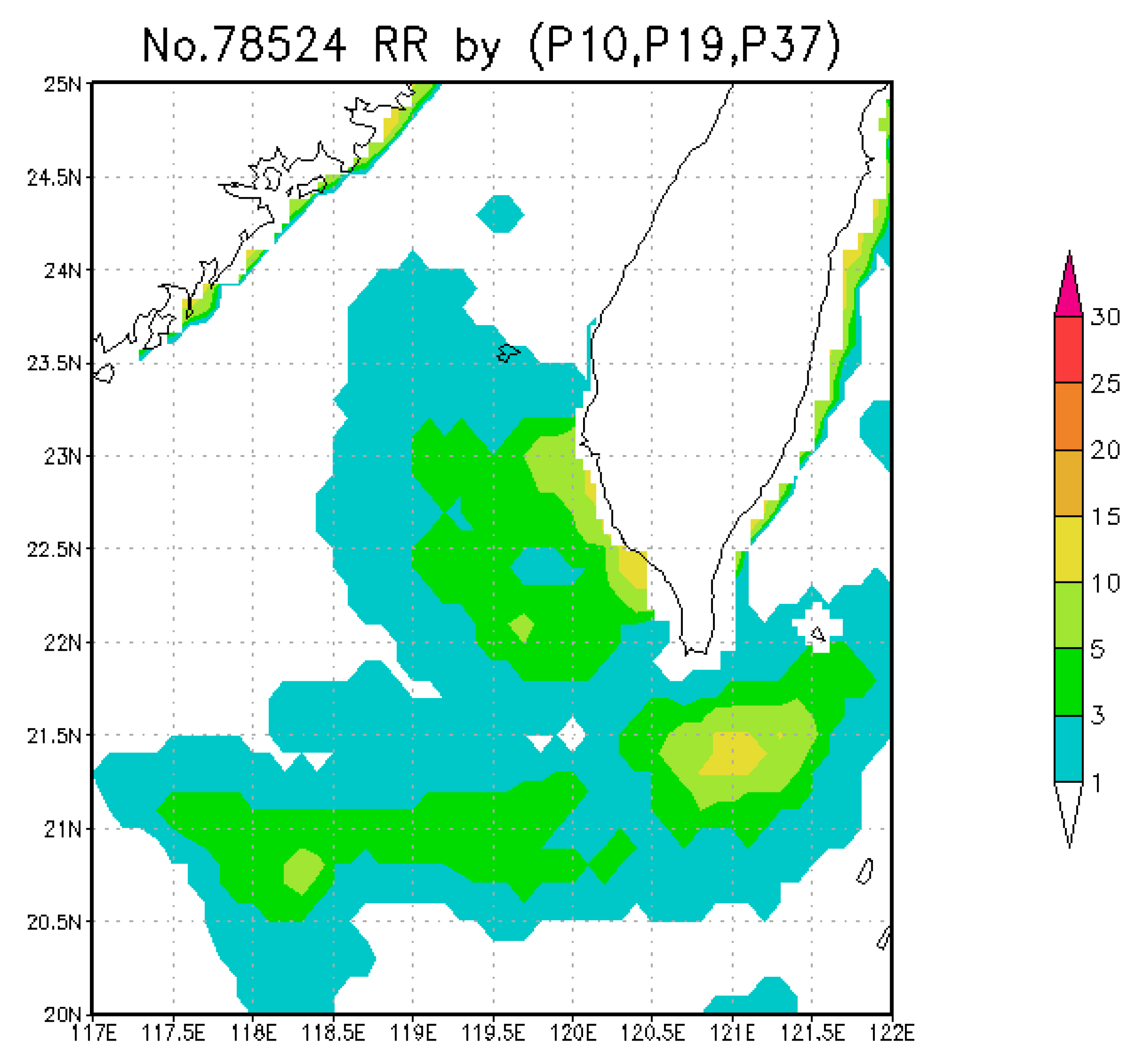
| 4 | NANMADOL | 2011/08/29 0025 | 78524 | 0.78 | 2.67 |
| 5 | TEMBIN | 2012/08/23 0943 | 84141 | 0.7 | 4.63 |
| 6 | TEMBIN | 2012/08/26 0832 | 84187 | 0.58 | 4.27 |
| 7 | TEMBIN | 2012/08/27 0736 | 84202 | 0.54 | 2.36 |
| 8 | SANBA | 2012/09/12 0733 | 84451 | 0.44 | 6.05 |
| 9 | SANBA | 2012/09/14 0540 | 84481 | 0.66 | 5.97 |
| 10 | JELAWAT | 2012/09/28 1544 | 84706 | 0.72 | 6.14 |
Case Study


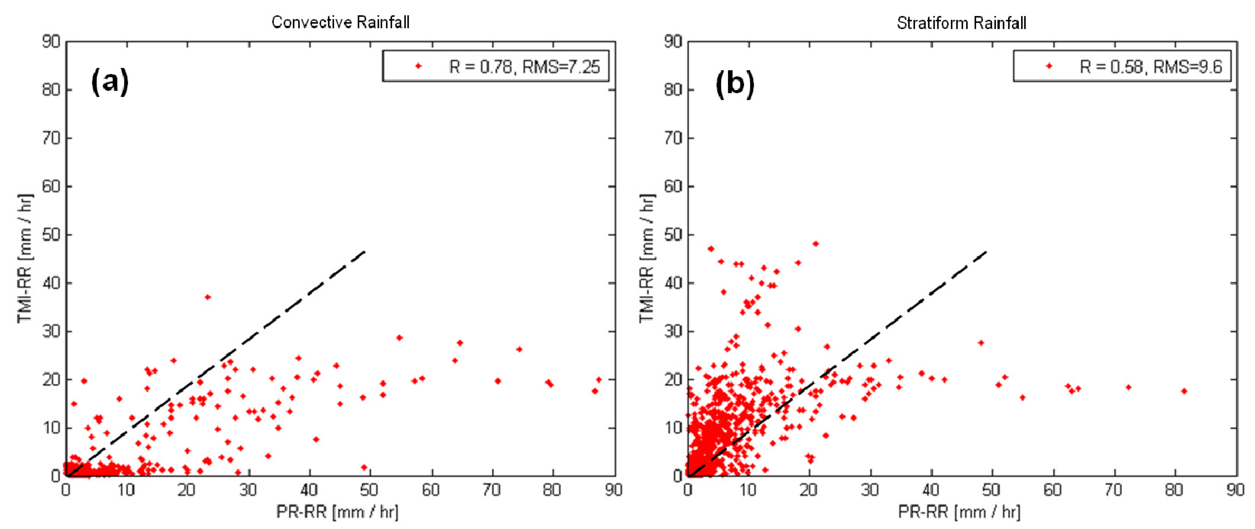
4.3. Precipitation Type Analysis

5. Conclusions
Acknowledgments
Author Contributions
Conflicts of Interest
References
- Adler, R.F.; Rodgers, E.B. Satellite-observed latent heat release in tropical cyclones. Mon. Weather Rev. 1997, 105, 956–963. [Google Scholar] [CrossRef]
- Spencer, R.W.; Hinton, B.B.; Olson, W.S. Nimbus-7 37 GHz radiances correlated with radar rain rates over the Gulf of Mexico. J. Climate Appl. Meteorol. 1983, 22, 2095–2099. [Google Scholar] [CrossRef]
- Wilheit, T.T. Algorithm for the retrieval of rainfall from passive microwave measurements. Remote Sens. Rev. 1994, 11, 163–194. [Google Scholar] [CrossRef]
- Barrett, E.C. The first WetNet precipitation intercomparison project (PIP-1): Interpretation of results. Remote Sens. Rev. 1994, 11, 303–373. [Google Scholar] [CrossRef]
- Petty, G.W. The status of satellite-based rainfall estimation over land. Remote Sens. Environ. 1995, 51, 125–137. [Google Scholar] [CrossRef]
- Smith, E.A.; Lamm, J.E.; Adler, R.; Alishouse, J.; Aonashi, K.; Barrett, E.; Bauer, P.; Berg, W.; Chang, A.; Ferraro, R.; et al. Results of WetNet PIP-2 project. J. Atmos. Sci. 1998, 55, 1483–1536. [Google Scholar] [CrossRef]
- Levizzani, V.; Amorati, R.; Meneguzzo, F. A Review of Satellite-based Rainfall Estimation Methods; European Commission Project Music Report: Brussels, Belgium, 2002; pp. 1–66. [Google Scholar]
- Kidd, C.; Kniveton, D.R.; Todd, M.C.; Bellerby, T.J. Satellite Rainfall Estimation Using a Combined Passive Microwave and Infrared Algorithm. J. Hydrometeorol. 2003, 4, 1088–1104. [Google Scholar] [CrossRef]
- Adler, R.F.; Kidd, C.; Petty, G.; Morissey, M.; Goodman, H.M. Intercomparison of global precipitation products: The third precipitation interconparison project (PIP-3). Bull. Am. Meteorol. Soc. 2001, 82, 1377–1396. [Google Scholar] [CrossRef]
- Petty, G.W. Physical Retrievals of Over-Ocean Rain Rate from Multichannel Microwave Imagery. Part I: Theoretical Characteristics of Normalized Polarization and Scattering Indices. Meteorol. Atmos. Phys. 1994, 54, 79–100. [Google Scholar] [CrossRef]
- Chen, W.J.; Li, C.C. Rain Retrievals Using Tropical Rainfall Measuring Mission and Geostationary Meteorological Satellite 5 Data Obtained during the SCSMEX. Int. J. Remote Sens. 2002, 23, 2425–2448. [Google Scholar] [CrossRef]
- Liu, G.R.; Liu, C.C.; Kuo, T.H. A Satellite-Derived Objective Potential Index for MCS Development during the Mei-Yu Period. J. Meteorol. Soc. Jpn. 2002, 80, 503–517. [Google Scholar] [CrossRef]
- Joyce, R.J.; Janowiak, J.E.; Arkin, P.A.; Xie, P. CMORPH: A Method that Produces Global Precipitation Estimates from Passive Microwave and Infrared Data at High Spatial and Temporal Resolution. J. Hydrometeorol. 2004, 5, 487–503. [Google Scholar] [CrossRef]
- Kummerow, C.; Shin, D.B.; Hong, Y.; Olson, W.S.; Yang, S.; Adler, R.F.; McCollum, J.; Ferraro, R.; Petty, G.; Wilheit, T.T. The Evolution of the Goddard Profiling Algorithm (GPROF) for Rainfall Estimation from Passive Microwave Sensors. J. Appl. Meteorol. 2001, 40, 1801–1820. [Google Scholar] [CrossRef]
- Arkin, P.A.; Meisner, B. The Relationship between Large-Scale Convective Rainfall and Cold Cloud over the Western Hemisphere during 1982–1984. Mon. Weather Rev. 1987, 115, 51–74. [Google Scholar] [CrossRef]
- Chiu, L.S.; North, G.R.; Short, D.A.; McConnell, A. Rain Estimation from Satellites: Effect of Finite Field of View. J. Geophys. Res. 1990, 95, 2177–2185. [Google Scholar] [CrossRef]
- Adler, R.F.; Negri, A.J.; Keehn, P.R.; Hakkarinen, I.M. Estimation of Monthly Rainfall over Japan and Surrounding Waters from a Combination of Low-Orbit Microwave and Geosynchronous IR Data. J. Appl. Meteorol. 1993, 32, 335–356. [Google Scholar] [CrossRef]
- Ferraro, R.R. SSM/I Derived Global Rainfall Estimates for Climatological Applications. J. Geophys. Res. 1997, 102, 16715–16735. [Google Scholar] [CrossRef]
- Wilheit, T.T.; Chang, A.T.C.; Chiu, L.S. Retrieval of Monthly Rainfall Indices from Microwave Radiometric Measurements Using Probability Distribution Functions. J. Atmos. Ocean. Technol. 1991, 8, 118–136. [Google Scholar] [CrossRef]
- Janowiak, J.E. Tropical Rainfall: A Comparison of Satellite-Derived Rainfall Estimates with Model Precipitation Forecasts, Climatologies, and Observations. Mon. Weather Rev. 1992, 120, 448–462. [Google Scholar] [CrossRef]
- Grody, N.C. Classification of Snow Cover and Precipitation Using the Special Sensor Microwave Imager. J. Geophys. Res. 1991, 96, 7423–7435. [Google Scholar] [CrossRef]
- Ferraro, R.R.; Grody, N.C.; Marks, G.F. Effects of Surface Conditions on Rain Identification Using the SSM/I. Remote Sens. Rev. 1994, 11, 195–209. [Google Scholar] [CrossRef]
- Ferraro, R.R.; Weng, F.; Grody, N.C.; Basist, A. An Eight-Year (1987–1994) Time Series of Rainfall, Clouds, Water Vapor, Snow Cover, and Sea Ice Derived from SSM/I Measurements. Bull. Am. Meteorol. Soc. 1996, 77, 891–905. [Google Scholar] [CrossRef]
- Kidder, S.Q.; VonderHaar, T.H. Satellite Meteorology: An Introduction; Academic Press: San Diego, CA, USA, 1995; pp. 1–339. [Google Scholar]
- Wilheit, T.; Kummerow, C.; Ferraro, R. Rainfall Algorithms for AMSR-E. IEEE Trans. Geosci. Remote Sens. 2003, 41, 204–214. [Google Scholar] [CrossRef]
- Kidd, C.; Huffman, G. Global precipitation measurement. Meteorol. Appl. 2011, 18, 334–353. [Google Scholar] [CrossRef]
- Tapiador, F.J.; Turk, J.; Petersen, W.; Hou, A.Y.; García-Ortega, E.; Machado, L.A.T.; Angelis, C.F.; Salio, P.; Kidd, C.; Huffman, G.J. Global precipitation measurement: Methods, datasets and applications. Atmos. Res. 2012, 104–105, 70–97. [Google Scholar] [CrossRef]
- Chen, S.; Hong, Y.; Gourley, J.J.; Kirstette, P.E.; Yong, B.; Tian, Y.; Zhang, Z.; Hardy, J. Similarity and difference of the two successive V6 and V7 TRMM multi-satellite precipitation analysis (TMPA) performance over China. J. Geophys. Res. 2013, 118, 13060–13074. [Google Scholar]
- Chen, S.; Hong, Y.; Gourley, J.J.; Huffman, G.J.; Tian, Y.; Cao, Q.; Kirstetter, P.E.; Hu, J.; Hardy, J.; Xue, X. Evaluation of the successive V6 and V7 TRMM multi-satellite precipitation analysis over the continental United States. Water Resour. Res. 2013, 49, 8174–8186. [Google Scholar] [CrossRef]
- Kirstetter, P.E.; Hong, Y.; Gourley, J.; Schwaller, M.; Petersen, W.; Zhang, J. Comparison of TRMM 2A25 products, version 6 and version 7, with NOAA/NSSL ground radar-based national mosaic QPE. J. Hydrometeorol. 2013, 14, 661–669. [Google Scholar] [CrossRef]
- Huang, Y.; Chen, S.; Cao, Q.; Hong, Y.; Wu, B.; Huang, M.; Qiao, L.; Zhang, Z.; Li, Z.; Li, W.; Yang, X. Evaluation of Version-7 TRMM Multi-Satellite Precipitation Analysis Product during the Beijing Extreme Heavy Rainfall Event of 21 July 2012. Water 2014, 6, 32–44. [Google Scholar] [CrossRef]
- Rana, S.; McGregor, J.; Renwick, J.A. Precipitation seasonality over the Indian Subcontinent: An evaluation of gauge, reanalyses and satellite retrievals. J. Hydrometeorol. 2015, 16, 631–651. [Google Scholar] [CrossRef]
- Chau, K.W.; Wu, C.L. A Hybrid Model Coupled with Singular Spectrum Analysis for Daily Rainfall Prediction. J. Hydroinform. 2010, 12, 458–473. [Google Scholar] [CrossRef]
- Wang, W.C.; Chau, K.W.; Xu, D.M.; Chen, X.Y. Improving forecasting accuracy of annual runoff time series using ARIMA based on EEMD decomposition. Water Resour. Manag. 2015, 29, 2655–2675. [Google Scholar] [CrossRef]
- Hu, J.C.; Chen, W.J.; Chiu, J.C.; Wang, J.L.; Liu, G.R. Quantitative Precipitation Estimation over Ocean Using Bayesian Approach from Microwave Observations during the Typhoon Season. Terr. Atmos. Ocean. Sci. 2009, 20, 817–832. [Google Scholar] [CrossRef]
- Petty, G.W.; Boukabara, S.A.; Snell, N.; Moncet, J.L. Algorithm Theoretical Basis Document (ATBD) for the Conical-Scanning Microwave Imager/Sounder (CMIS) Environmental Data Records (EDRs), Volume 5: Precipitation Type and Rate EDR; Atmospheric and Environmental Research: Lexington, MA, USA, 2001; pp. 1–112. [Google Scholar]
- Chiu, J.C. Bayesian Retrieval of Complete Posterior PDFs of Rain Rate from Satellite Passive Microwave Observations. Ph.D. Thesis, Purdue University, West Lafayette, IN, USA, 2003. [Google Scholar]
- Chiu, J.C.; Petty, G.W. Bayesian Retrieval of Complete Posterior PDFs of Oceanic Rain Rate from Microwave Observations. J. Appl. Meteorol. Climatol. 2006, 45, 1073–1095. [Google Scholar] [CrossRef]
- Okamoto, K. Tropical Rainfall Measuring Mission (TRMM) Precipitation Radar Algorithm Instruction Manual for Version 6. TRMM Precipitation Radar Team. Available online: http://www.eorc.jaxa.jp/TRMM/documents/PR_algorithm_product_information/pr_manual/PR_Instruction_Manual_V7_L1.pdf (accessed on 27 October 2015).
- Yeh, N.C.; Chen, W.J.; Wei, C.H.; Liu, C.Y. The Analysis of Hydrometeor Sensitivity on TRMM/TMI. J. Aeronaut. Astronaut. Aviat. 2014, 46, 203–207. [Google Scholar]
- Chien, F.C.; Hong, J.S.; Chang, W.J.; Jou, J.D.; Lin, P.L.; Lin, T.E.; Liu, S.P.; Miou, H.J.; Chen, C.Y. A Sensitivity Study of the WRF Model Part II: Verification of Quantitative Precipitation Forecasts. Atmos. Sci. 2006, 34, 261–276. (In Chinese) [Google Scholar]
- Iguchi, T.; Kozu, T.; Meneghini, R.; Awaka, J.; Okamoto, K. Rain-profiling algorithm for the TRMM precipitation radar. J. Appl. Meteorol. 2000, 39, 2038–2052. [Google Scholar] [CrossRef]
© 2015 by the authors; licensee MDPI, Basel, Switzerland. This article is an open access article distributed under the terms and conditions of the Creative Commons Attribution license (http://creativecommons.org/licenses/by/4.0/).
Share and Cite
Yeh, N.-C.; Liu, C.-C.; Chen, W.-J. Estimation of Rainfall Associated with Typhoons over the Ocean Using TRMM/TMI and Numerical Models. Water 2015, 7, 6017-6038. https://doi.org/10.3390/w7116017
Yeh N-C, Liu C-C, Chen W-J. Estimation of Rainfall Associated with Typhoons over the Ocean Using TRMM/TMI and Numerical Models. Water. 2015; 7(11):6017-6038. https://doi.org/10.3390/w7116017
Chicago/Turabian StyleYeh, Nan-Ching, Chung-Chih Liu, and Wann-Jin Chen. 2015. "Estimation of Rainfall Associated with Typhoons over the Ocean Using TRMM/TMI and Numerical Models" Water 7, no. 11: 6017-6038. https://doi.org/10.3390/w7116017