
Validation of a Locally Revised Topographic Index in Central New Jersey, USA

Abstract
:1. Introduction
2. Data and Methods
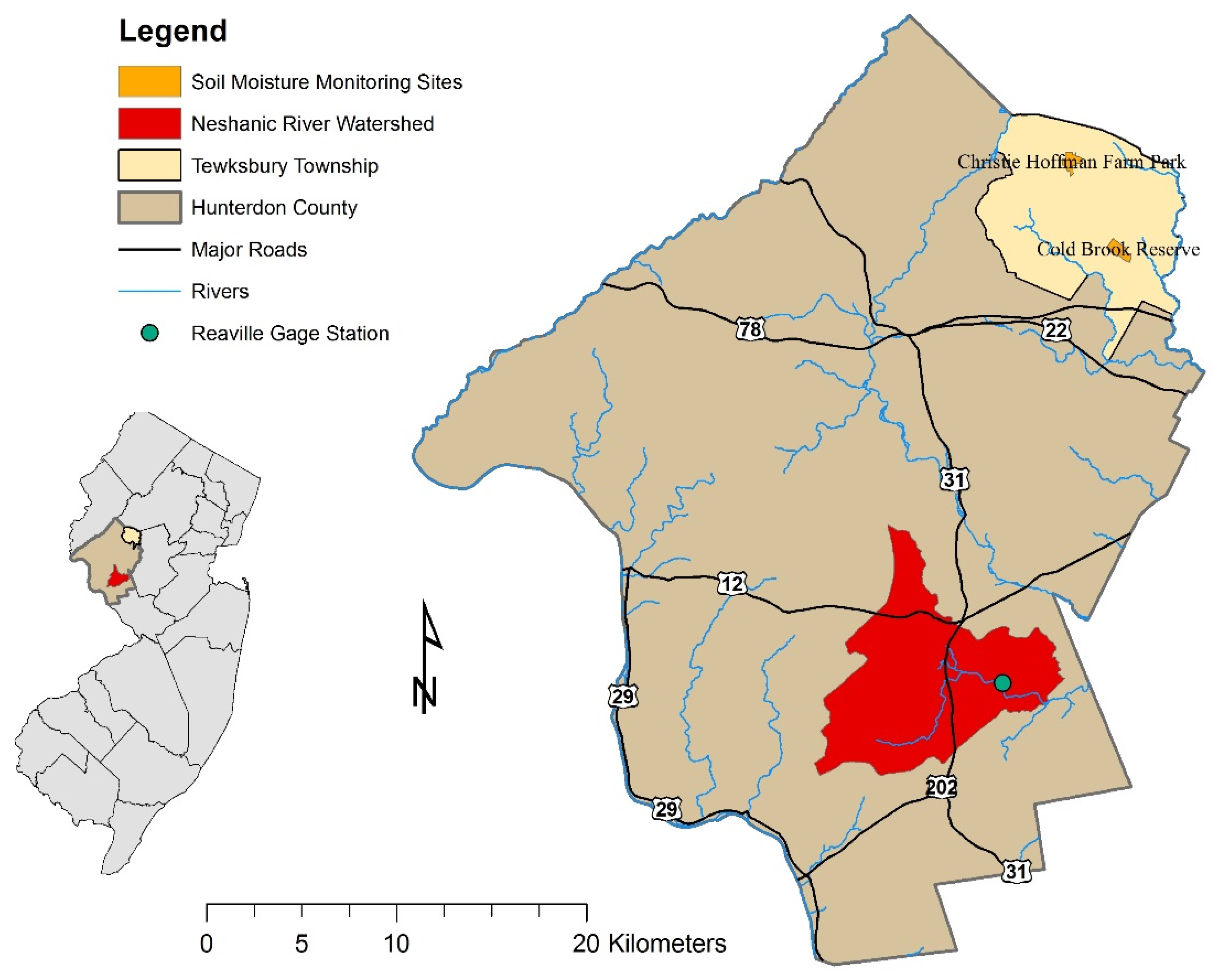
2.1. Study Area

2.2. Topographic Index
2.3. Soil Moisture Measurement

| Items | Sampling Site and Event | |||||
|---|---|---|---|---|---|---|
| Sampling Location | Cold Brook Farm | Christy Hoffman Park | ||||
| Sampling Date | 8 June 2009 | 1 December 2009 | 30 April 2010 | 1 December 2009 | 17 December 2009 | |
| Weather Conditions | Sunny, 78 °F, no rain in past two days | Sunny, windy, 47 °F; 0.86 cm rain a day before | Sunny, 60 °F; 0.03 cm rain a day before | Sunny, windy, 47 °F; 0.86 cm rain a day before | Sunny, windy, 29 °F; no rain a day before | |
| Sampling Points | 146 | 138 | 140 | 111 | 158 | |
| TDR Reading | Mean | 19.5 | 5.6 | 25.3 | 7.4 | 15.2 |
| Minimum | 11.6 | 2.3 | 14 | 2.9 | 2.6 | |
| Maximum | 39.4 | 9.5 | 37.9 | 11.8 | 31.5 | |
| Corresponding Topographic Index | Mean | 7.5 | 7.5 | 8.1 | 7.6 | 8.3 |
| Minimum | 5.9 | 6.3 | 5.9 | 5.3 | 5.2 | |
| Maximum | 10.4 | 9.1 | 12.4 | 12.3 | 12.0 | |
2.4. VSLF Modeling

2.5. SWAT Modeling
3. Results
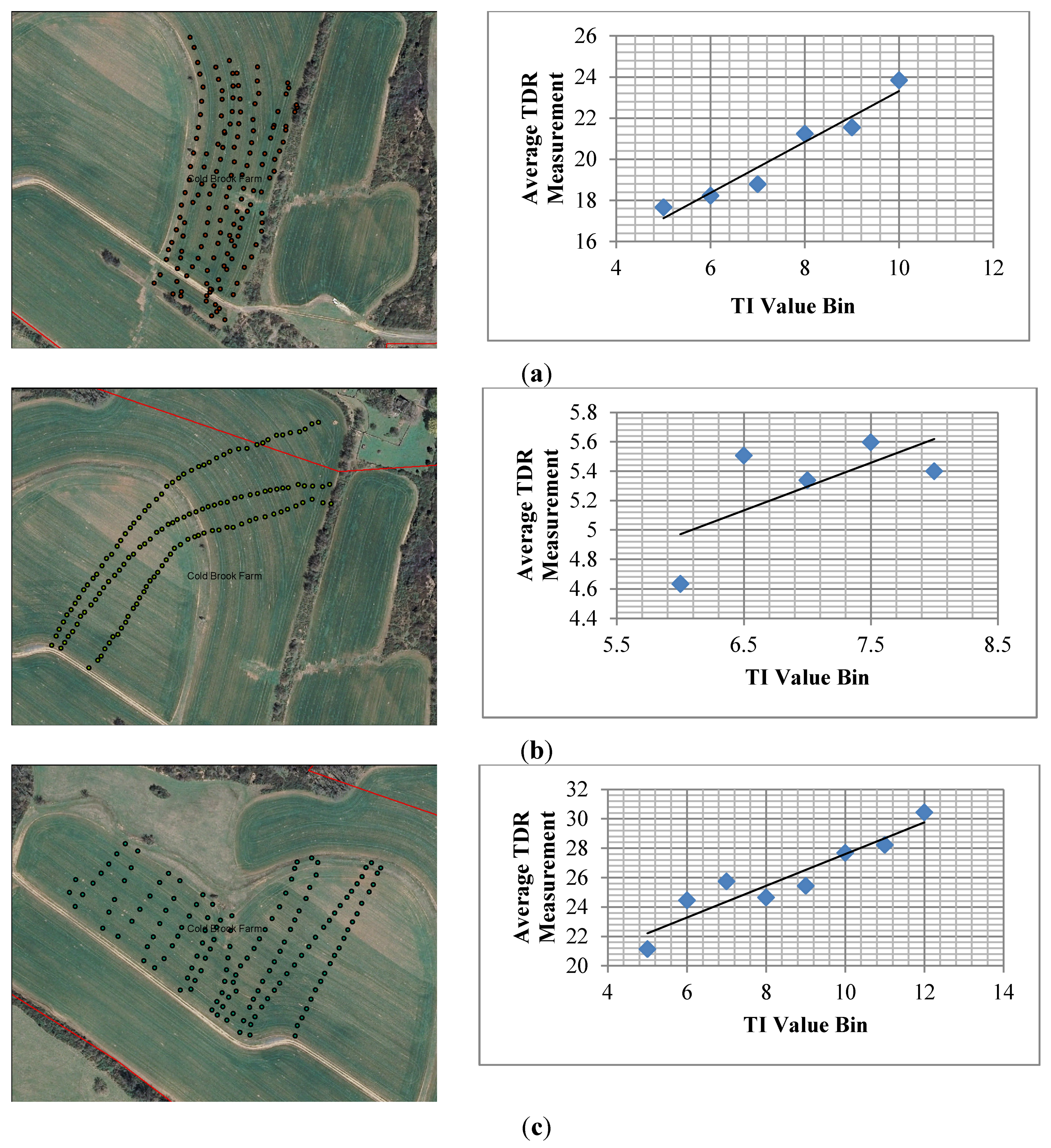
3.1. Comparison between DTR Measurements and TI Values


3.2. Comparison between VSLF and SWAT
| Hydrology Calibration Parameter | Affected Output Variable | Optimization Goal | Default Value | Original Value | Calibrated Value |
|---|---|---|---|---|---|
| Precip. Correction Factor | Stream flow | Minimize bias | 1 | 0.951625 | 0.950230 |
| SMIN Factor | Runoff per [day dormant] | Minimize bias | 0.434783 | 0.170942 | 0.183991 |
| SMAX Factor | Runoff per [day growing] | Minimize bias | 2.380950 | 1.343430 | 1.190920 |
| Runoff Recess Coefficient | Runoff | Maximize NSE | 1 | 0.412917 | 0.901439 |
| Melt Factor | Stream flow | Maximize NSE | 0.45 | 0.409741 | 0.992740 |
| Recess Coefficient | Base flow | Maximize NSE | 0.1 | 0.061885 | 0.095339 |
| Bypass Coefficient | Stream flow (lowflow) | Minimize bias | 0 | 0.059946 | 0.028769 |
| Flow | Time Period | Mean (cm/day) | Standard Deviation (cm/day) | NSE | |||||
|---|---|---|---|---|---|---|---|---|---|
| USGS | SWAT | VSLF | USGS | SWAT | VSLF | SWAT | VSLF | ||
| Surface runoff | Annual | 34.98 | 23.83 | 33.22 | 20.11 | 5.77 | 13.15 | 0.48 | 0.85 |
| Monthly | 2.32 | 1.99 | 2.48 | 3.98 | 2.18 | 2.75 | 0.65 | 0.68 | |
| Daily | 0.07 | 0.07 | 0.08 | 0.59 | 0.31 | 0.35 | 0.58 | 0.54 | |
| Baseflow | Annual | 25.84 | 20.25 | 25.76 | 9.69 | 3.09 | 7.07 | −1.95 | 0.64 |
| Monthly | 1.84 | 1.68 | 2.06 | 1.79 | 1.16 | 1.98 | 0.61 | 0.75 | |
| Daily | 0.06 | 0.06 | 0.07 | 0.07 | 0.06 | 0.07 | 0.37 | 0.55 | |
| Streamflow | Annual | 60.82 | 44.09 | 58.98 | 28.78 | 8.23 | 20.07 | 0.40 | 0.86 |
| Monthly | 4.15 | 3.67 | 4.54 | 5.20 | 3.11 | 4.43 | 0.68 | 0.74 | |
| Daily | 0.13 | 0.12 | 0.15 | 0.62 | 0.34 | 0.38 | 0.57 | 0.54 | |
| Flow | Time Period | Mean (cm/day) | Standard Deviation (cm/day) | NSE | |||||
|---|---|---|---|---|---|---|---|---|---|
| USGS | SWAT | VSLF | USGS | SWAT | VSLF | SWAT | VSLF | ||
| Surface runoff | Annual | 35.28 | 32.63 | 41.29 | 8.28 | 3.52 | 6.60 | 0.52 | 0.38 |
| Monthly | 3.04 | 2.73 | 3.50 | 3.26 | 2.50 | 3.33 | 0.63 | 0.81 | |
| Daily | 0.10 | 0.09 | 0.12 | 0.44 | 0.34 | 0.46 | 0.33 | 0.30 | |
| Baseflow | Annual | 28.42 | 30.30 | 32.47 | 6.62 | 4.61 | 3.24 | 0.72 | 0.14 |
| Monthly | 2.49 | 2.63 | 2.73 | 1.87 | 1.49 | 2.23 | 0.71 | 0.59 | |
| Daily | 0.08 | 0.09 | 0.09 | 0.09 | 0.08 | 0.09 | 0.50 | 0.55 | |
| Streamflow | Annual | 63.71 | 62.93 | 73.76 | 13.96 | 7.90 | 9.44 | 0.75 | 0.35 |
| Monthly | 5.53 | 5.35 | 6.23 | 4.85 | 3.60 | 4.98 | 0.68 | 0.79 | |
| Daily | 0.18 | 0.18 | 0.21 | 0.48 | 0.37 | 0.50 | 0.37 | 0.38 | |

4. Conclusions
Acknowledgments
Conflicts of Interest
References
- Steenhuis, T.S.; Muck, R.E. Preferred movement of nonadsorbed chemicals on wet, shallow, sloping, soils. J. Environ. Qual. 1988, 17, 376–384. [Google Scholar] [CrossRef]
- Merwin, I.A.; Stiles, W.C.; Vanes, H.M. Orchard groundcover management impacts on soil physical-properties. J. Am. Soc. Hort. Sci. 1994, 119, 216–222. [Google Scholar]
- Walter, M.T.; Mehta, V.K.; Marrone, A.M.; Boll, J.; Gérard-Merchant, P.; Steenhuis, T.S.; Walter, M.F. A simple estimation of the prevalence of Hortonian flow in New York City’s watersheds. J. Hydrol. Eng. 2003, 8, 214–218. [Google Scholar] [CrossRef]
- Hewlett, J.D.; Hibbert, A.R. Factors affecting the response of small watersheds to precipitation in humid areas. In Forest Hydrology; Sopper, W.E., Lull, H.W., Eds.; Pergamon Press: Oxford, UK, 1967; pp. 275–290. [Google Scholar]
- Dunne, T.; Leopold, L.B. Water in Environmental Planning; W.H. Freeman and Company: New York, NY, USA, 1978; p. 818. [Google Scholar]
- Hewlett, J.D. Principles of Forest Hydrology; University of Georgia Press: Athens, GA, USA, 1982; p. 183. [Google Scholar]
- Gburek, W.D.; Sharpley, A.N. Hydrologic controls on phosphorus loss from upland agricultural watersheds. J. Environ. Qual. 1998, 27, 267–277. [Google Scholar] [CrossRef]
- Walter, M.T.; Walter, M.F.; Brooks, E.S.; Steenhuis, T.S.; Boll, J.; Weiler, K. Hydrologically sensitive areas: Variable source area hydrology implications for water quality risk assessment. J. Soil Water Conserv. 2000, 55, 277–284. [Google Scholar]
- Walter, M.T.; Brooks, E.S.; Walter, M.F.; Steenhuis, T.S.; Scott, C.A.; Boll, J. Evaluation of soluble phosphorus loading from manure-applied fields under various spreading strategies. J. Soil Water Conserv. 2001, 56, 329–335. [Google Scholar]
- Heathwaite, L.; Quinn, P.F.; Hewett, C. Modelling and managing critical source areas of diffuse pollution from agricultural land using flow connectivity simulation. J. Hydrol. 2005, 304, 446–461. [Google Scholar] [CrossRef]
- Agnew, L.J.; Walter, M.T.; Lembo, A.; Gérard-Marchant, P.; Steenhuis, T.S. Identifying hydrologically sensitive areas: Bridging science and application. J. Environ. Manag. 2006, 78, 64–76. [Google Scholar] [CrossRef] [PubMed]
- Qiu, Z. Identifying critical source areas in watersheds for conservation buffer planning and riparian restoration. Environ. Manag. 2009, 44, 968–980. [Google Scholar] [CrossRef] [PubMed]
- Qiu, Z.; Hall, C.; Drewes, D.; Messinger, G.; Prato, T.; Hale, K.; van Abs, D. Hydrologically sensitive areas, municipal land use controls and protection of healthy watersheds. J. Water Res. Plan. Manag. 2014, 140. [Google Scholar] [CrossRef]
- Beven, K.J.; Kirkby, M.J. A physically based, variable contributing area model of basin hydrology. Hydrol. Sci. Bull. 1979, 24, 43–69. [Google Scholar] [CrossRef]
- O’Loughlin, E.M. Prediction of surface saturation zones in natural catchments by topographic analysis. Water Resour. Res. 1986, 22, 794–804. [Google Scholar] [CrossRef]
- Moore, I.D.; Grayson, R.B.; Ladson, A.R. Digital terrain modelling: A review of hydrological, geomorphological, and biological applications. Hydrol. Proc. 1991, 5, 3–30. [Google Scholar] [CrossRef]
- Beven, K. TOPMODEL: A critique. Hydrol. Proc. 1997, 11, 1069–1085. [Google Scholar] [CrossRef]
- Gomez-Plaza, A.; Martinez-Mena, M.; Albaladejo, J.; Castillo, V.M. Factors regulating spatial distribution of soil water content in small semiarid catchments. J. Hydrol. 2001, 253, 211–226. [Google Scholar] [CrossRef]
- Wilson, D.J.; Western, A.W.; Grayson, R.B. A terrain and data-based method for generating the spatial distribution of soil moisture. Adv. Water Resour. 2005, 28, 43–54. [Google Scholar] [CrossRef]
- Hornberger, G.M.; Beve, K.J.; Csby, B.J.; Sappington, D.E. Shenandoah watershed study: Calibration of a topography-based, variable contributing area hydroloigical model to a small forested catchment. Water Resour. Res. 1985, 21, 1841–1850. [Google Scholar] [CrossRef]
- Wood, E.F.; Sivapalan, M.; Beven, K.J. Similarity and scale in catchment storm response. Rev. Geophys. 1990, 28, 1–18. [Google Scholar] [CrossRef]
- Gallart, F.; Latron, J.; Llorens, P.; Beven, K. Using internal catchment information to reduce the uncertainty of discharge and baseflow predictions. Adv. Water Resour. 2007, 30, 808–823. [Google Scholar] [CrossRef]
- Schneiderman, E.M.; Steenhuis, T.S.; Thongs, D.J.; Easton, Z.M.; Zion, M.S.; Neal, A.L.; Mendoza, G.F.; Walter, M.T. Incorporating variable source area hydrology into Curve Number based watershed loading functions. Hydrol. Proc. 2007, 21, 3410–3430. [Google Scholar]
- Grayson, R.B.; Western, A.W. Towards areal estimation of soil water content from point measurements: Time and space stability of mean response. J. Hydrol. 1998, 207, 68–82. [Google Scholar] [CrossRef]
- Yeakley, J.A.; Swank, W.T.; Swift, L.W.; Hornberger, G.M.; Shugart, H.H. Soil moisture gradients and controls on a southern Appalachian hillslope from drought through recharge. Hydrol. Earth Syst. Sci. 1998, 2, 41–49. [Google Scholar] [CrossRef]
- Grayson, R.B.; Blöschl, G.; Western, A.W.; McMahon, T.A. Advances in the use of observed spatial patterns of catchment hydrological response. Adv. Water Resour. 2002, 25, 1313–1334. [Google Scholar] [CrossRef]
- Moore, I.D.; Thompson, J.C. Are water table variations in a shallow forest soil consistent with the TOPMODEL concept? Water Resour. Res. 1996, 32, 663–669. [Google Scholar] [CrossRef]
- Siebert, J.; Bishop, K.H.; Nyberg, L. A test of TOPMODEL’s ability to predict spatially distributed groundwater levels. Hydrol. Proc. 1997, 11, 1131–1144. [Google Scholar] [CrossRef]
- Rodhe, A.; Seibert, J. Wetland occurrence in relation to topography: A test of topographic indices as moisture indicators. Agric. Forest Meteorol. 1999, 98, 325–340. [Google Scholar] [CrossRef]
- Merot, P.; Squividant, H.; Aurousseau, P.; Hefting, M.; Burt, T.; Maitre, V.; Kruk, M.; Butturini, A.; Thenail, C.; Viaud, V. Testing a climato-topographic index for predicting wetlands distribution along an European climate gradient. Ecol. Model. 2003, 163, 51–71. [Google Scholar] [CrossRef]
- Nyberg, L. Spatial variability of soil water content in the covered catchment at Gardsjon, Sweden. Hydrol. Proc. 1996, 10, 89–103. [Google Scholar] [CrossRef]
- Chaplot, V.; Walter, C. Subsurface topography to enhance the prediction of the spatial distribution of soil wetness. Hydrol. Proc. 2003, 17, 2567–2580. [Google Scholar] [CrossRef]
- Bardossy, A.; Lehmann, W. Spatial distribution of soil moisture in a small catchment. Part 1: Geostatistical analysis. J. Hydrol. 1998, 206, 1–15. [Google Scholar] [CrossRef]
- Sulebak, J.R.; Tallaksen, L.M.; Erichsen, B. Estimation of areal soil moisture by use of terrain data. Geogr. Ann. 2000, 82, 89–105. [Google Scholar] [CrossRef]
- Pellenq, J.; Kalmab, J.; Bouleta, G.; Saulnierc, G.M.; Wooldridgeb, S.; Kerra, Y.; Chehbouni, A. A disaggregation scheme for soil moisture based on topography and soil depth. J. Hydrol. 2003, 276, 112–127. [Google Scholar] [CrossRef]
- Walter, M.T.; Steenhuis, T.S.; Mehta, V.K.; Thongs, D.; Zion, M.; Schneiderman, E. A refined conceptualization of TOPMODEL for shallow-subsurface flows. Hydrol. Proc. 2002, 16, 2041–2046. [Google Scholar] [CrossRef]
- Lyon, S.W.; Gérard-Marcant, P.; Walter, M.T.; Steenhuis, T.S. Using a topographic index to distribute variable source area runoff predicted with the SCS-curve number equation. Hydrol. Proc. 2004, 18, 2757–2771. [Google Scholar] [CrossRef]
- Frankenberger, J.R.; Brooks, E.S.; Walter, M.T.; Walter, M.F.; Steenhuis, T.S. A GIS-based variable source area hydrology model. Hydrol. Proc. 1999, 13, 805–822. [Google Scholar] [CrossRef]
- De Alwis, D.A.; Easton, Z.M.; Dahlke, H.E.; Philpot, W.D.; Steenhuis, T.S. Unsupervised classification of saturated areas using a time series of remotely sensed images. Hydrol. Earth Syst. Sci. 2007, 11, 1609–1620. [Google Scholar] [CrossRef]
- Haith, D.A.; Shoemaker, L.L. Generalized Watershed Loading Functions for stream flow nutrients. Water Resour. Bull. 1987, 23, 471–478. [Google Scholar] [CrossRef]
- Schneiderman, E.M.; Pierson, D.C.; Lounsbury, D.G.; Zion, M.S. Modeling the hydrochemistry of the Cannonsville Watershed with Generalized Watershed Loading Functions (GWLF). J. Amer. Water Resour. Assoc. 2002, 38, 1323–1347. [Google Scholar] [CrossRef]
- New Jersey Department of Environmental Protection (NJDEP). 2008 New Jersey Integrated Water Quality Monitoring and Assessment Report. Available online: http://www.nj.gov/dep/wms/bwqsa/2008_final_IR_complete.pdf (accessed on 1 October 2015).
- Qiu, Z. Comparative assessment of stormwater and nonpoint source pollution bet management practices in suburban watershed management. Water 2013, 5, 280–291. [Google Scholar] [CrossRef]
- Freeze, R.A.; Cherry, J.A. Groundwater; Prentice-Hall Inc.: Englewood Cliffs, NJ, USA, 1979; p. 604. [Google Scholar]
- Tarboton, D.G. Terrain Analysis Using Digital Elevation Models (TauDEM). Available online: http://hydrology.usu.edu/taudem/taudem5/index.html (accessed on 14 August 2015).
- Spectrum Technologies, Inc. Fieldscout TDR 300 Soil Moisture Meter Product Manual; Spectrum Technologies Inc.: Plainfield, IL, USA, 2009; p. 20. [Google Scholar]
- New Jersey Department of Environmental Protection (NJDEP). NJDEP GPS Data Collection Standards for GIS Data Development. Available online: http://www.nj.gov/dep/gis/GPSStandards_2011.pdf (accessed on 1 October 2015).
- New Jersey Department of Environmental Protection (NJDEP). 2002 Land Use/Land Cover by Watershed Management Area. Available online: http://www.state.nj.us/dep/gis/lulc02cshp.html (accessed on 1 October 2015).
- Nash, J.E.; Sutcliffe, J.V. River flow forecasting through conceptual models, part 1—A discussion of principles. J. Hydrol. 1970, 10, 282–290. [Google Scholar] [CrossRef]
- Arnold, J.G.; Allen, P.M.; Muttiah, R.; Bernhardt, G. Automated base flow separation and recession analysis techniques. Ground Water 1995, 33, 1010–1018. [Google Scholar] [CrossRef]
- Arnold, J.G.; Srinivason, R.; Muttiah, R.R.; Williams, J.R. Large area hydrologic modeling and assessment part 1: Model development. J. Amer. Water Resour. Assoc. 1998, 34, 73–89. [Google Scholar] [CrossRef]
- Gassman, P.W.; Reyes, M.R.; Green, C.H.; Arnold, J.G. The soil and water assessment tool: Historical development, applications, and future research directions. Trans. Amer. Soc. Agric. Eng. 2007, 50, 1211–1250. [Google Scholar] [CrossRef]
- Neitsch, S.L.; Arnold, J.G.; Kiniry, J.R.; Williams, J.R.; King, K.W. Soil and Water Assessment Tool Theoretical Documentation, Version 2005; USDA-ARS Grassland, Soil and Water Research Laboratory: Temple, TX, USA, 2005. [Google Scholar]
- Winchell, M.; Srinivasan, R.; di Luzio, M.; Arnold, J.G. ArcSWAT 2.3 Interface for SWAT2005—User’s Guide; USDA-ARS Grassland, Soil and Water Research Laboratory: Temple, TX, USA, 2009. [Google Scholar]
- Qiu, Z.; Wang, L. Hydrological and water quality assessment in a suburban watershed with mixed land uses using the SWAT model. J. Hydrol. Eng. 2014, 19, 816–827. [Google Scholar] [CrossRef]
- Moriasi, D.N.; Arnold, J.G.; van Liew, M.W.; Binger, R.L.; Harmel, R.D.; Veith, V. Model evaluation guidelines for systematic quantification of accuracy in watershed simulations. Trans ASABE 2007, 50, 885–900. [Google Scholar] [CrossRef]
© 2015 by the authors; licensee MDPI, Basel, Switzerland. This article is an open access article distributed under the terms and conditions of the Creative Commons Attribution license (http://creativecommons.org/licenses/by/4.0/).
Share and Cite
Qiu, Z. Validation of a Locally Revised Topographic Index in Central New Jersey, USA. Water 2015, 7, 6616-6633. https://doi.org/10.3390/w7116616
Qiu Z. Validation of a Locally Revised Topographic Index in Central New Jersey, USA. Water. 2015; 7(11):6616-6633. https://doi.org/10.3390/w7116616
Chicago/Turabian StyleQiu, Zeyuan. 2015. "Validation of a Locally Revised Topographic Index in Central New Jersey, USA" Water 7, no. 11: 6616-6633. https://doi.org/10.3390/w7116616