On Approaches to Analyze the Sensitivity of Simulated Hydrologic Fluxes to Model Parameters in the Community Land Model

Abstract

Effective sensitivity analysis approaches are needed to identify important parameters or factors and their uncertainties in complex Earth system models composed of multi-phase multi-component phenomena and multiple biogeophysical-biogeochemical processes. In this study, the impacts of 10 hydrologic parameters in the Community Land Model on simulations of runoff and latent heat flux are evaluated using data from a watershed. Different metrics, including residual statistics, the Nash–Sutcliffe coefficient, and log mean square error, are used as alternative measures of the deviations between the simulated and field observed values. Four sensitivity analysis (SA) approaches, including analysis of variance based on the generalized linear model, generalized cross validation based on the multivariate adaptive regression splines model, standardized regression coefficients based on a linear regression model, and analysis of variance based on support vector machine, are investigated. Results suggest that these approaches show consistent measurement of the impacts of major hydrologic parameters on response variables, but with differences in the relative contributions, particularly for the secondary parameters. The convergence behaviors of the SA with respect to the number of sampling points are also examined with different combinations of input parameter sets and output response variables and their alternative metrics. This study helps identify the optimal SA approach, provides guidance for the calibration of the Community Land Model parameters to improve the model simulations of land surface fluxes, and approximates the magnitudes to be adjusted in the parameter values during parametric model optimization.

1. Introduction

Recent advances in modeling Earth systems involve model development and integration, data collection, and high-performance computing. The integrated Earth system involves multi-phase, multi-component biogeophysical and biogeochemical processes. Integrated models introduce numerous model and coupling parameters and therefore formidable high-dimensional parameter space; moreover, many of the parameters cannot be observed or measured, and therefore are subject to great uncertainty. All of these factors make it difficult to predict and quantify uncertainty and risk for decision-making.

A land surface model (LSM) is the land component of a numerical weather prediction or a climate model. Developed as physically based models, the parameters in LSMs are designed to be physically meaningful, measurable, and transferable to locations that share the same physical properties [1,2]. Nevertheless, predictions from current-generation LSMs remain subject to large uncertainties because of model structure errors caused by inaccurate parameterizations used to represent physical processes, uncertainty in external forcing data and initial and boundary conditions, as well as uncertainty in model parameters. As LSMs become increasingly sophisticated with interacting processes described by complicated parameterizations yet with poorly constrained parameter values, more and more research is focusing on designing algorithms to better estimate and constrain LSM parameters and to quantify the associated uncertainties [3,4,5,6]. Version 4 of the Community Land Model (CLM) was released by the National Center for Atmospheric Research as the land component within the Community Earth System Model (CESM) [7,8]. CLM4 simulates biogeophysical processes such as energy and water fluxes from canopy and soil; heat transfer in soil and snow; the hydrology of canopy, soil, and snow; and stomatal physiology and photosynthesis. Even though most of its applications are conducted at continental or global scales [9,10], CLM4 can be run at any resolution, such as at flux tower sites [4,11] or small watersheds [12,13]. The main governing equations and parameters are briefly introduced in Supplementary Materials Section 1.

Various techniques have been used for sensitivity analysis (SA) in land surface modeling [14,15,16,17]. These uncertainty quantification (UQ) and SA approaches have different focuses: global vs. local sensitivity, derivative vs. interpreted variance, and quantitative vs. qualitative. To evaluate contributions quantitatively, one can choose from different approaches [18,19], such as generalized cross validation (GCV) [20], analysis of variance (ANOVA), standardized regression coefficients (SRCs) [21], the Morris method [22], and the Sobol method [23,24]. Some of these approaches (e.g., the Morris and Sobol methods) are based on simulation data directly, while others (e.g., GCV, ANOVA, and SRC) are based on regression models. The simulation-based SA methods require numerous simulation trials for high-order parameter space, which can be unaffordable for computationally expensive simulations, so regression-based SA methods become favorable under such circumstances. The various regression models that could be used in SA include the generalized linear model (GLM) [25,26,27,28], multivariate adaptive regression splines (MARS) model [20,24,29,30], support vector machine (SVM) [31,32,33], Gaussian process [34], and artificial neural networks (ANN) [35]. In this study, we investigated four SA approaches to provide quantitative measures of the significance of a parameter/factor by calculating its contribution of variance to the overall variability of the model responses. Using these methods, the effects of linear, interaction, and high-order terms of input variables can all be explored and narrowed down to fewer terms using parameter reduction/selection techniques.

In our previous studies [4,13], the sensitivity of surface fluxes and runoff simulations to major hydrologic parameters in CLM4 was investigated by integrating CLM4 with a stochastic exploratory UQ framework. The framework features an entropy approach to objectively define priors distributions of the input parameters that are representative of our knowledge of the system, an efficient sampling method to explore the parameter space so that the output statistics are exploratory of most if not all of the possibilities of the reality, and the multivariate GLM analyses and significance statistical tests to rank the significance of input parameters and develop relationships between inputs and outputs using response surface plots and the finalized linear models. The UQ framework was applied at 13 flux towers in the Ameriflux network and 20 watersheds of the Model Parameter Estimation Experiment (MOPEX) [13] spanning a wide range of climate, landscape, and soil conditions. We found that the CLM4-simulated latent heat flux (LH), sensible heat flux (SH), and runoff show the largest sensitivity to parameters of subsurface runoff generation.

It is particularly challenging to choose among the many SA approaches and various combinations of input and response variables. Firstly, it is widely recognized that different SA approaches might yield different conclusions regarding parameter sensitivities and/or developed relationships between the input parameters and output responses. Secondly, the choices of statistical measures or the descriptive properties/metrics of model outputs may provide quite different findings and/or conclusions about the model sensitivity from different perspectives. Furthermore, using different metrics/measures/properties as the output variables in the SA would require different numbers of samples or ensemble simulations to yield converged response surfaces (output variable vs. input parameters). Therefore, the robustness of the conclusions derived using a single SA approach (e.g., Hou et al. [4] and Huang et al. [13]) is to be assessed. In addition, because the ultimate goal of SA is to provide guidance for calibration, rather than focusing solely on model responses to parameters, more attention must be paid to deviations between simulated and observed variables.

Therefore, the study documented here aimed to evaluate the sensitivity of deviations between simulated and observed runoff and latent heat flux, identify the possible ways of adjusting the input parameter values for model improvement, and evaluate the feasibility of model calibration given guidance results using the various SA methods. The SAs conducted during this study also provide systematic and quantitative means for reducing the order of parameter space that can significantly accelerate the calibration process. We also evaluated the robustness of the conclusions derived from previous studies by comparing the choices of response variables and/or metrics for calibration, sampling, and SA methods. Hence, the analyses described herein provide guidance for parameter inversion design before integrating strategies such as Bayesian inversion [36,37].

In Section 2, we describe the study site, its model parameterization, the different metrics used in the SAs, and the SA approaches. Section 3 presents the results of the effects of using different metrics and SA approaches and discusses the convergence behaviors relative to the number of training sample sets. Discussion and conclusions are provided in Section 4.

2. Methods

2.1. Site Description

To evaluate how various metrics or SA methods might affect the SA results, we explore four different approaches at one MOPEX watershed investigated in our previous studies [4,13,36]. In the current study, the streamflow at the outlet of the watershed is retrieved from U.S. Geological Survey (USGS) station 07147800 located at Winfield, Walnut River, Kansas. The 1 km resolution evapotranspiration products at monthly time step during the period of 2000–2008, based on the Moderate Resolution Imaging Spectroradiometer (MODIS) [38] (i.e., MOD16), is aggregated over the entire watershed and serve as observations for validating CLM4 simulations. Details of the MOD16 algorithm can be found at the description of MODIS Global Evapotranspiration project (MOD16) [39]. The watershed, covered by grasslands and croplands, has a drainage area of 4869.18 ${\text{km}}^2$, and is hereafter referred to as MOPEX 07147800. Daily streamflow observation data are from the USGS station and are partitioned into surface and baseflow components using the one parameter recursive filter [40]. The data are further aggregated to the monthly time step in this study to evaluate simulations of total runoff and the partitioning between surface and subsurface runoff climatologically.

In this study, CLM4 is applied as a typical lumped watershed hydrologic model by assuming that the entire watershed can be represented as one grid cell using surface and subsurface runoff generation formulations based on the TOPMODEL assumptions [12,41]. A 3.8 m soil column is used to simulate the soil moisture redistribution. It is discretized into 10 layers. An unconfined aquifer with a prescribed storage capacity and specific yield is added to the bottom of the soil column that could potentially be recharged or supply water to the soil column. The temporal resolution is one hour, and the results are averaged in each month to match the resolution of the available observation data. Therefore, all of the comparisons between simulations and observations in this study are based on the differences between the averaged simulated values in each month for this single lumped grid and the monthly averaged water flow data recorded at the MOPEX 07147800 streamflow station or the monthly averaged latent heat derived from MODIS.

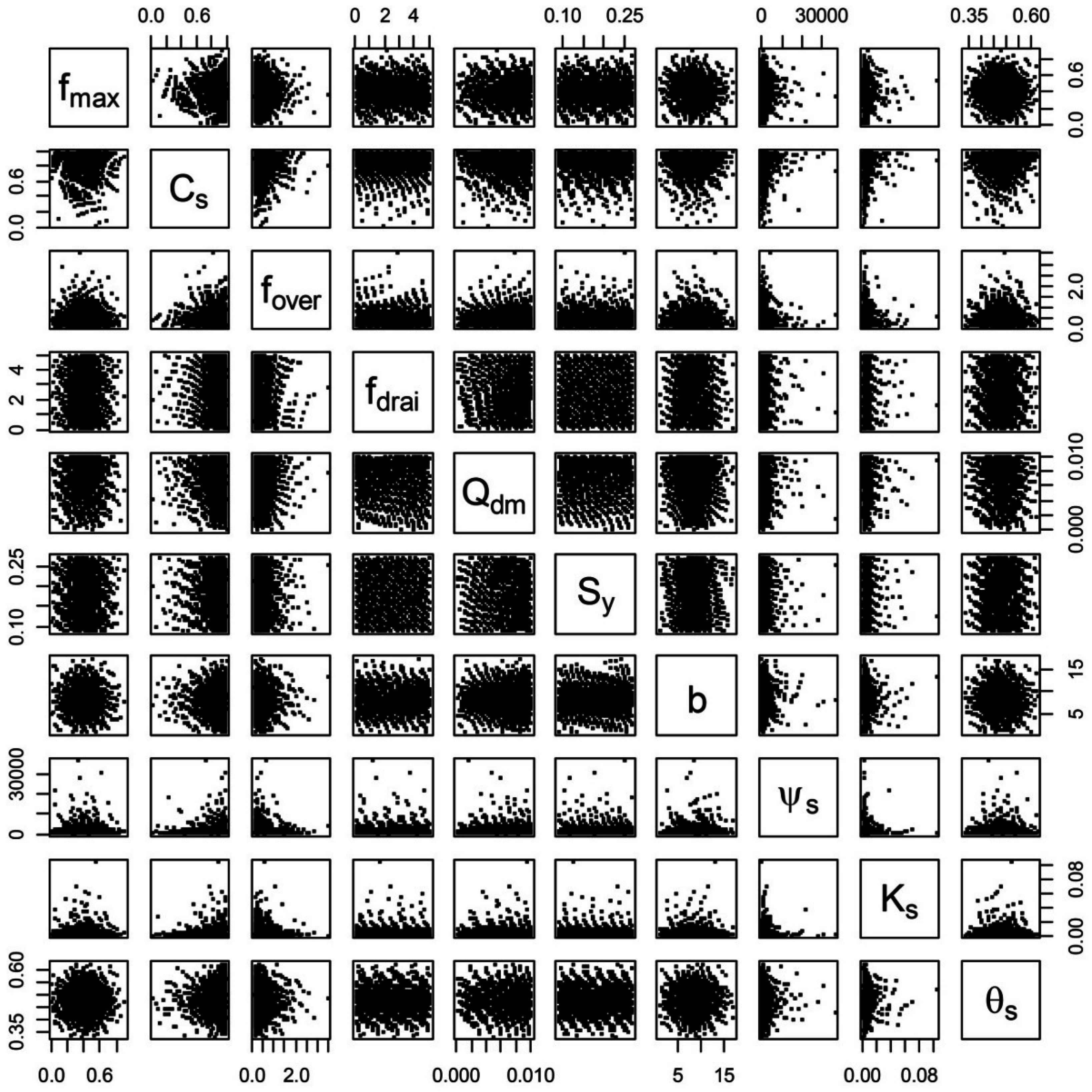
2.2. Model Parameterization

Ten parameters associated with the soil hydrologic process (i.e., surface and subsurface runoff, recharge, soil water transport) are evaluated in this study, and consistent with our earlier studies [4,13]. The parameters are $f_{max}$ (maximum factional saturated area), $C_s$ (shape parameter of topographic index distribution ), $f_{over}$ (decay factor that represents the distribution of surface runoff with depth), $f_{drai}$ (decay factor that represents the distribution of subsurface runoff with depth), $Q_{dm}$ (maximum subsurface drainage), $b$ (Clapp and Hornberger exponent), $S_y$ (specific yield), ${\mathsf{\Psi }}_s$ (saturated soil matrix potential), $K_s$ (hydraulic conductivity), and ${\mathsf{\theta }}_s$ (porosity). Definitions of the 10 selected parameters are in Supplementary Materials Section 1. The uncertainty ranges and prior information about each input parameter are reported in our previous work [13] and are summarized in Supplementary Materials Table S1. Given the prior information, the prior probability density functions (pdfs) of input parameters are derived using the minimum-relative-entropy (MRE) algorithm [42,43]. With the entropy concept, the MRE solution is unique and maximally uncommitted with respect to unknown information given information such as bounds and moments. Therefore, the input parametric uncertainties are fully represented in the form of the MRE prior pdfs, from which samples of the input parameters can be generated using efficient sampling approaches (e.g., quasi Monte Carlo (QMC), Latin Hypercube sampling (LHS)). The details of the MRE algorithm and how to apply it on CLM4 input parameters were introduced in our previous work [4]. Other parameters, like leaf area index and rooting depth of vegetation, may also affect runoff and evapotranspiration. Considering too many parameters at the same time may significantly increase the computational cost and make the SA results unreliable. Therefore, it is preferable to not work directly with a very high-dimensional parameter space, because doing so would make the SA results inconclusive. One solution is to divide all of the CLM4 parameters into several groups for SA study according to their associated physical processes and interactions. We chose the group of parameters associated with the soil hydrologic process in this study. In future work, we will consider adding more parameters or evaluating different groups of parameters.

2.3. Response Variables and Metrics

In this study, we focus on CLM4-simulated runoff and latent heat flux at the MOPEX 0717800 basin from 2000 to 2008. The observed and simulated data to be evaluated include total runoff (runoff), subsurface runoff ($q_{drai}$), surface runoff ($q_{over}$), and latent heat flux (LH). Three metrics are applied to quantitatively evaluate the deviations between the CLM4 simulations and observations: residuals, Nash–Sutcliffe coefficient (NSC) [44,45], and log mean square error (LMSE). Residuals directly measure the deviation between simulation results and observed data, and they favor more of the high flow or high heat flux, because in general the absolute differences between simulations and site observations are bigger when the observations of runoff or latent heat flux are higher. The NSC measures the deviation between simulations and observations during the whole time period of investigation by a nonlinear combination of the correlation, the difference in the mean, and the difference in the variability. It emphasizes high flows or heat flux. LMSE evaluates the difference between simulations and observations during the whole time period of investigation as well. Because the value of runoff usually ranges from 0 to a few hundreds in the units of millimeters per day, the ${\log }_{10}\left(\text{runoff}\right)$ usually ranges from −10 to 2. Therefore, the LMSE puts much more weight on the small runoff values (e.g., near 0 mm/day). The same behavior is true for latent heat flux. Therefore, LMSE places more weight on low flows or low heat flux.

2.4. Effective Sampling and Sensitivity Analysis Methods

2.4.1. Sampling Methods

Input parametric uncertainty can be fully represented in the form of MRE prior pdfs. To reliably evaluate the propagation of such uncertainty using the CLM, samples should be generated from the pdfs to explore all possibilities within the parametric space without introducing undesired bias. However, as the model’s parameter dimensionality increases, the number of samples required for a systematic approach to adequately cover the parametric space becomes unreasonable without efficient sampling methods. Furthermore, the distribution of samples should be consistent with prior information about the parameters.

QMC methods have become increasingly popular over the last two decades because of their faster convergence speeds and effective sampling of high-dimensional parametric space without clumping and gaps [4,46]. In this study, 1024 QMC samples were generated from existing scrambled Sobol sequences [23,47] that ranged from 0 to 1 and were scaled to the actual input parameter ranges listed in our previous work [4]. The QMC samples were projected onto the prior MRE pdfs to construct realizations of the samples in physical space, as shown in Figure 1.

Figure 1. Paired scatterplots of realizations of quasi-Monte Carlo samples for the MOPEX 07147800.

Figure 1. Paired scatterplots of realizations of quasi-Monte Carlo samples for the MOPEX 07147800.

2.4.2. Sensitivity Analysis Approaches

Sensitivity analysis can be based on the direct system model outputs or a surrogate (e.g., a regression model) that can fit the original system outputs to input parameters or factors. Analysis based on the direct outputs avoids the inaccuracy and biases in the regression models, but requires a large amount of sampling points with the necessary number of replicated values of input parameters [48,49], such as those produced using the replicated Latin Hypercube sampling (rLHS) method [50]. For a high-dimensional input parameter space, the number of sampling points is usually more than 10,000 to achieve a converged result [51,52]. This number of sampling points is unaffordable for most studies, particularly when the forward model (e.g., CLM4) is computationally demanding. Therefore, SA based on a regression model is more efficient, especially for high-dimensional input parameter space, because it does not require replicated values of each input parameter. The accuracy of the regression method directly affects the reliability of SA. In this study, four SA approaches are investigated, including analysis of variance (ANOVA) based on the generalized linear model (GLM), generalized cross validation (GCV) based on the multivariate adaptive regression splines (MARS) model, standardized regression coefficients (SRCs) based on the linear regression model (LM), and ANOVA based on support vector machine (SVM). These four approaches are briefly introduced in the following sections.

ANOVA Based on GLM

Assuming the response variable Y (e.g., runoff and/or its metrics) follows a normal distribution, a GLM is fitted with the following starting model:

$$Y_i=c_0+{\displaystyle \sum }_{j=1 to J}^{ }{c}_j{x}_{i,j}+{\mathsf{\epsilon }}_i$$

(1)

where $x_{i,j}$ represents the $i$th realization of the $j$th parameter, which can be original or transformed first-order, two-way interaction, or higher order terms; $c_j$ is the fitted coefficient for the $j$th parameter, which can be calculated by the least squares method [53,54]; $Y_i$ represents the $i$th realization of the response variable, such as $r_{i,t}$, $NS{C}_i$, and $LMS{E}_i$ in this study; and $\mathsf{\epsilon }$ is model-fitting residuals. Generally, use of a GLM is recommended for a monotonic system [33], and it can offer an explicit equation to present the relationship between input and output parameters, which is favorable for engineering applications. ANOVA is a collection of statistical models used to analyze the regression models. In this study, a new regression model built by removing a selected $K$th parameter is

$$Y_i=c_0+{\displaystyle \sum }_{j=1 to J, j\ne K}{c}_j{x}_{i,j}+{\mathsf{\epsilon }}_i$$

(2)

The total deviation difference between the new regression model (Equation (2)) and the completed regression model (Equation (1)) is defined as a quantitative measurement of the importance of parameter $x_K$. This approach summarizes all of the contribution of the parameter $x_K$ in different orders and interaction terms.

GCV Based on the MARS Model

The MARS model is a form of a nonparametric regression technique and can be seen as an extension of linear models that automatically model nonlinearities and interactions between variables. The MARS regression model is of the following form:

$$\widehat{f}\left(x\right)={\displaystyle \sum }_{i=1}^k{c}_i{B}_i\left(x\right)$$

(3)

where $B_i\left(x\right)$ is a basis function, $c_i$ is a coefficient, and $k$ is the number of MARS terms. The basis function $B_i\left(x\right)$ can be a constant, a hinge function [20], or a product of two or more hinge functions, and $x$ represents input parameters. In the MARS model-building process, MARS repeatedly adds paired basis functions to the model, until the residual sum-of-squares (RSS) is smaller than required or the maximum number of terms (specified by the user) is reached. This process is called forward passing and it usually builds an over-fit model, which means the model has a good fit to the training data used to build the model but it will not generalize well to new data. Therefore, the MARS model can be implemented with backward passing to remove terms one by one until the GCV is small enough. GCV is defined as follows:

$$GCV=\frac{RSS}{N{\left(1-\frac{k+P\frac{k-1}{2}}{N}\right)}^2}$$

(4)

where $N$ is the number of observed system outputs, and $P$ is a penalty coefficient, which is about 2 or 3 [20]. With MARS terms dropped, the RSS always increases, but the denominator of Equation (4) increases as well, so the GCV is a form of regularization that trades off goodness-of-fit against model complexity. After the MARS model is specified, the GCV can be used to quantitatively measure the importance of input parameters. For a developed MARS model, when all of the terms related to an input parameter are removed, the RSS and the number of MARS terms ($k$) will change, which leads to GCV changes. Conversely, the GCV change due to removal of the MARS model terms related to a parameter can be used as a quantitative measure of how much the regression model depends on the removed input parameter, that is, the importance of the corresponding input parameter. The MARS model theoretically can offer better interpolation than the GLM for a nonmonotonic nonlinear system, so the measurement of input parameter importance is supposed to be more reliable. In addition, the convergence behavior and performance with the number of sampling points for the MARS model and GLM are different, as demonstrated and discussed in Section 3.3.

SRC Based on the LM

A linear polynomial regression analysis assumes the following form:

$$Y_m={\displaystyle \sum }_{k=1}^n{b}_k{x}_k^m+b_0+{\mathsf{ϵ}}_m$$

(5)

For the $m$-th sample points, $x$ are the input parameters, $b$ are the coefficients to be determined, $Y$ is the output from the computational model, and $\mathsf{ϵ}$ is the discrepancy between the simulation model output and the regression results. For the $k$-th input parameter, the SRC is defined as [21,55]

$$SRC=\frac{b_k{\widehat{s}}_k}{\widehat{s}}$$

(6)

where

$$\widehat{s}={\left[\frac{1}{M-1}{\displaystyle \sum }_{m=1}^M{\left(Y_m-\overline{Y}\right)}^2\right]}^{1/2}\text{ and }{\widehat{s}}_k={\left[\frac{1}{M-1}{\displaystyle \sum }_{m=1}^M{\left(x_k^m-{\overline{x}}_k\right)}^2\right]}^{1/2}$$

(7)

and $M$ is the total number of sampling sets, and symbol $\overline{( )}$ stands for the mean value.

ANOVA Based on SVM

The basic idea of the SVM regression model is to find a function that deviates most from the actually obtained outputs for all of the training data and, at the same time, is as flat as possible [31,32]. For a linear function in the form of

$$Y_i={\displaystyle \sum }_{j=1 to J}^{ }{a}_j{x}_{i,j}+b_i$$

(8)

where $a_j$ is the weighting coefficient, $b_j$ is a translation coefficient, and $x_{i,j}$ is $j_{th}$ input parameter for the $i_{th}$ sample, the formulated SVM approximation is

$$\text{minimizing }\frac{1}{2}{\left|a\right|}^2$$

(9)

$$\text{subject to }\{\begin{array}{c}{Y}_i-{\displaystyle \sum }_{j=1 to J}^{ }{a}_j{x}_{i,j}+b_i\le \mathsf{ϵ}\\ {\displaystyle \sum }_{j=1 to J}^{ }{a}_j{x}_{i,j}+b_i-Y_i\le \mathsf{ϵ}\end{array}$$

where $\mathsf{ϵ}$ is the most required deviation. Because the SVM assumption may be unrealistic in general, a slack variable is used to control the tradeoff between flatness and how much deviation is tolerated. Coefficients $a_j$ can be calculated from the optimization problem (Equation (9)), and the $b_i$ can be calculated using Karush-Kuhn-Tucker (KKT) conditions [33]. More details regarding SVM can be found in references [31,32,33]. The ANOVA for SVM is designed to be the total deviation difference between a new regression model (Equations (10) and(11)) that is kicked out a selected input parameter ($x_K$) and the completed regression model (Equations (8) and (9)) is defined as a quantitative measurement of the importance of parameter $x_K$.

$$Y_i={\displaystyle \sum }_{j=1 to J, j\ne K}^{ }{a}_j{x}_{i,j}+b_i$$

(10)

$$\text{minimizing }\frac{1}{2}{\left|a\right|}^2$$

(11)

$$\text{subject to }\{\begin{array}{c}{Y}_i-{\displaystyle \sum }_{j=1 to J, j\ne K}^{ }{a}_j{x}_{i,j}+b_i\le \mathsf{ϵ}\\ {\displaystyle \sum }_{j=1 to J, j\ne K}^{ }{a}_j{x}_{i,j}+b_i-Y_i\le \mathsf{ϵ}\end{array}$$

3. Results and Discussion

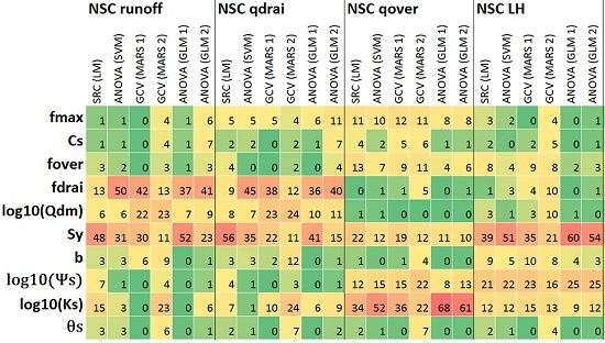
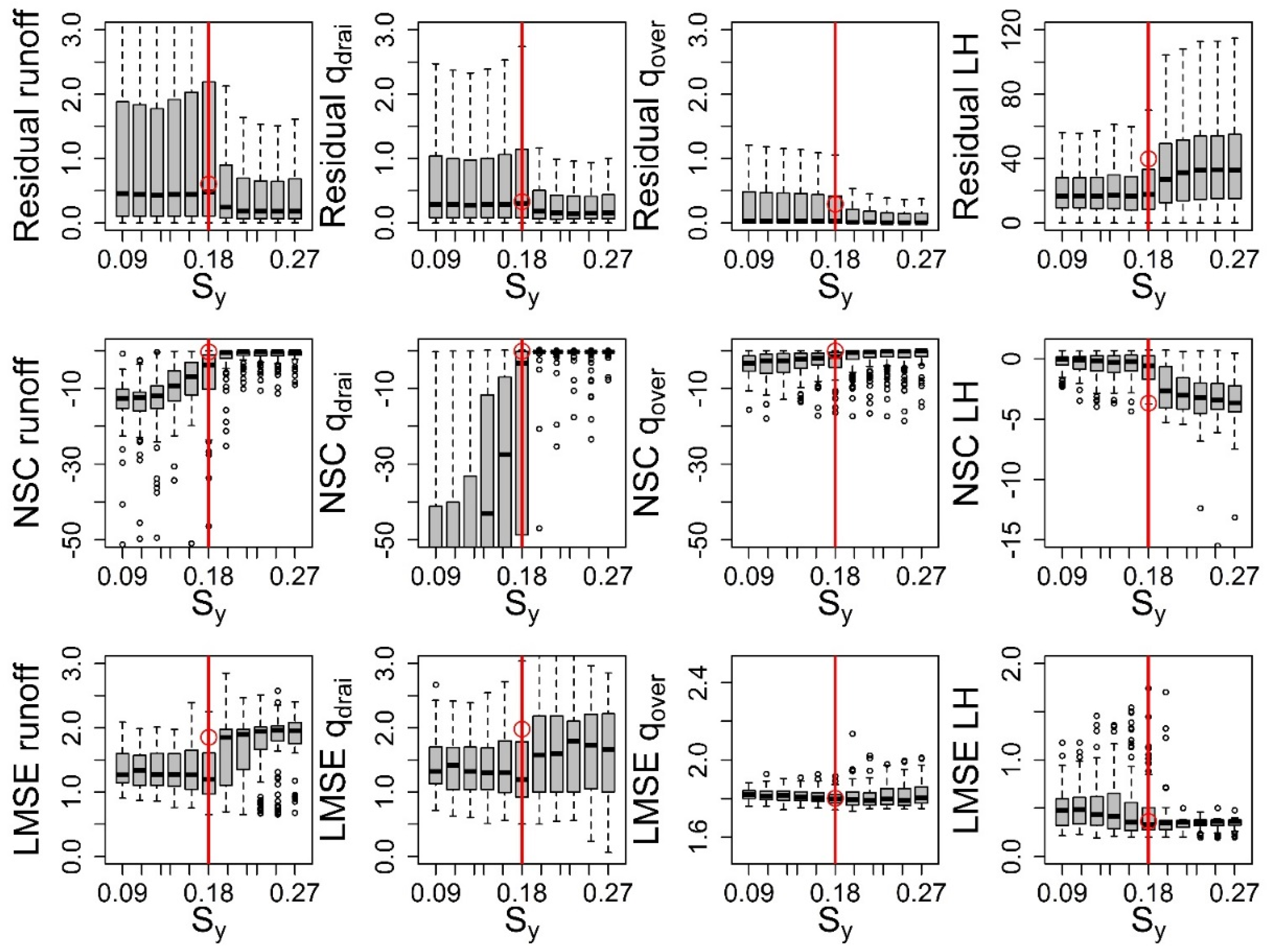
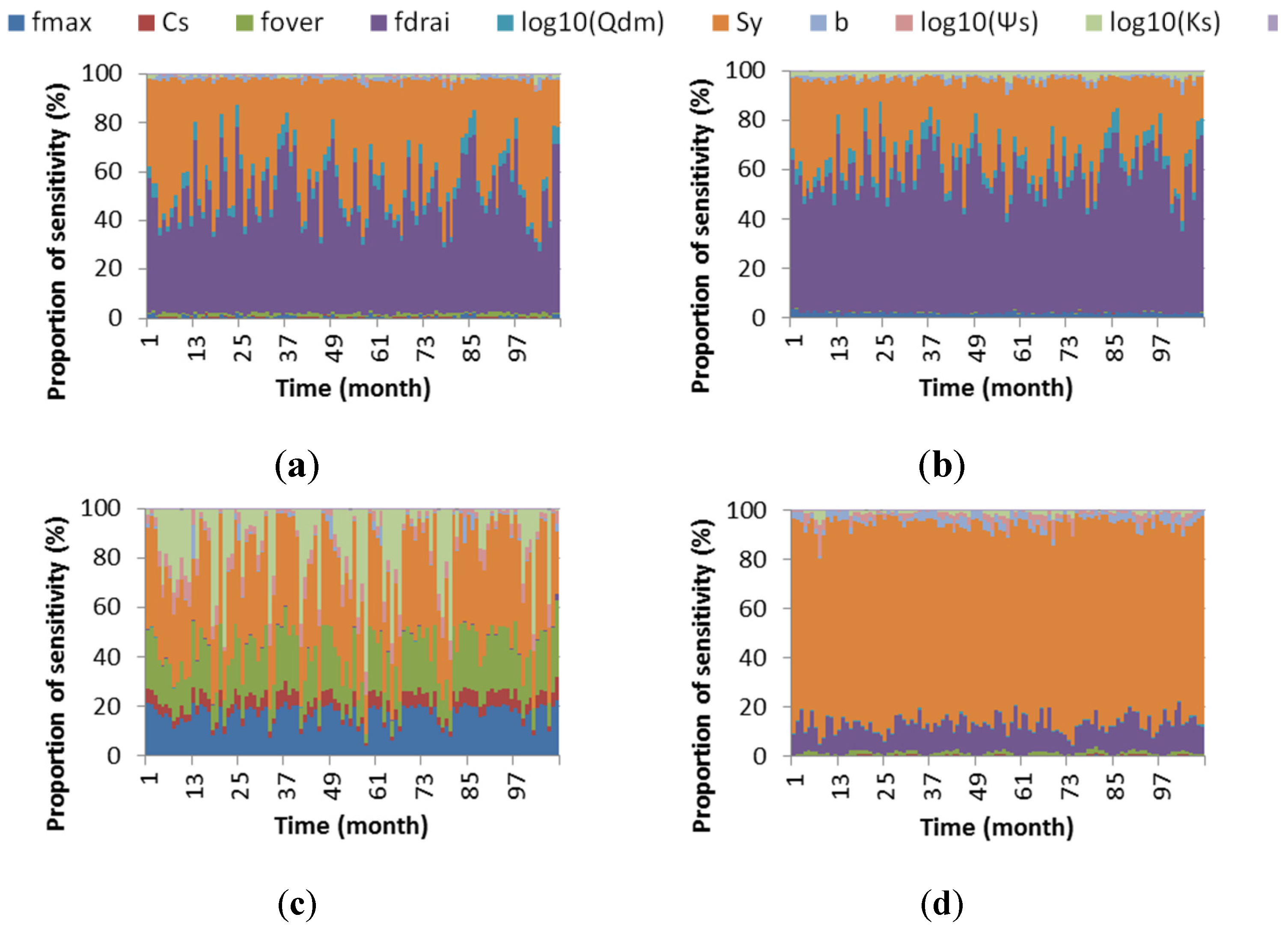
3.1. Effects of Choices of Response Variables/Metrics

Figure 2 shows boxplots [56,57,58] that compare the residuals for different response variables and metrics as a function of input parameters $S_y$. In this study, $S_y$ is one of the input parameters that show significant sensitivity relative to the deviation between the simulation and observation data, so we only show the boxplots of $S_y$ to be concise. The boxplots for other input parameters are shown in Figures S1–S3 in the Supplementary Materials Section 3. As mentioned in Section 2.1, a 3.8 m soil column is used to simulate the soil moisture redistribution; it is discretized into 10 layers and an unconfined aquifer with a prescribed storage capacity and specific yield ($S_y$) is added to the bottom of the soil column that could potentially be recharged or supply water to the soil column. Generally, a large value of $S_y$ leads to more water exchange between soil layers and the aquifer. At this site, such exchange seems to reduce overland flow ($q_{over}$) and consequently increases subsurface runoff ($q_{drai}$) by infiltrating more water into the subsurface. The recharge of the aquifer enhances percolation of water from shallow to deep soil layers, reduces available water to the shallow rooted vegetation dominated by cropland and grassland, and therefore the latent heat flux (LH). On the other hand, under extremely wet conditions, both $q_{drai}$ and LH are high because there is sufficient soil water supply to both. Therefore, there is no simple linear relationship between $S_y$ and LH. The total amount of LH may be affected nonlinearly by the combination of $S_y$and other parameters. In Figure 2, the vertical red line is the default value of $S_y$, which is 0.18 at this site. The red circles are the corresponding metric value obtained by using the default values for all of the selected 10 input parameters. The boxplots of residual and NSC of total runoff, subsurface runoff $q_{drai}$, and surface runoff $q_{over}$ indicate that increased values of $S_y$ can reduce the deviations between simulation and observation data. The boxplots of LMSE of total runoff, $q_{drai}$, and $q_{over}$ do not indicate an obvious preference of $S_y$ value that can reduce the deviations. For latent heat (LH), residual and NSC indicate that decreased values of $S_y$ can reduce the deviations, while LMSE indicates that increased values of $S_y$ can reduce the deviations. In summary, the boxplots of various metrics of streamflow indicate that a large value of $S_y$ can significantly reduce the model deviations. The metrics of LH indicate that simultaneous adjustments of $S_y$ and other parameters are required to further reduce the deviation for LH. Many trials in the boxplots show that NSC LH approaches 1 and LMSE LH approaches 0 simultaneously with large $S_y$ values. It should be noted that the boxplot is mainly used for qualitatively showing the significance of the metrics variation due to changes in the input parameters and the potential for reducing the deviations by adjusting parameter values. It is impossible to find the optimal input parameter value directly from the boxplot. Systematic calibration of input parameters will be discussed in our future work.

Figure 2. Boxplots for different response variables and metrics as a function of input parameters specific yield ($S_y$).

Figure 2. Boxplots for different response variables and metrics as a function of input parameters specific yield ($S_y$).

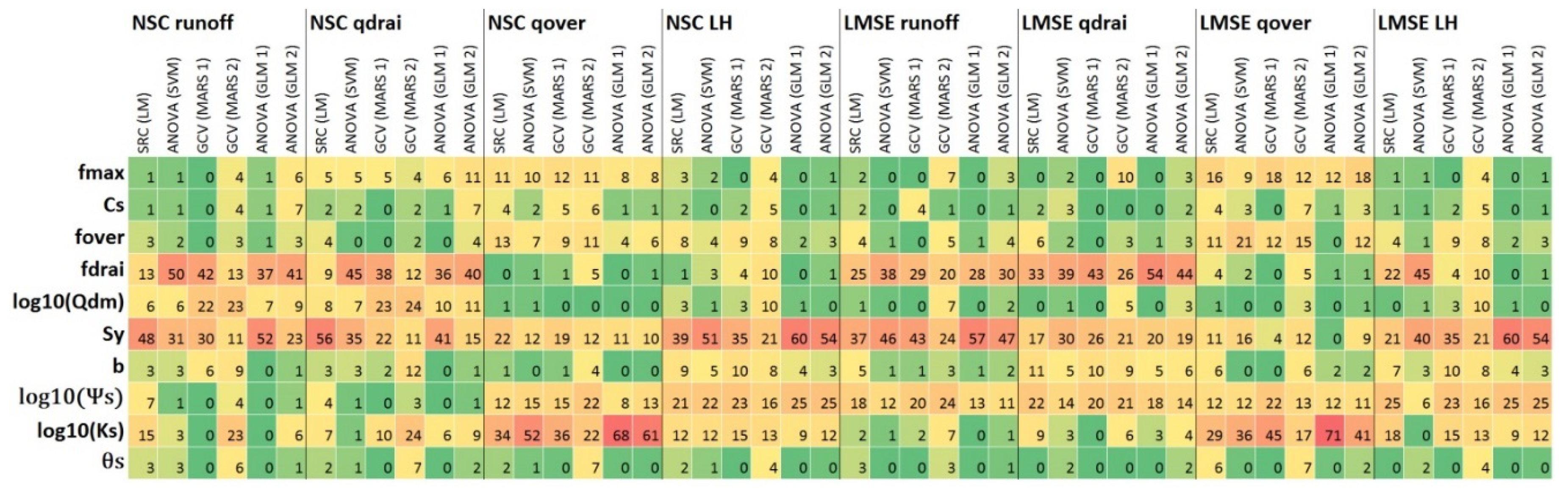
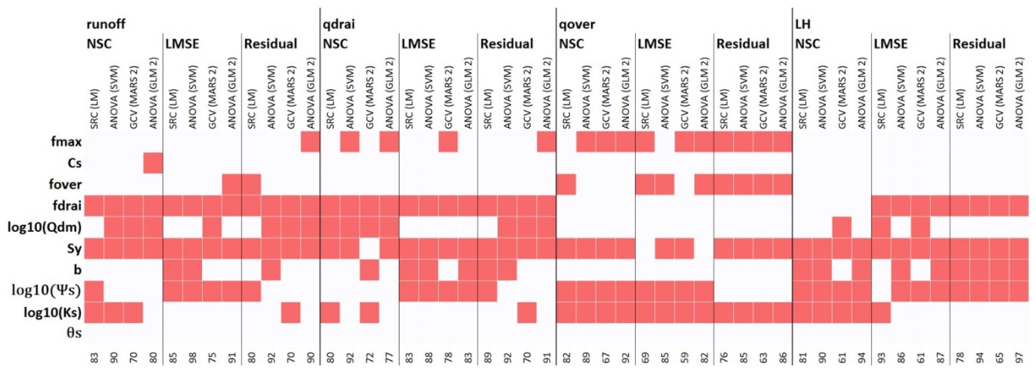
3.2. Effects of Choices of SA Approach

The preceding analyses provide qualitative information (Figure 2 and Figures S1–S3) about which parameters are more significant, and therefore need to be adjusted when calibrating the CLM4, and they indicate the direction of such adjustments. Sensitivity analysis approaches can quantitatively measure the importance of each input parameter, but different approaches usually yield different evaluations, especially for complicated systems. In many cases, it is hard to justify which approach is best for the particular system. For example, ANOVA based on a GLM usually enlarges the importance of top-ranked parameters, so it is efficient for parameter screening and reduced-order model development. GCV based on a MARS model usually more evenly distributes the contribution of variance among all of the parameters, so it may enlarge the importance of lower ranked parameters. There is no universal method that can accurately evaluate the importance of input parameters for every system, but GCV is considered a more reliable SA approach for nonmonotonic nonlinear systems. It is reasonable to compare the measurements/findings from multiple approaches, such as ANOVA, GCV, and SRC, or combine them with qualitative analysis to provide supplementary information to each other and to remove ambiguities from the conclusions. As mentioned above, the reliability of the regression model affects the accuracy of the sensitivity measurement. Generally, a higher order regression model can fit the training set better, which means that an SA based on higher order regression model is more accurate. However, a high-order regression model may over-fit the training set, e.g., fitting the noises or outliers in the system, which may reduce the reliability of the SA results. Therefore, an appropriate order of the regression model is critical for SA. In this study, a first-order GLM, MARS, LM, and SVM model can provide a correlation coefficient ($R^2$) of about 0.2 to 0.4, and a second-order GLM or MARS model can fit the system $R^2$ of around 0.8 to 0.9. A third-order GLM or MARS model can provide a $R^2$ reaching 0.99, but the resulting relationships are hard to interpret physically, and likely to be over-fitted statistically given the high number of coefficients to be fitted with limited sample sets; therefore, third or higher order models are not considered in this study.

Figure 3 shows the sensitivity score of the input parameters for the NSC and LMSE of runoff, $q_{drai}$, $q_{over}$, and LH derived using six different approaches. They are SRC based on LM, ANOVA based on SVM, GCV based on first- and second-order MARS, and ANOVA based on first- and second-order GLM. The score stands for the percentage of the contributions to the total variance of the investigated output response from each input parameter’s uncertainty. The warm color (red) stands for more important, and the cold color (green) means less important. Generally, $S_y$ shows considerable importance for most response variables and metrics. $f_{drai}$ is important for total runoff, subsurface runoff, and LH, while $lo{g}_{10}(K_s)$ is more important for surface runoff and LH. $lo{g}_{10}({\mathsf{\Psi }}_s)$ is relatively important for surface runoff and latent heat as well. ${\log }_{10}(Q_{dm})$ also shows considerable impact on $q_{drai}$ and LH. In general, the six approaches show consistent results.

Figure 3. Sensitivity scores for different response variables/metrics and SA approaches.

Figure 3. Sensitivity scores for different response variables/metrics and SA approaches.

Figure 4 shows the proportion of sensitivity of ANOVA based on the first-order GLM for residuals of runoff, $q_{drai}$, $q_{over}$, and LH in 108 months to investigate the seasonal patterns of parameter importance. The proportion of sensitivity is calculated for each month separately. For the residuals of total runoff (Figure 4a), $S_y$ and $f_{drai}$ are dominant in the contributions to the residuals between simulations and observed data in all of the 108 months. $f_{drai}$ is more important in winter and $S_y$ is more important in summer. Using the residual of $q_{drai}$ as the response variable (Figure 4b), the sensitivity scores are almost the same as using total runoff. Regarding the residual of $q_{over}$ (Figure 4c), $f_{max}$, $f_{over}$, $S_y$, and $lo{g}_{10}(K_s)$ are the top four input parameters in most of the 108 months$f_{max}$, $f_{over}$, and $S_y$ are more important in winter and less important in summer, while $lo{g}_{10}(K_s)$ is more important in summer and less important in winter. Figure 4d shows the residuals of LH. $S_y$, as the critical parameter, is more important in winter and less important in summer. For the investigated site, $S_y$ mainly controls (indirectly) how fast the water can percolate through the soil layers; it modifies the lower boundary condition of the 1-D Richards equation by recharging the underlying aquifer layer during and after precipitation. Fast percolation leads to less overland flow and shallow-layer soil moisture, and therefore less LH. It should be noted that the proportion of sensitivity shown here is only for ANOVA based on the first-order GLM. The figures showing the proportion of sensitivity variation with time for other SA approaches are in Supplementary Materials Figure S4, which assigns a relatively lower proportion of sensitivity to $S_y$.

Figure 5 summarizes the four most important input parameters (red blocks) for different response variables (total runoff, $q_{drai}$,$q_{over}$, and LH), metrics (NSC, LMSE, and residual), and four SA approaches (SRC based on LM, ANOVA based on SVM, GCV based on second-order MARS, and ANOVA based on second-order GLM). The total contributions percentages of the top four input parameters are also listed in the bottom line in Figure 5. ANOVA based on GLM or SVM indicates that the top four important parameters are adequate to calibrate the CLM4, because they account for 80% to 90% of the variations in response variables. However, GCV and SRC show that the top four most important parameters only contribute 60% to 80% to the total variability of the response variables. The quantitative importance measurement provides a guideline for further model calibration for CLM4. For example, using the four most important parameters listed in Figure 5 as unknowns, one can efficiently calibrate CLM by adjusting the parameters to match the total runoff simulations; adding the fifth and sixth important parameters (i.e., $b$ and ${\mathsf{\theta }}_s$) would have little impact on matching runoff observations and CLM4 predictions.

Figure 4. Proportion of sensitivity for residual in 108 months. (a) Residual of total runoff (runoff) ANOVA (GLM 1st order); (b) Residual of subsurface runoff (qdrai) ANOVA (GLM 1st order); (c) Residual of surface runoff (qover) ANOVA (GLM 1st order); (d) Residual of latent heat (LH) ANOVA (GLM 1st order).

Figure 4. Proportion of sensitivity for residual in 108 months. (a) Residual of total runoff (runoff) ANOVA (GLM 1st order); (b) Residual of subsurface runoff (qdrai) ANOVA (GLM 1st order); (c) Residual of surface runoff (qover) ANOVA (GLM 1st order); (d) Residual of latent heat (LH) ANOVA (GLM 1st order).

Figure 5. The four most important input parameters (red blocks) for different response variables (total runoff, $q_{drai}$, $q_{over}$, and LH), metrics (NSC, LMSE, and residual), and four SA approaches (SRC based on LM, ANOVA based on SVM, GCV based on second-order MARS, and ANOVA based on second-order GLM).

Figure 5. The four most important input parameters (red blocks) for different response variables (total runoff, $q_{drai}$, $q_{over}$, and LH), metrics (NSC, LMSE, and residual), and four SA approaches (SRC based on LM, ANOVA based on SVM, GCV based on second-order MARS, and ANOVA based on second-order GLM).

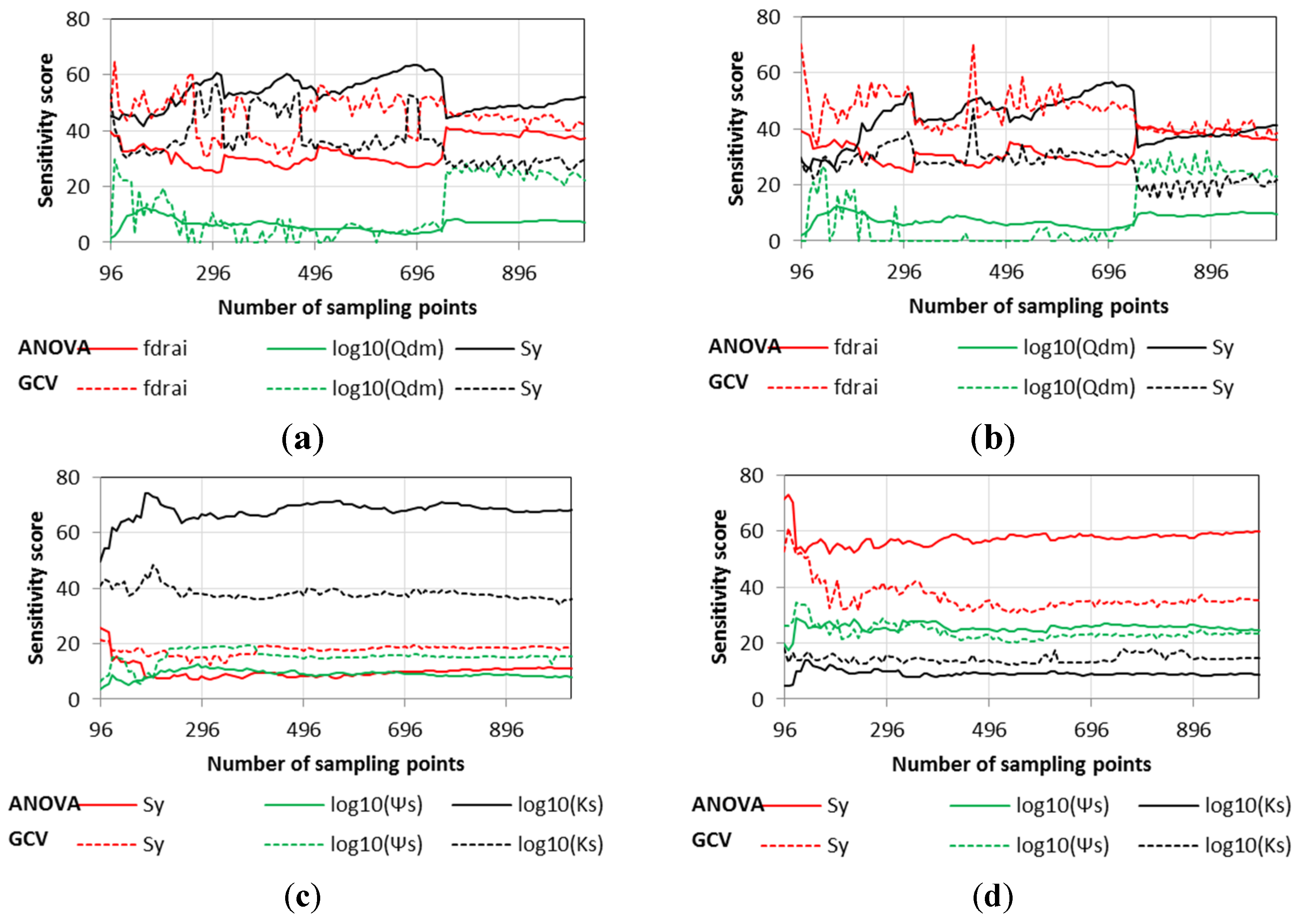
3.3. Convergence, Under-Sampling Issues, and Model Verification

As mentioned in Section 3.2, different SA approaches may lead to different important measurement results for input parameters. Moreover, the convergence speed of the SA approach may vary, and the SA approach with higher convergence speed is always preferred. The convergence speed also varies with different response variables. Figure 6 shows the comparison of the convergence of sensitivity scores for different response variables (NSC of total runoff, $q_{drai}$, $q_{over}$, and LH) and SA approaches (ANOVA based on first-order GLM and GCV based on first-order MARS). The convergence curves for LMSE and second-order regression models are shown in Figure S5 in the Supplementary Materials, where only the three most important input parameters are compared. For the NSCs of total runoff and $q_{drai}$ (Figure 6a,b), around 700 sampling points are needed to get a converged sensitivity measurement, and the GCV measurement still shows small fluctuations after 700 sampling points. ANOVA measurement seems to be a little more stable than GCV. For the NSC of $q_{over}$ (Figure 6c), around 250 sampling points are needed for stabilized sensitivity scores; similarly, GCV shows slightly larger fluctuations than ANOVA. For the NSC of LH (Figure 6d), 250 samples are needed, while the LMSE of LH needs about 400 sampling points. In summary, GCV and ANOVA can both achieve relatively stable measurements using a reasonable number of sampling points. The sensitivity score results converge slightly slower than the ANOVA results. From this point of view, the ANOVA results are more reliable with limited samples. In addition, the convergence curves provide guidance on the reliability of SA with different numbers of sampling points. For the field site of investigation, the recommended number of sampling points would be at least 400 in order to fully understand and therefore use the calibratable portion of the total variability in the observations. If the research focus is to separate the dominant and secondary input parameters, 250 or even 128 sampling points can provide relatively reliable results in ranking the parameter significance.

Figure 6. Sensitivity scores convergence for different response variables and SA approaches. (a) NSC of runoff (1st order); (b) NSC of qdrai (1st order); (c) NSC of qover (1st order); (d) NSC of LH (1st order).

Figure 6. Sensitivity scores convergence for different response variables and SA approaches. (a) NSC of runoff (1st order); (b) NSC of qdrai (1st order); (c) NSC of qover (1st order); (d) NSC of LH (1st order).

4. Conclusions

In this study, different SA approaches were applied to various combinations of input parameters and CLM4 output metrics in order to evaluate the consistency and robustness of the conclusions about parameter sensitivity and the possibility of model optimization. Generally, $S_y$ shows significant impacts on the deviation between the CLM4 simulations and observed conditions of the investigated MOPEX 07147800 basin. $f_{drai}$ is important for $q_{drai}$ and LH, while $lo{g}_{10}\left(K_s\right)$ and $lo{g}_{10}({\mathsf{\Psi }}_s)$ are important for $q_{over}$ and LH. ${\log }_{10}(Q_{dm})$ also shows considerable impact on $q_{drai}$ and LH. The soil hydraulic parameters, $K_s$ and ${\mathsf{\Psi }}_s$, ${\mathsf{\theta }}_s$, and $b$, affect the maximum infiltration capacity and therefore have significant impact on $q_{over}$. According to the default global data set for CLM4, the prior ranges of ${\mathsf{\theta }}_s$ and $b$ are much smaller than those of $K_s$ and ${\mathsf{\Psi }}_s$, so their impacts on the variation of surface runoff $q_{over}$ seem to be smaller. $f_{max}$ and $f_{over}$ are also critical parameters controlling $q_{over}$, and because they are closely related to topography and were estimated from high-resolution digital elevation models, their default values and ranges were relatively accurate with small uncertainties and impacts on model outputs. The subsurface runoff, $q_{drai}$, is exponentially dependent on $f_{drai}$ and $S_y$, and linearly dependent on $Q_{dm}$. Furthermore, the hydrologic parameters investigated in this study would influence not only runoff, but also soil moisture, which is key to the simulations of latent heat flux. Therefore, the parameters important for runoff are usually important for latent heat flux as well.

All of the investigated SA approaches yield consistent findings and show that in general at least three among the top four parameters are confirmed by two or more SA approaches, although the quantitative measures of parameter importance vary among the SA approaches. ANOVA indicates that the four most important parameters contribute around 80% to 90% of the variations in response variables, which means that these four parameters are adequate to calibrate CLM4. GCV and SRC indicate that the four most important parameters only contribute around 60% to 80% of the variations in response variables, and the calibration might need the fifth and even sixth most important parameters to help reduce the mismatches between runoff observations and CLM simulations. Theoretically, the MARS model can be used to build a regression model that perfectly matches the training set (here the CLM4 simulations), because the MARS model can keep adding hinge functions into the model to reduce the deviations to 0. Therefore, the MARS model provides a more accurate regressed model than the other three regression models. However, a more accurate regression model does not guarantee that the corresponding sensitivity measurement will be more reliable, because the training data not only provide information about the relationship between input and output parameters, but also contain noises associated with errors and uncertainties in observation-based data and numerical errors in CLM4 simulations. The regression model that perfectly matches the training data set might be over-fitted; therefore, it is reasonable to use multiple models to provide complementary information. Considering that the four SA approaches provide similar sensitivity measurements for most response variables in this study, we believe they are reliable for the study site.

The first- and second-order regression models were used to fit the response variables, and the impacts of the order of regression models on the sensitivity measurement were investigated. If the relationships between response variables and input parameters are linear, the order of regression models do not affect the sensitivity measurement much, e.g., the NSC of $q_{over}$, NSC of LH, and LMSE of $q_{drai}$. If the relationships between response variables and input parameters are mostly quadratic, the order of regression models affect the sensitivity measurement, e.g., the NSC of runoff, NSC of $q_{drai}$, LMSE of runoff, and LMSE of $q_{over}$.

This study also evaluated the effectiveness of quantitative SA approaches on different types of CLM4 output data, including runoff and latent heat fluxes. Different metrics of these simulated deviations are treated as response variables in the SA, which identifies the parameters dominating the deviations and therefore should be included in the model calibration or parameter inversion design. Depending on the purpose of matching the whole time series (low, high, and medium values) or just the extreme events (e.g., high runoff/LH), different sets of parameters should be inverted. For example, in model calibration on subsurface runoff, if the purpose is matching whole time series, $S_y$, $f_{drai}$, and ${\log }_{10}(Q_{dm})$ would be the parameters to be adjusted, and adjustment of $f_{max}$ and $lo{g}_{10}\left(K_s\right)$ might also be considered if higher accuracy numerical prediction is expected. If the calibration focuses on a low flow regime, $S_y$, $f_{drai}$, $lo{g}_{10}({\mathsf{\Psi }}_s)$, ${\log }_{10}(Q_{dm})$, and $f_{over}$ should be included as unknowns. In addition, adopting different SA approaches may yield different ideas of inversion setup, and such differences are more obvious for parameters whose contributions are somewhere between dominant and secondary. The common parameters identified to be important by different SA approaches are of high priority to be optimized for reducing the discrepancies between runoff/LH observations and model simulations. It is reasonable to conduct joint inversion of multiple data or metrics to provide supplementary information to each other.

As mentioned in Section 2, the subsurface and surface runoffs are derived from total runoff. Because the subsurface runoff dominates the total runoff in the studied basin, the SA results are almost the same for total runoff and subsurface runoff. The metrics of NSC and LMSE indicate that the separation of subsurface runoff from total runoff helps improve the matches between simulated $q_{drai}$ and observations. Because the temporal variations in total runoff and surface runoff ($q_{over}$) are mainly caused by precipitation, the effects of the input parameters may be concealed by the temporal variations in precipitation, especially the short-term components. Separating the subsurface flow ($q_{drai}$) from total runoff might weaken the influence of precipitation variations and enhance the contributions from the input parameters. As a result, adjustments of the input parameters can clearly modify the simulated $q_{drai}$, and therefore it could be more favorable to use $q_{drai}$ for model calibration.

The convergence behaviors (as a function of the number of samples) of the SA approaches provide guidance for the number of sampling points to be used for reliable SA and parameter identifiability study. For the study site, the recommended number of sample sets is at least 400. If the focus is to separate the dominant and secondary input parameters, 250 or even 128 sampling points are acceptable [4].

References

1. Henderson-Sellers, A.; Pitman, A.J.; Love, P.K.; Irannejad, P.; Chen, T.H. The Project for Intercomparison of Land-Surface Parameterization Schemes (Pilps)—Phase-2 and Phase-3. Bull. Am. Meteorol. Soc. 1995, 76, 489–503. [Google Scholar] [CrossRef]
2. Henderson-Sellers, A.; Chen, T.H.; Nakken, M. Predicting global change at the land-surface: The project for intercomparison of land-surface parameterization schemes (PILPS) (phase 4). In Proceedings of the Seventh American Meteorological Society (AMS) symposium on global change studies, Atlanta, GA, USA, 28 January–2 February 1996; pp. 59–66.
3. Bastidas, L.A.; Hogue, T.S.; Sorooshian, S.; Gupta, H.V.; Shuttleworth, W.J. Parameter sensitivity analysis for different complexity land surface models using multicriteria methods. J. Geophys. Res. 2006, 111. [Google Scholar] [CrossRef]
4. Hou, Z.; Huang, M.; Leung, L.R.; Lin, G.; Ricciuto, D.M. Sensitivity of surface flux simulations to hydrologic parameters based on an uncertainty quantification framework applied to the Community Land Model. J. Geophys. Res. 2012, 117. [Google Scholar] [CrossRef]
5. Göhler, M.; Mai, J.; Cuntz, M. Use of eigendecomposition in a parameter sensitivity analysis of the Community Land Model. J. Geophys. Res. Biogeosci. 2013, 118, 904–921. [Google Scholar] [CrossRef]
6. Nasybulin, E.; Xu, W.; Engelhard, M.H.; Nie, Z.; Burton, S.D.; Cosimbescu, L.; Gross, M.E.; Zhang, J.-G. Effects of Electrolyte Salts on the Performance of Li-O-2 Batteries. J. Phys. Chem. C 2013, 117, 2635–2645. [Google Scholar] [CrossRef]
7. Oleson, K.W.; Dai, Y.J.; Bonan, G.B.; Bosilovich, M.; Dickinson, R.; Dirmeyer, P.; Hoffman, F.M.; Houser, P.R.; Levis, S.; Niu, Y.; et al. Technical Description f Version 4.0 of the Community Land Model (CLM); National Center for Atomospheric Research: Boulder, CO, USA, 2010. [Google Scholar]
8. Lawrence, D.M.; Oleson, K.W.; Flanner, M.G.; Thornton, P.E.; Swenson, S.C.; Lawrence, P.J.; Zeng, Z.; Yang, Z.L.; Levis, S.; Sakaguchi, K.; et al. Parameterization Improvements and Functional and Structural Advances in Version 4 of the Community Land Model. J. Adv. Model. Earth Syst. 2011, 3, 27. [Google Scholar]
9. Leng, G.; Huang, M.; Tang, Q.; Gao, H.; Leung, L.R. Modeling the effects of groundwater-fed irrigation on terrestrial hydrology over the conterminous United States. J. Hydrometeorol. 2014, 15, 957–972. [Google Scholar] [CrossRef]
10. Lei, H.; Huang, M.; Leung, R.; Yang, D.; Shi, X.; Mao, J.; Hayes, D.J.; Schwalm, C.R.; Wei, Y.; Liu, S. Sensitivity of global terrestrial gross primary production to hydrologic states simulated by the Community Land Model using two runoff parameterizations. J. Adv. Model. Earth Syst. 2014, 6. [Google Scholar] [CrossRef]
11. Stöckli, R.; Lawrence, D.M.; Niu, G.-Y.; Oleson, K.W.; Thornton, P.E.; Yang, Z.-L.; Bonan, G.B.; Denning, A.S.; Running, S.W. Use of FLUXNET in the Community Land Model development. J. Geophys. Res. 2008, 113. [Google Scholar] [CrossRef]
12. Niu, G.-Y.; Yang, Z.-L.; Dickinson, R.; Dickinson, R.; Gulden, L.E.; Gulden, L.E. A simple TOPMODEL-based runoff parameterization (SIMTOP) for use in global climate models. J. Geophys. Res. 2005, 110. [Google Scholar] [CrossRef]
13. Huang, M.; Hou, Z.; Leung, L.R.; Ke, Y.; Liu, Y.; Fang, Z.; Sun, Y. Uncertainty Analysis of Runoff Simulations and Parameter Detectability in the Community Land Model—Evidence from MOPEX Basins and Flux Tower Sites. J. Hydrometeorol. 2013, 14, 1754–1772. [Google Scholar] [CrossRef]
14. Liu, Y.; Gupta, H.V.; Sorooshian, S.; Bastidas, L.A.; Shuttleworth, W.J. Exploring parameter sensitivities of the land surface using a locally coupled land-atmosphere model. J. Geophys. Res. Atmos. 2004, 109. [Google Scholar] [CrossRef]
15. Van Griensven, A.; Meixnera, T.; Grunwaldb, S.; Bishopb, T.; Diluzioc, M.; Srinivasand, R. A global sensitivity analysis tool for the parameters of multi-variable catchment models. J. Hydrol. 2006, 324, 10–23. [Google Scholar] [CrossRef]
16. Campolongo, F.; Cariboni, J.; Saltelli, A. An effective screening design for sensitivity analysis of large models. Environ. Model. Softw. 2007, 22, 1509–1518. [Google Scholar] [CrossRef]
17. Borgonovo, E.; Castaings, W.; Tarantola, S. Model emulation and moment-independent sensitivity analysis: An application to environmental modelling. Environ. Model. Softw. 2012, 34, 105–115. [Google Scholar] [CrossRef]
18. Pan, W.; Bao, J.; Lo, C.; Lai, K.; Agarwal, K.; Koeppel, B.J.; Khaleel, M. A general approach to develop reduced order models for simulation of solid oxide fuel cell stacks. J. Power Sources 2013, 232, 139–151. [Google Scholar] [CrossRef]
19. Bao, J.; Xu, Z.; Lin, G.; Fang, Y. Uncertainty quantification for evaluating impacts of caprock and reservoir properties on pressure buildup and ground surface displacement during geological CO2 sequestration. Greenh. Gases Sci. Technol. 2013, 3, 338–358. [Google Scholar] [CrossRef]
20. Friedman, J.H. Multivariate Adaptive Regression Splines. Ann. Stat. 1991, 19, 1–67. [Google Scholar] [CrossRef]
21. Aiken, L.S.; West, S.G. Multiple Regression: Testing and Interpreting Interactions; Sage Publications Inc.: Thousand Oaks, CA, USA, 1991. [Google Scholar]
22. Morris, M.D. Factorial sampling plans for preliminary computational experiments. Technometrics 1991, 33, 161–174. [Google Scholar] [CrossRef]
23. Sobol, I.M. On the distribution of points in a cube and the approximate evaluation of integrals. USSR Comput. Math. Math. Phys. Engl. Transl. 1967, 7, 86–112. [Google Scholar] [CrossRef]
24. Friedman, J.H. Fitting funcctions to noisy data in high dimensions. In Proceedings of the 20th Symposium on the Interface, Reston, VA, USA, 20–23 April 1988.
25. Anscombe, F.J. The Validity of Comparative Experiments. J. R. Stat. Soc. Ser. A 1948, 111, 181–211. [Google Scholar] [CrossRef]
26. Box, G.E.P. Some Theorems on Quadratic Forms Applied in the Study of Analysis of Variance Problems, I. Effect of Inequality of Variance in the One-Way Classification. Ann. Math. Stat. 1954, 25, 290–302. [Google Scholar] [CrossRef]
27. McCullagh, P.; Nelder, J. Generalized Linear Models, 2nd ed.; CRC press: Boca Raton, FL, USA, 1989. [Google Scholar]
28. Chambers, J.M.; Hastie, T.J. Statistical Models in S; Chapman and Hall/CRC: Boca Raton, FL, USA, 1992. [Google Scholar]
29. Friedman, J.H.; Silverman, B.W. Flexible Parsimonious Smoothing and Additive Modeling; Stanford Linear Accelerator: Stanford, CA, USA, 1987. [Google Scholar]
30. Friedman, J.H. Fast MARS; Tech. Report LCS110; Stanford University: Stanford, CA, USA, 1993. [Google Scholar]
31. Drucker, H.; Burges, C.J.C.; Kaufman, L.; Smola, A.J.; Vapnik, V. Advances in Neural Information Processing Systems 9 (NIPS). In Proceedings of Neural Information Processing Systems 1996, Denver, CO, USA, 2–5 December 1996; pp. 155–161.
32. Smola, A.J.; Scholkopf, B. A tutorial on support vector regression. Stat. Comput. 2004, 14, 199–222. [Google Scholar] [CrossRef]
33. Tong, C. PSUADE User’s Manual; Lawrence Livermore National Laboratory: Livermore, CA, USA, 2009.
34. Williams, C.K.I. Prediction with Gaussian Processes: From Linear Regression to Linear Prediction and Beyond. In Learning and Inference in Graphical Models; Kluwer: Dordrecht, The Netherlands, 1998. [Google Scholar]
35. Mehrotra, K.; Mohan, C.K.; Ranka, S. Elements of Artificial Neural Networks; Massachusetts Institute of Technology Press: Cambridge, MA, USA, 2000. [Google Scholar]
36. Sun, Y.; Hou, Z.; Huang, M.; Tian, F.; Leung, L.R. Inverse modeling of hydrologic parameters using surface flux and runoff observations in the Community Land Model. Hydrol. Earth Syst. Sci. Discuss. 2013, 10, 5077–5119. [Google Scholar] [CrossRef]
37. Ray, J.; Hou, Z.; Huang, M.; Sargsyan, K.; Swiler, L. Bayesian Calibration of the Community Land Model using Surrogates. SIAM J. Uncertain. Quantif. 2015, 31, 199–233. [Google Scholar] [CrossRef]
38. Mu, Q.; Zhao, M.; Running, S.W. Improvements to a MODIS global terrestrial evapotranspiration algorithm. Remote Sens. Environ. 2011, 115, 1781–1800. [Google Scholar] [CrossRef]
39. MODIS Global Evapotranspiration Project (MOD16). Available online: http://www.ntsg.umt.edu/project/mod16 (accessed on 1 December 2015).
40. Lyne, V.D.; Hollick, M. Stochastic time-variable rainfall-runoff modelling. In Hydrology and Water Resources Symposium; Institution of Engineers Australia: Perth, Australia, 1979; pp. 89–92. [Google Scholar]
41. Niu, G.Y.; Yang, Z.-L.; Dickinson, R.E.; Gulden, L.E.; Su, H. Development of a simple groundwater model for use in climate models and evaluation with Gravity Recovery and Climate Experiment data. J. Geophys. Res. 2007, 112. [Google Scholar] [CrossRef]
42. Woodbury, A.D. A FORTRAM program to produce minimum relative entropy distributions. Comput. Geosci. 2004, 30, 131–138. [Google Scholar] [CrossRef]
43. Hou, Z.; Rubin, Y. On minimum relative entropy concepts and prior compatibility issues in vadose zone inverse and forward modeling. Water Resour. Res. 2005, 41. [Google Scholar] [CrossRef]
44. Nash, J.E.; Sutcliffe, J.V. River flow forecasting through conceptual models part I—A discussion of principles. J. Hydrol. 1970, 10, 282–290. [Google Scholar] [CrossRef]
45. Moriasi, D.N.; Arnold, J.G.; van Liew, M.W.; Bingner, R.L.; Harmel, R.D.; Veith, T.L. Model Evaluation Guidelines for Systematic Quantification of Accuracy in Watershed Simulations. Trans. ASABE 2007, 50, 885–900. [Google Scholar] [CrossRef]
46. Tarantola, A. Inverse Problem Theory and Model Parameter Estimation; Society of Industrial and Applied Mahematics (SIAM): Philadelphia, PA, USA, 2005. [Google Scholar]
47. Bratley, P.; Fox, B.L. Algorithm 659: Implementing Sobol’s Quasirandom Sequence Generator. ACM Trans. Math. Softw. 1988, 14, 88–100. [Google Scholar] [CrossRef]
48. Tong, C. Toward a More Robust Variance-Based Global Sensitivity Analysis of Model Outputs; Lawrence Livermore National Laboratory: Livermore, CA, USA, 2007.
49. Nossent, J.; Elsen, R.; Bauwens, W. Sobol’ sensitivity analysis of a complex environmental model. Environ. Model. Softw. 2011, 26, 1515–1525. [Google Scholar] [CrossRef]
50. Pleming, J.B.; Manteufel, R.D. Replicated Latin Hypercube Sampling. In Proceedings of the 46th AIAA/ASME/ASCE/AHS/ASC Structures, Structural Dynamics, and Materials Conference, Austin, TX, USA, 18–21 April 2005.
51. Lee, L.A.; Carslaw, K.S.; Pringle, K.J.; Mann, G.W.; Sprackle, D.V. Emulation of a complex global aerosol model to quantify sensitivity to uncertain parameters. Atmos. Chem. Phys. Discuss. 2011, 11, 12253–12273. [Google Scholar] [CrossRef]
52. Lee, L.A.; Carslaw, K.S.; Pringle, K.J.; Mann, G.W. Mapping the uncertainty in global CCN using emulation. Atmos. Chem. Phys. Discuss. 2012, 12, 14089–14114. [Google Scholar] [CrossRef]
53. Björck, Å. Numerical Methods for Least Squares Problems; Society of Industrial and Applied Mahematics (SIAM): Philadelphia, PA, USA, 1996. [Google Scholar]
54. Rao, C.R.; Toutenburg, H.; Shalabh; Heumann, C. Linear Models: Least Squares and Alternatives. In Springer Series in Statistics; Springer: New York, NJ, USA, 1999. [Google Scholar]
55. Allison, P.D. Tesing for interaction in multiple regression. Am. J. Sociol. 1977, 83, 144–153. [Google Scholar] [CrossRef]
56. Tukey, J.W. Exploratory Data Analysis; Addison-Wesley: Boston, MA, USA, 1977. [Google Scholar]
57. Benjamini, Y. Opening the box of a boxplot. Am. Stat. 1988, 42, 257–262. [Google Scholar]
58. Rousseeuw, P.J.; Ruts, I.; Tukey, J.W. The Bagplot: A Bivariate Boxplot. Am. Stat. 1999, 53, 382–387. [Google Scholar]