Accuracy of Hourly Water Temperatures in Rivers Calculated from Air Temperatures

Abstract

Water temperature is a critical variable for water quality control and management. The primary objective of this paper was to develop and compare simple methods to estimate hourly water temperatures in rivers. The wave function (WF) model, originally used to calculate hourly air temperature, was modified and applied to eight Alabama rivers. The results show significant improvement by using the modified WF model instead of direct linear and non-linear (polynomial and logistic) regression models with time lags (4–5 h). The average Nash–Sutcliffe coefficient (NS) used to evaluate model accuracy for the eight rivers improved from 0.71 for the linear model to 0.89 for the modified WF model with NS for most rivers exceeding 0.90. A lumped modified WF model was also developed by combining water temperature data for all eight rivers and can be applied for rivers in Alabama when no observed water temperatures are available to develop a site-specific WF model. The procedure to develop a modified WF model can be applied to other regions.

1. Introduction

In investigating water quality and biotic conditions of rivers, water temperature has both economic and ecological significance [1]. It is an important indicator to determine the overall health of aquatic ecosystems [2]. Water temperature plays a significant role in the ecology, not least for water quality control and management and hence for compliance with environmental regulations [3]. Natural processes or human activities such as industrial production, deforestation and climate change would affect the water temperatures [1]. Climate change has been identified as an important source of temperature disturbance on a large to global scale [4,5]. For instance, global warming has the potential to alter fish habitat in streams by direct warming of the water [5].

To predict/estimate river temperature, air temperature is not the only physical parameter influencing water temperature. Other parameters of influence are solar radiation, relative humidity, wind speed, water depth, groundwater inflow, artificial heat inputs, and thermal conductivity of the sediments [6,7]. Streams affected by impoundments, reservoirs, and/or artificial heat inputs produce poor correlations between stream water temperature and air temperature [8]. Discharge has a stronger and sensitive influence in accounting for water temperature from the air temperature, and multiple regression analysis also revealed water temperature to be inversely related to discharge proportional to catchment size and time scales [9]. Spatial gradients of stream temperatures are correlated with the parameters of the logistic model between water and air temperatures [3]. Groundwater inputs can affect the parameters from the linear or non-linear regression model for the stream/air temperature [3,8]. Many influencing factors are involved, which can generally be classified into four different groups: (i) Atmospheric conditions; (ii) Topography; (iii) Stream discharge; and (iv) Streambed [1]. Atmospheric conditions are among the most important factors and are mainly responsible for the heat exchange processes at the air/water interface [1]. Several numerical heat budget models of different complexities have been developed to predict stream water temperatures [10,11,12]. Meteorological data required for such models are often not available for small streams, or the effort necessary to acquire them may be substantial [13]. It is therefore useful to develop an approximate and simple relationship between monthly, weekly, daily or hourly air and water temperatures [6].

There are many models for predicting/estimating water temperature that are classified into three groups: Regression, stochastic and deterministic models [14,15,16,17]. Linear regression models have been used to estimate water temperature using only air temperature for mostly weekly and monthly data as the input parameter [18,19,20,21,22,23]. Studies have shown that as the time scale increases (daily, weekly, monthly, and annually), the model will be more accurate and reliable in estimating water temperatures [6,8,9,13,24]. The logistic regression model has been recently and widely used to estimate river water temperature [3,25,26,27,28,29]. Morrill et al. [28] evaluated the general temperature relationships (both linear and nonlinear) in 43 river and stream sites in 13 countries and indicated that the air/water temperature relationship is better fitted with non-linear regression. A stochastic modelling technique often involves separating the water temperature time series into two components, namely the long-term annual component (annual cycle) and the short-term component [17,30]. The stochastic model is not often used because it is relatively complex compared with regression models. Deterministic models employ an energy budget approach to predict river water temperature [15,31,32]. In addition, Cho and Lee [33] present a newly developed model of the relationship between daily air and water temperature that was constructed on the basis of harmonic analysis.

Most of the previous studies focus on the daily, weekly or monthly relationship between air and water temperatures [8,9,13,25,29], but there is no simple or accurate model to estimate hourly water temperature in streams. Meteorological data required for deterministic models are often not available. The primary objective of this paper was to identify a simpler method to estimate hourly water temperature from air temperature. Because estimated hourly water temperatures in streams can be used to calculate saturated dissolved oxygen concentrations over diurnal cycles and determine temperature-dependent chemical and biological reaction rates [34] for water quality control and management study, they can be used as temperature boundary conditions of small inflow streams for one-, two-, and three-dimensional (1-D, 2-D, and 3-D) hydrodynamic and water quality models, e.g., 1-D HEC-RAS temperature model [35], 2-D longitudinal/vertical water quality and hydrodynamic model (CE-QUAL-W2) [36], and 3-D Environmental Fluid Dynamics Code (EFDC) [37]. The wave function (WF) model [38], originally used to calculate hourly air temperature, was modified and applied to eight Alabama rivers (Table 1). Estimated water temperatures were compared with measured temperatures and estimates from the direct linear and non-linear (polynomial and logistic) regression models to quantify model accuracy.

Table 1. Location, distance to Birmingham International Airport (BHM, Table 2), data period, mean, minimum and maximum hourly measured water temperatures of eight river stations in Alabama, USA.

River Station	Location		Distance to BHM (km)	Data Period		Water Temperature (°C)
	Lat.	Long.		From	To	Mean	Min.	Max.
Coosa River at State Line, AL/GA	34°12'06"	85°26'51"	135.1	1 October 2007	25 September 2013	19.50	4.20	35.30
Kelly Creek near Vincent, AL	33°26'51"	86°23'13"	30.8	7 December 2008	25 September 2013	17.56	1.00	30.60
Yellowleaf Creek near Westover, AL	33°19'14"	86°29'43"	32.2	7 December 2008	25 September 2013	16.68	0.00	31.30
Tallapoosa River near Montgomery, AL	32°26'23"	86°11'44"	132.9	1 October 2007	25 September 2013	18.66	5.40	31.70
Cahaba River near Whites Chapel, AL	33°36'13"	86°32'57"	13.9	9 August 2011	25 September 2013	18.21	5.30	31.40
Little Cahaba River below Leeds, AL	33°32'04"	86°33'45"	12.2	17 October 2008	25 September 2013	17.53	4.50	27.30
Cahaba River near Hoover, AL	33°22'09"	86°47'03"	23.0	1 October 2007	25 September 2013	18.24	1.30	32.80
Sipsey Fork near Grayson, AL	34°17'07"	87°23'56"	103.9	13 April 2012	25 September 2013	17.08	4.30	30.80

Note: Lat.: latitude; Long.: longitude; Min.: minimum; Max.: maximum; AL/GA: at the Alabama (AL) and Georgia (GA) state line.

Table 1. Location, distance to Birmingham International Airport (BHM, Table 2), data period, mean, minimum and maximum hourly measured water temperatures of eight river stations in Alabama, USA.

River Station	Location		Distance to BHM (km)	Data Period		Water Temperature (°C)
	Lat.	Long.		From	To	Mean	Min.	Max.
Coosa River at State Line, AL/GA	34°12'06"	85°26'51"	135.1	1 October 2007	25 September 2013	19.50	4.20	35.30
Kelly Creek near Vincent, AL	33°26'51"	86°23'13"	30.8	7 December 2008	25 September 2013	17.56	1.00	30.60
Yellowleaf Creek near Westover, AL	33°19'14"	86°29'43"	32.2	7 December 2008	25 September 2013	16.68	0.00	31.30
Tallapoosa River near Montgomery, AL	32°26'23"	86°11'44"	132.9	1 October 2007	25 September 2013	18.66	5.40	31.70
Cahaba River near Whites Chapel, AL	33°36'13"	86°32'57"	13.9	9 August 2011	25 September 2013	18.21	5.30	31.40
Little Cahaba River below Leeds, AL	33°32'04"	86°33'45"	12.2	17 October 2008	25 September 2013	17.53	4.50	27.30
Cahaba River near Hoover, AL	33°22'09"	86°47'03"	23.0	1 October 2007	25 September 2013	18.24	1.30	32.80
Sipsey Fork near Grayson, AL	34°17'07"	87°23'56"	103.9	13 April 2012	25 September 2013	17.08	4.30	30.80

Note: Lat.: latitude; Long.: longitude; Min.: minimum; Max.: maximum; AL/GA: at the Alabama (AL) and Georgia (GA) state line.

Table 2. The information of two weather stations used in the study.

Air Temperature Station	Location		Data Period		Air Temperature (°C)
	From	To	From	To	Mean	Min.	Max.
Birmingham International Airport	33°33'36"	86°41'24"	1 October 2007	25 September 2013	17.47	−11.11	39.44
Montgomery Regional Airport	32°18'00"	86°24'36"	1 October 2007	25 September 2013	18.59	−9.44	38.89

Table 2. The information of two weather stations used in the study.

Air Temperature Station	Location		Data Period		Air Temperature (°C)
	From	To	From	To	Mean	Min.	Max.
Birmingham International Airport	33°33'36"	86°41'24"	1 October 2007	25 September 2013	17.47	−11.11	39.44
Montgomery Regional Airport	32°18'00"	86°24'36"	1 October 2007	25 September 2013	18.59	−9.44	38.89

2. Materials and Methods

2.1. Models of Calculating Hourly Water Temperature

In this study, three regression models (linear, polynomial, and logistic) and the modified WF model were investigated to determine the model accuracy used to calculate hourly water temperature in a river from hourly air temperature. Linear regression model is the simplest regression model shown as Equation (1), which was used in many previous studies for daily or weekly temperature regressions [8,13]; the polynomial regression model uses the second order polynomial defined by Equation (2):

$$T_w(t)=a\cdot T_a(t)+b$$

(1)

$$T_w\left(t\right)=c\cdot T_a{\left(t\right)}^2+d\cdot T_a\left(t\right)+f$$

(2)

where T_w(t) is hourly water temperature; T_a(t) is hourly air temperature with or without lag; a, b, c, d and f are regression coefficients. Water temperatures calculated from the linear model follow diurnal variations of hourly air temperatures. The coefficients a and b in Equation (1) are scale and translation parameters. When the polynomial regression model is used, the scale and translation from air temperature to water temperature are non-linear.

The logistic regression model has been used over the last few decades to develop air and water temperature relationships [25], and it is a four-parameter model defined using Equation (3):

$$T_w=\mu +\frac{\alpha -\mu }{1+e^{\gamma (\beta -T_a)}}$$

(3)

where μ (°C) is a coefficient that estimates minimum water temperature, α (°C) is a coefficient that estimates maximum water temperature, γ (dimensionless) represents the steepest slope (inflection point) of the logistic T_w function when plotted against T_a, and β (°C) is air temperature at the inflection point.

The diurnal variations of water temperature curves are the combination of periodic sine and exponential decay functions [38]. WF model was initially presented by De Wit [39], and Reicosky et al. [38] used the WF to estimate hourly air temperatures using daily maximum and minimum air temperatures as input. It was obtained from the subroutine WAVE in ROOTSIMU V4.0 by Hoogenboom and Huck [40]. In this study, the WF as the fourth model (method) was used to estimate hourly water temperatures in a river using daily maximum and minimum water temperatures as input.

To predict hourly air temperatures, Reicosky et al. [38] assume that maximum air temperature is at 14:00 h and minimum air temperature is at sunrise in each day. Considering the time lag of water temperatures from air temperatures [13], times of maximum and minimum water temperatures should be set differently from times for maximum and minimum air temperatures. Table 3 gives statistical summary (including minimum, 25 percentile, median, 75 percentile, maximum, average and standard deviation) of times or hours of maximum and minimum water temperatures occurred in each day in the eight rivers (Table 1) used in this study. The average time of maximum water temperatures for the eight rivers is 16:19, which is same as statistical results of the time of daily maximum water temperature being between 16:00 and 17:00 in 122 stream-temperature data logger sites in the Great Lake basin, Ontario, Canada [41]. The average time of minimum water temperatures is 08:03. The sunrise and sunset at BHM from 1 October 2007 to 25 September 2013 were calculated day by day; it was found that the mean sunrise (given in Table 3) and sunset for the eight rivers are 05:42 and 17:52, respectively. Therefore, the modified WF method assumes the maximum river temperature is at 16:00 and the minimum river temperature is at the sunrise plus 2 h.

Table 3. Statistical summary of hours of maximum and minimum water temperatures and calculated sunrise occurred in each day at eight river stations.

(1) Hours of Observed Daily Maximum Water Temperatures
Statistical Parameter	Coosa	Kelly	Yellowleaf	Tallapoosa	Cahaba_Whites	Little Cahaba	Cahaba_Hoover	Sipsey Fork
Minimum	6	7	9	5	10	7	5	11
0.25 Percentile	14	16	15	16	15	16	16	15
Median	16	17	16	17	16	16	17	16
0.75 Percentile	17	18	17	18	17	17	17	16
Maximum	21	21	20	21	20	21	20	19
Average	15.70	17.23	16.15	16.54	15.98	16.36	16.57	16.00
STDEV a	2.06	1.76	1.26	1.83	1.18	1.56	1.67	1.12
(2) Hours of Observed Daily Minimum Water Temperatures and Calculated Sunrise
Statistical Parameter	Coosa	Kelly	Yellowleaf	Tallapoosa	Cahaba_Whites	Little Cahaba	Cahaba_Hoover	Sipsey Fork
Minimum	5	5	5	5	5	5	5	5
0.25 Percentile	7	8	7	7	7	7	7	8
Median	8	8	8	8	8	8	8	8
0.75 Percentile	9	9	8	8	8	8	9	9
Maximum	17	15	17	17	18	17	19	17
Average	8.07	8.50	7.81	7.85	7.84	7.85	8.20	8.27
STDEV	2.12	1.14	1.11	1.45	1.18	1.30	1.45	1.18
Calculated Average Sunrise	5.69	5.71	5.67	5.70	5.66	5.68	5.70	5.47

Notes: a STDEV stands for the standard deviation from mean (average). $\text{STDEV}=\sqrt{\frac{1}{n} {\displaystyle \sum }_{i=1}^n{(x_i-\overline{x})}^2}$, where x_i is the observed value, n is the number of observed values, and $\overline{x}$ is the mean value of the observations.

Table 3. Statistical summary of hours of maximum and minimum water temperatures and calculated sunrise occurred in each day at eight river stations.

(1) Hours of Observed Daily Maximum Water Temperatures
Statistical Parameter	Coosa	Kelly	Yellowleaf	Tallapoosa	Cahaba_Whites	Little Cahaba	Cahaba_Hoover	Sipsey Fork
Minimum	6	7	9	5	10	7	5	11
0.25 Percentile	14	16	15	16	15	16	16	15
Median	16	17	16	17	16	16	17	16
0.75 Percentile	17	18	17	18	17	17	17	16
Maximum	21	21	20	21	20	21	20	19
Average	15.70	17.23	16.15	16.54	15.98	16.36	16.57	16.00
STDEV a	2.06	1.76	1.26	1.83	1.18	1.56	1.67	1.12
(2) Hours of Observed Daily Minimum Water Temperatures and Calculated Sunrise
Statistical Parameter	Coosa	Kelly	Yellowleaf	Tallapoosa	Cahaba_Whites	Little Cahaba	Cahaba_Hoover	Sipsey Fork
Minimum	5	5	5	5	5	5	5	5
0.25 Percentile	7	8	7	7	7	7	7	8
Median	8	8	8	8	8	8	8	8
0.75 Percentile	9	9	8	8	8	8	9	9
Maximum	17	15	17	17	18	17	19	17
Average	8.07	8.50	7.81	7.85	7.84	7.85	8.20	8.27
STDEV	2.12	1.14	1.11	1.45	1.18	1.30	1.45	1.18
Calculated Average Sunrise	5.69	5.71	5.67	5.70	5.66	5.68	5.70	5.47

Notes: a STDEV stands for the standard deviation from mean (average). $\text{STDEV}=\sqrt{\frac{1}{n} {\displaystyle \sum }_{i=1}^n{(x_i-\overline{x})}^2}$, where x_i is the observed value, n is the number of observed values, and $\overline{x}$ is the mean value of the observations.

For the modified WF model based on the WF used in previous studies [38,39,40], the intervening temperatures at time H hour (0:00 to 24:00 h) are calculated from the following equations:

For 0 ≤ H < (RISE + 2) and 16:00 h < H ≤ 24:00 h

T_W(H) = T_WAVE + AMP (cos (π H'/(10 + RISE)))

(4)

For (RISE + 2) ≤ H ≤ 16:00 h

T_W(H) = T_WAVE − AMP (cos (π ((H – RISE – 2)/(16 − RISE − 2)))

(5)

where RISE is the time of sunrise in hours in each day and T_W(H) is the water temperature at time H hour, H' = H + 8 if H < (RISE + 2), H' = H − 16 if H > 16:00 h, and T_WAVE and AMP are defined as T_WAVE = (T_WMIN + T_WMAX)/2 as daily mean temperature and AMP = (T_WMAX − T_WMIN)/2 as temperature amplitude, respectively. T_WMAX and T_WMIN are estimated daily maximum and minimum water temperatures from logistic regressions using daily maximum and minimum air temperatures as input.

In order to have a smooth transition of hourly water temperature from one day to the next day, the modified WF method uses the information of T_WMAX and T_WMIN in the previous day. If the daily maximum temperature T_WMAX(i) compared with the previous day T_WMAX(i-1) increased more than 2 °C or dropped more than 3 °C, then the model substitutes T_WMAX(i) with the average value (T_WMAX(i) + T_WMAX(i-1))/2; Otherwise, T_WMAX(i) estimated from the logistic regression model is used directly. The same procedure is used for determining the daily minimum temperature T_WMIN(i) for applying Equations (4) and (5). The proposed procedure is justified that the daily maximum and minimum water temperatures in a river do not increase or decrease rapidly due to high specific heat of water as the daily maximum and minimum air temperatures do when a cold or warm front occurs. No more than 2 °C increase and 3 °C drop on T_WMAX and T_WMIN were determined in this study using sensitivity analysis.

Reicosky et al. [38] compared four WF models to estimate hourly air temperature from daily maxima and minima, and the WF model (Equations (4) and (5)) is the simplest one, but Reicosky et al. (1989) concluded that the simple WF model is the best model indicated in the 4-year average statistics of error parameters. Other WF models not only are more complex but also require more input data (e.g., daily solar radiation).

2.2. Model Error Parameters

To compare the model accuracy against observed hourly water temperatures for the above four methods, three model error parameters were used (Table 4, Table 5 and Table 6). The mean absolute error (MAE) and the root mean square error (RMSE) are defined as:

$$MAE=\frac{1}{n}{\displaystyle \sum }_{i=1}^n|T_{si{m}_i}-T_{ob{s}_i}|$$

(6)

$$RMSE=\sqrt{\frac{{{\displaystyle \sum }}_{i=1}^n{(T_{si{m}_i}-T_{ob{s}_i})}^2}{n}}$$

(7)

where $T_{si{m}_i}$ is estimated hourly water temperature at i hour, $T_{ob{s}_i}$ is observed hourly water temperature at the same time, and n is the number of pairs of hourly estimated and observed water temperatures at a stream monitoring station (n for each river station is given in Table 4 and Table 6).

To find the goodness of fit for each method, the Nash-Sutcliffe model efficiency coefficient (NS) [42] was also used and defined in Equation (8). NS has a maximum value of unity and no minimum. An NS equal to 1 represents a perfect model efficiency.

$$NS=1-\frac{{{\displaystyle \sum }}_{i=1}^n{\left(T_{si{m}_i}-T_{ob{s}_i}\right)}^2}{{{\displaystyle \sum }}_{i=1}^n{\left({\overline{T}}_{obs}-T_{ob{s}_i}\right)}^2}$$

(8)

where ${\overline{T}}_{obs}$ is mean value of the observed water temperatures. NS = 0 indicates that the model predictions are as accurate as ${\overline{T}}_{obs}$, whereas NS <0 indicates that ${\overline{T}}_{obs}$ is a better predictor than the model.

Table 4. Statistical error parameters for linear, polynomial, and logistic regression models between hourly water temperatures and hourly air temperatures in eight rivers.

Coosa (51,365) a	Without Lag Linear	With 4-Hour Lag			Cahaba_Whites (17,755)	Without Lag Linear	With 4-Hour Lag
		Linear	Polynomial	Logistic			Linear	polynomial	Logistic
MAE (°C)	3.98	3.93	3.82	3.81	MAE (°C)	2.75	2.51	2.44	2.35
RMSE (°C)	4.85	4.78	4.68	4.68	RMSE (°C)	3.34	3.06	2.99	2.93
NS	0.63	0.64	0.65	0.65	NS	0.73	0.77	0.78	0.79
Kelly (40,198)	Without Lag Linear	With 4-Hour Lag			Little Cahaba (41,809)	Without Lag Linear	With 4-Hour Lag
		Linear	Polynomial	Logistic			Linear	Polynomial	Logistic
MAE (°C)	3.12	2.90	2.88	2.84	MAE (°C)	1.79	1.55	1.55	1.51
RMSE (°C)	3.82	3.57	3.52	3.51	RMSE (°C)	2.19	1.92	1.91	1.88
NS	0.70	0.74	0.75	0.75	NS	0.79	0.84	0.84	0.85
Yellowleaf (45,044)	Without Lag Linear	With 4-Hour Lag			Cahaba_Hoover (51,042)	Without Lag Linear	With 5-Hour Lag
		Linear	Polynomial	Logistic			Linear	Polynomial	Logistic
MAE (°C)	2.98	2.77	2.73	2.73	MAE (°C)	3.18	2.96	2.91	2.92
RMSE (°C)	3.66	3.41	3.36	3.36	RMSE (°C)	3.89	3.63	3.56	3.58
NS	0.72	0.76	0.77	0.77	NS	0.72	0.76	0.77	0.76
Tallapoosa (49,790)	Without Lag Linear	With 5-Hour Lag			Sipsey Fork (12,140)	Without Lag Linear	With 4-Hour Lag
		Linear	Polynomial	Logistic			Linear	Polynomial	Logistic
MAE (°C)	2.95	2.82	2.77	2.77	MAE (°C)	2.71	2.33	2.28	2.17
RMSE (°C)	3.58	3.42	3.38	3.38	RMSE (°C)	3.27	2.88	2.81	2.73
NS	0.67	0.69	0.70	0.70	NS	0.74	0.80	0.81	0.82

Note: ^a the number inside the brackets after the river name is number of data pairs for each river, MAE is the mean absolute error, RMSE is the root mean square error, and NS is Nash-Sutcliffe coefficient.

Table 4. Statistical error parameters for linear, polynomial, and logistic regression models between hourly water temperatures and hourly air temperatures in eight rivers.

Coosa (51,365) a	Without Lag Linear	With 4-Hour Lag			Cahaba_Whites (17,755)	Without Lag Linear	With 4-Hour Lag
		Linear	Polynomial	Logistic			Linear	polynomial	Logistic
MAE (°C)	3.98	3.93	3.82	3.81	MAE (°C)	2.75	2.51	2.44	2.35
RMSE (°C)	4.85	4.78	4.68	4.68	RMSE (°C)	3.34	3.06	2.99	2.93
NS	0.63	0.64	0.65	0.65	NS	0.73	0.77	0.78	0.79
Kelly (40,198)	Without Lag Linear	With 4-Hour Lag			Little Cahaba (41,809)	Without Lag Linear	With 4-Hour Lag
		Linear	Polynomial	Logistic			Linear	Polynomial	Logistic
MAE (°C)	3.12	2.90	2.88	2.84	MAE (°C)	1.79	1.55	1.55	1.51
RMSE (°C)	3.82	3.57	3.52	3.51	RMSE (°C)	2.19	1.92	1.91	1.88
NS	0.70	0.74	0.75	0.75	NS	0.79	0.84	0.84	0.85
Yellowleaf (45,044)	Without Lag Linear	With 4-Hour Lag			Cahaba_Hoover (51,042)	Without Lag Linear	With 5-Hour Lag
		Linear	Polynomial	Logistic			Linear	Polynomial	Logistic
MAE (°C)	2.98	2.77	2.73	2.73	MAE (°C)	3.18	2.96	2.91	2.92
RMSE (°C)	3.66	3.41	3.36	3.36	RMSE (°C)	3.89	3.63	3.56	3.58
NS	0.72	0.76	0.77	0.77	NS	0.72	0.76	0.77	0.76
Tallapoosa (49,790)	Without Lag Linear	With 5-Hour Lag			Sipsey Fork (12,140)	Without Lag Linear	With 4-Hour Lag
		Linear	Polynomial	Logistic			Linear	Polynomial	Logistic
MAE (°C)	2.95	2.82	2.77	2.77	MAE (°C)	2.71	2.33	2.28	2.17
RMSE (°C)	3.58	3.42	3.38	3.38	RMSE (°C)	3.27	2.88	2.81	2.73
NS	0.67	0.69	0.70	0.70	NS	0.74	0.80	0.81	0.82

Note: ^a the number inside the brackets after the river name is number of data pairs for each river, MAE is the mean absolute error, RMSE is the root mean square error, and NS is Nash-Sutcliffe coefficient.

Table 5. Statistical error parameters of logistic regression models between daily mean, maximum and minimum water temperatures and corresponding air temperatures in eight rivers.

Coosa	Mean-Temp a	Max.-Temp b	Min.-Temp b	Cahaba_Whites	Mean-Temp	Max.-Temp	Min.-Temp
MAE (°C)	3.10 (3.87)	3.25	3.28	MAE (°C)	1.70 (2.63)	1.89	1.89
RMSE (°C)	3.89 (4.90)	4.08	4.20	RMSE (°C)	2.20 (3.32)	2.42	2.45
NS	0.76 (0.62)	0.75	0.71	NS	0.88 (0.73)	0.86	0.84
Kelly	Mean-Temp	Max.-Temp	Min.-Temp	Little Cahaba	Mean-Temp	Max.-Temp	Min.-Temp
MAE (°C)	2.14 (3.13)	2.54	2.19	MAE (°C)	1.09 (1.76)	1.30	1.23
RMSE (°C)	2.79 (3.93)	3.21	3.01	RMSE (°C)	1.39 (2.19)	1.68	1.62
NS	0.84 (0.68)	0.80	0.80	NS	0.91 (0.79)	0.88	0.89
Yellowleaf	Mean-Temp	Max.-Temp	Min.-Temp	Cahaba_Hoover	Mean-Temp	Max.-Temp	Min.-Temp
MAE (°C)	2.21 (3.03)	2.60	2.23	MAE (°C)	2.18 (3.17)	2.54	2.29
RMSE (°C)	2.74 (3.77)	3.25	2.91	RMSE (°C)	2.82 (4.00)	3.28	3.09
NS	0.84 (0.71)	0.80	0.82	NS	0.85 (0.71)	0.81	0.81
Tallapoosa	Mean-Temp	Max.-Temp	Min.-Temp	Sipsey Fork	Mean-Temp	Max.-Temp	Min.-Temp
MAE (°C)	2.26 (2.90)	2.36	2.39	MAE (°C)	1.60 (2.55)	2.13	1.56
RMSE (°C)	2.79 (3.60)	2.99	3.05	RMSE (°C)	1.98 (3.19)	2.67	2.07
NS	0.79 (0.66)	0.78	0.74	NS	0.90 (0.75)	0.85	0.88

Notes: ^a Regression model between daily mean water and air temperatures, and numbers inside brackets are corresponding error parameters for using daily mean regression model to estimate hourly water temperatures using hourly air temperatures as input; ^b Regression models between daily maximum or minimum water and air temperatures, and these logistic models are used to estimate daily maximum and minimum water temperatures for the modified wave function model.

Table 5. Statistical error parameters of logistic regression models between daily mean, maximum and minimum water temperatures and corresponding air temperatures in eight rivers.

Coosa	Mean-Temp a	Max.-Temp b	Min.-Temp b	Cahaba_Whites	Mean-Temp	Max.-Temp	Min.-Temp
MAE (°C)	3.10 (3.87)	3.25	3.28	MAE (°C)	1.70 (2.63)	1.89	1.89
RMSE (°C)	3.89 (4.90)	4.08	4.20	RMSE (°C)	2.20 (3.32)	2.42	2.45
NS	0.76 (0.62)	0.75	0.71	NS	0.88 (0.73)	0.86	0.84
Kelly	Mean-Temp	Max.-Temp	Min.-Temp	Little Cahaba	Mean-Temp	Max.-Temp	Min.-Temp
MAE (°C)	2.14 (3.13)	2.54	2.19	MAE (°C)	1.09 (1.76)	1.30	1.23
RMSE (°C)	2.79 (3.93)	3.21	3.01	RMSE (°C)	1.39 (2.19)	1.68	1.62
NS	0.84 (0.68)	0.80	0.80	NS	0.91 (0.79)	0.88	0.89
Yellowleaf	Mean-Temp	Max.-Temp	Min.-Temp	Cahaba_Hoover	Mean-Temp	Max.-Temp	Min.-Temp
MAE (°C)	2.21 (3.03)	2.60	2.23	MAE (°C)	2.18 (3.17)	2.54	2.29
RMSE (°C)	2.74 (3.77)	3.25	2.91	RMSE (°C)	2.82 (4.00)	3.28	3.09
NS	0.84 (0.71)	0.80	0.82	NS	0.85 (0.71)	0.81	0.81
Tallapoosa	Mean-Temp	Max.-Temp	Min.-Temp	Sipsey Fork	Mean-Temp	Max.-Temp	Min.-Temp
MAE (°C)	2.26 (2.90)	2.36	2.39	MAE (°C)	1.60 (2.55)	2.13	1.56
RMSE (°C)	2.79 (3.60)	2.99	3.05	RMSE (°C)	1.98 (3.19)	2.67	2.07
NS	0.79 (0.66)	0.78	0.74	NS	0.90 (0.75)	0.85	0.88

Notes: ^a Regression model between daily mean water and air temperatures, and numbers inside brackets are corresponding error parameters for using daily mean regression model to estimate hourly water temperatures using hourly air temperatures as input; ^b Regression models between daily maximum or minimum water and air temperatures, and these logistic models are used to estimate daily maximum and minimum water temperatures for the modified wave function model.

Table 6. Statistical error parameters for individual and lumped WF models in eight rivers.

Individual WF Models	Coosa	Kelly	Yellowleaf	Tallapoosa	Cahaba_Whites	Little Cahaba	Cahaba_Hoover	Sipsey Fork
n	51,345	40,191	45,024	49,771	17,736	41,789	51,023	12,120
MAE (°C)	2.68	1.73	1.80	2.01	1.46	1.03	1.73	1.42
RMSE (°C)	3.32	2.24	2.26	2.51	1.80	1.30	2.25	1.79
NS	0.83	0.90	0.89	0.84	0.92	0.93	0.91	0.92
Lumped WF Model	Coosa	Kelly	Yellowleaf	Tallapoosa	Cahaba_Whites	Little Cahaba	Cahaba_Hoover	Sipsey Fork
n	51,345	40,191	45,024	49,771	17,736	41,789	51,023	12,120
MAE (°C)	3.21	1.90	2.25	2.08	1.57	1.61	2.00	2.43
RMSE (°C)	3.87	2.46	2.84	2.57	2.00	1.97	2.44	3.00
NS	0.76	0.88	0.83	0.83	0.90	0.83	0.89	0.78

Notes: n is the number of data pairs for each river, MAE is the mean absolute error, RMSE is the root mean square error, and NS is Nash-Sutcliffe coefficient.

Table 6. Statistical error parameters for individual and lumped WF models in eight rivers.

Individual WF Models	Coosa	Kelly	Yellowleaf	Tallapoosa	Cahaba_Whites	Little Cahaba	Cahaba_Hoover	Sipsey Fork
n	51,345	40,191	45,024	49,771	17,736	41,789	51,023	12,120
MAE (°C)	2.68	1.73	1.80	2.01	1.46	1.03	1.73	1.42
RMSE (°C)	3.32	2.24	2.26	2.51	1.80	1.30	2.25	1.79
NS	0.83	0.90	0.89	0.84	0.92	0.93	0.91	0.92
Lumped WF Model	Coosa	Kelly	Yellowleaf	Tallapoosa	Cahaba_Whites	Little Cahaba	Cahaba_Hoover	Sipsey Fork
n	51,345	40,191	45,024	49,771	17,736	41,789	51,023	12,120
MAE (°C)	3.21	1.90	2.25	2.08	1.57	1.61	2.00	2.43
RMSE (°C)	3.87	2.46	2.84	2.57	2.00	1.97	2.44	3.00
NS	0.76	0.88	0.83	0.83	0.90	0.83	0.89	0.78

Notes: n is the number of data pairs for each river, MAE is the mean absolute error, RMSE is the root mean square error, and NS is Nash-Sutcliffe coefficient.

2.3. Study Area and Available Data

In this study, water temperatures observed at eight river monitoring stations and air temperatures at two airports in Alabama (AL), USA (Figure 1), were used to investigate accuracy of above models for calculating hourly water temperature in a river from hourly air temperature. Hourly water temperature data at each real-time monitoring station were obtained from U.S. Geological Survey (http://www.usgs.gov/). Hourly air temperature was a part of meteorological data from BHM and Montgomery Regional Airport (MGM) obtained from the Southeast Regional Climate Center (SRCC) of the National Oceanic and Atmospheric Administration (NOAA). Table 1 lists the longitude and latitude of each station, the distance from the station to BHM, the data period, and water temperature statistical parameters (mean, maximum and minimum values). There is no seasonal freezing of all rivers studied.

Figure 1. Geographic location of the study area and the locations of water temperature and weather stations used for the study.

Figure 1. Geographic location of the study area and the locations of water temperature and weather stations used for the study.

In the study region (AL), BHM is surrounded by these eight river monitoring stations. MGM is relatively far away from most river temperature monitoring stations. Therefore, the study mainly focused on developing and comparing models between water temperatures at the eight river temperature monitoring stations and air temperatures at BHM (Figure 1). The shortest distance between BHM and the river temperature monitoring stations is 12.16 km for Little Cahaba River below Leeds, AL (Table 1). The longest distance is 135.12 km for Coosa River. Most of the distances are from 12 to 32 km, except that Coosa River, Tallapoosa River, and Sipsey Fork are 100 km or more away from BHM.

3. Results and Discussions

3.1. Calculated Hourly Water Temperature from Hourly Water-Air Regression

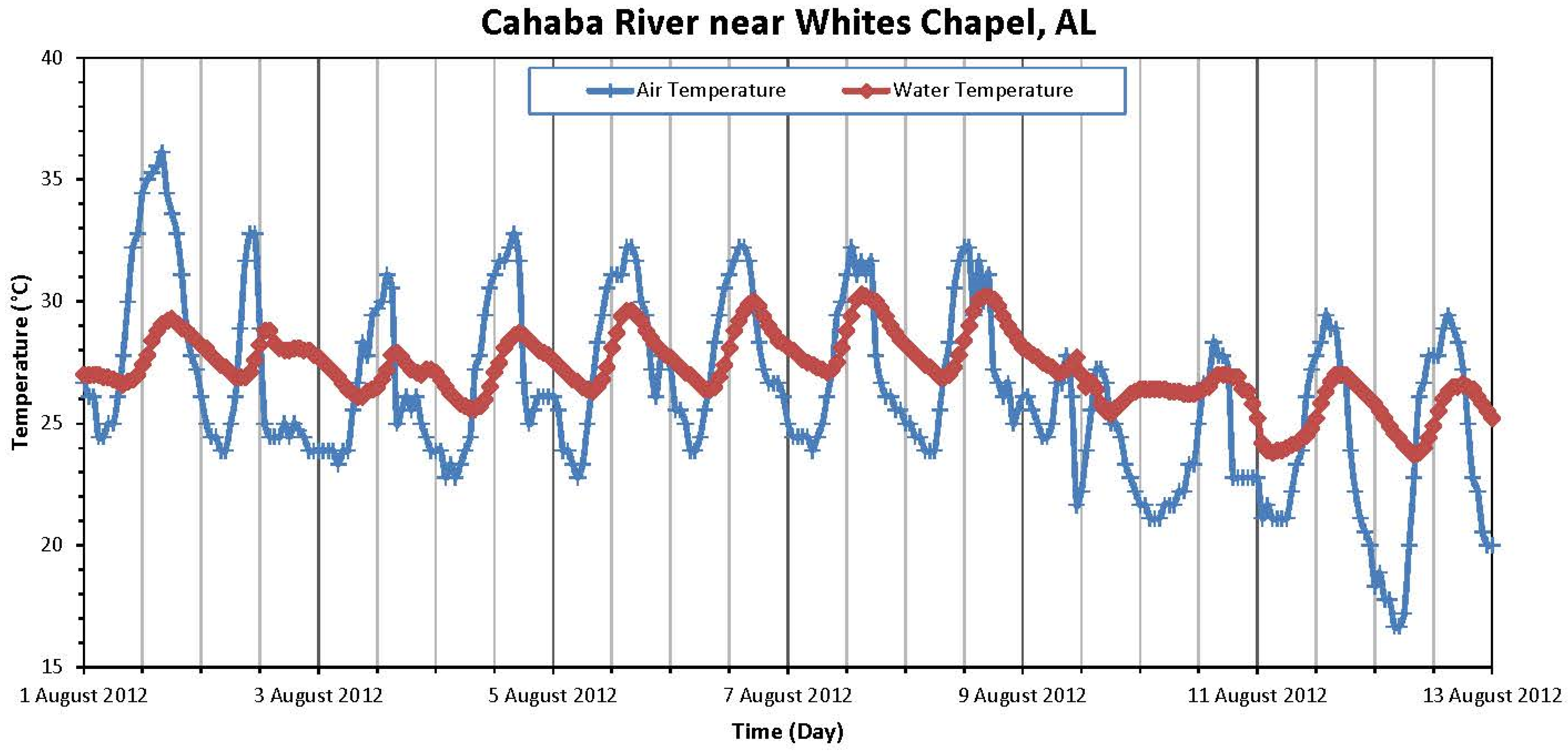
Figure 2 shows a time-series plot of hourly water temperature of the Cahaba River near Whites Chapel, and hourly air temperature at Birmingham International Airport (BHM, airport code) from 1 to 12 August 2012. The distance between two monitoring stations are 13.9 km. Figure 2 shows typical water temperature response to air temperature during the day and night. Water temperature variations have a lagged response behind air temperature fluctuations. For the Cahaba River near Whites Chapel, the lag was about 4 h. Therefore, lag time was used in the three regression models to investigate which model accuracy improvement the lag time can have.

Figure 2. Time-series of observed hourly water temperature of Cahaba River near Whites Chapel, AL and hourly air temperature at Birmingham International Airport from 1 to 12 August 2012.

Figure 2. Time-series of observed hourly water temperature of Cahaba River near Whites Chapel, AL and hourly air temperature at Birmingham International Airport from 1 to 12 August 2012.

Figure 3a,b show graphic examples of linear, polynomial and logistic regression models between hourly water temperatures in Cahaba River near Whites Chapel (abbreviated as Cahaba_Whites in Tables and Figures hereafter) and Sipsey Fork and hourly air temperatures at BHM. For these two rivers, a 4 h lag was incorporated for these regressions. For all eight streams, the linear regression models with time lags (4–5 h) are consistently but only slightly better than the regression model without time lag (Table 4). The NS improves by 0.01 at Coosa River and 0.06 at Sipsey Fork. The average improvement of RMSE for linear regression with time lag is about 0.3 °C (Table 4). Stefan and Preud’homme [13] had similar results of using lag times for regression models between daily water and air temperatures. They used a time lag, ranging from four hours to seven days depending on the depth of the stream and determined that introducing a lag time had an effect only for major rivers and improved the predictions by 0.5 °C or less.

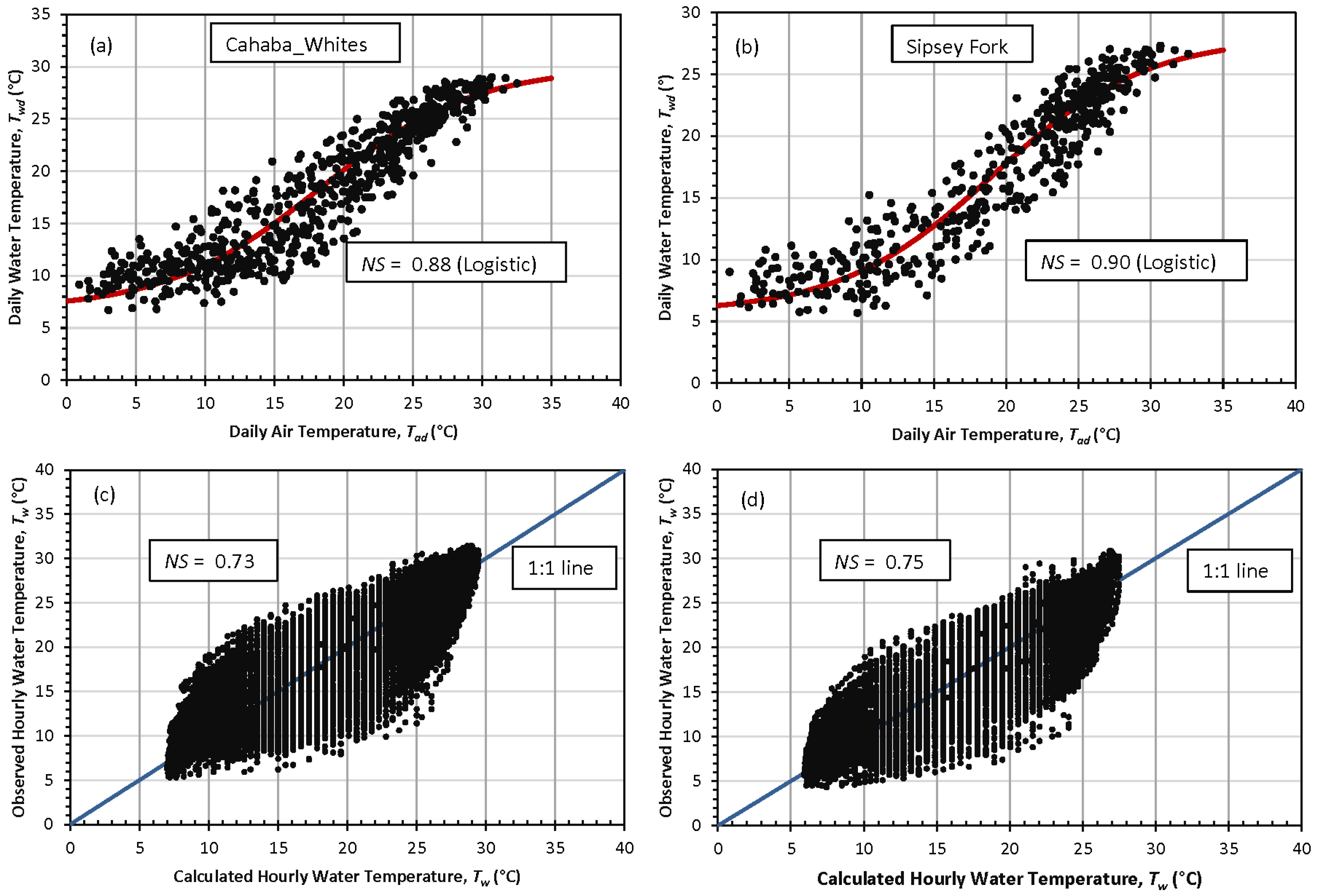
Figure 3. Hourly water−air temperature regressions of linear, polynomial and logistic models for (a) Cahaba River near Whites Chapel and (b) Sipsey Fork. Scatterplot for estimated hourly water temperatures from hourly logistic regression versus observed hourly water temperatures at (c) Cahaba River near Whites Chapel and (d) Sipsey Fork.

Figure 3. Hourly water−air temperature regressions of linear, polynomial and logistic models for (a) Cahaba River near Whites Chapel and (b) Sipsey Fork. Scatterplot for estimated hourly water temperatures from hourly logistic regression versus observed hourly water temperatures at (c) Cahaba River near Whites Chapel and (d) Sipsey Fork.

The physical interpretation of the water-air temperature relationship [26] shows that linear extrapolations to high and low air temperatures are not justified. Figure 3 shows that polynomial and logistic regression lines are closer to the data but depart from linear regression as air temperature exceeds 30 °C and falls below 5 °C in Cahaba River near Whites Chapel and Sipsey Fork. The logistic regression models fitted better to hourly data than the linear model did for high and low temperatures, and the polynomial regression models fitted better to hourly data for lower temperatures only (Figure 3).

Figure 3c,d show scatterplot for estimated hourly water temperatures from logistic regression models versus observed hourly water temperature in Cahaba River near Whites Chapel and Sipsey Fork. NS values are 0.79 and 0.82, respectively. Using time lag, the polynomial and logistic models for hourly water−air temperature regressions have slightly smaller MAE and RMSE and slightly larger NS, compared with linear regression models (Table 4). The average NS values of polynomial and logistic methods for eight rivers are both 0.76. The average MAE and RMSE are 2.7 and 3.3 °C for both methods. The NS for individual rivers improved only 0.01 or 0.02 from the linear model with time lag. MAE and RMSE decreased up to 0.16 and 0.13 °C, respectively. Therefore, the logistic models for eight rivers are only slightly better than the linear model and are the same as polynomial models, but regression parameters for logistic regression models have more meaningful interpretations. Further improvement of estimation from hourly air temperature to hourly water temperature is necessary.

3.2. Calculated Hourly Water Temperature from Daily Temperature Regression

Webb [43] observed that water-air temperature relationships become more scattered and less reliable as the time period over which the data are averaged becomes shorter. Studies have shown that as time scale increases (daily, weekly, monthly), the regression of water and air temperature improved significantly [6,9,13,29]. Therefore, logistic regression models between daily mean water and air temperatures were also developed for the eight rivers in AL. Figure 4a,b show graphic results of daily logistic regression models for two river stations. Daily regression models have smaller MAE and RMSE, and larger NS shown in Table 5 under the column “Mean-Temp” (numbers outside brackets) in comparison to statistical error parameters of hourly regression models shown in Table 4.

Figure 4. Daily water-air temperature regressions of logistic models in (a) Cahaba River near Whites Chapel and (b) Sipsey Fork. Scatterplot for estimated hourly water temperatures from daily logistic regression versus observed hourly water temperatures in (c) Cahaba River near Whites Chapel and (d) Sipsey Fork.

Figure 4. Daily water-air temperature regressions of logistic models in (a) Cahaba River near Whites Chapel and (b) Sipsey Fork. Scatterplot for estimated hourly water temperatures from daily logistic regression versus observed hourly water temperatures in (c) Cahaba River near Whites Chapel and (d) Sipsey Fork.

Before we discovered hourly observed water temperatures in eight rivers, the daily regression model from Pilgrim et al. [6] was used to estimate hourly water temperatures for small rivers to provide temperature boundary conditions for the 3-D EFDC modeling studies. What are model accuracies of using the daily regression models to estimate hourly water temperatures for each river? Figure 4c,d show two examples: Estimated hourly water temperatures from daily logistic regression models versus observed hourly water temperatures in Cahaba River near Whites Chapel and Sipsey Fork. NS for hourly estimations using daily regression models reduces from 0.88 (daily) to 0.73 (number inside brackets under “Mean-Temp” in Table 5) for Cahaba River near Whites Chapel and from 0.90 to 0.75 in Sipsey Fork. The same situation happened for all other rivers (Table 5) due to the daily mean air temperature not being able to reflect temperature fluctuation during the day and night. After comparing error parameters in Table 4 and Table 5 for hourly estimations using daily regression models NS values for eight rivers are only slightly smaller than NS values from direct hourly regression models (Table 4), and MAE and RMSE (Table 5) are only slightly larger. This shows that the hourly direct logistic models (Table 4) are not significantly better than daily regression models (Table 5) when they are used to estimate hourly water temperatures.

3.3. Calculated Hourly Water Temperature from Modified Wave Function Model

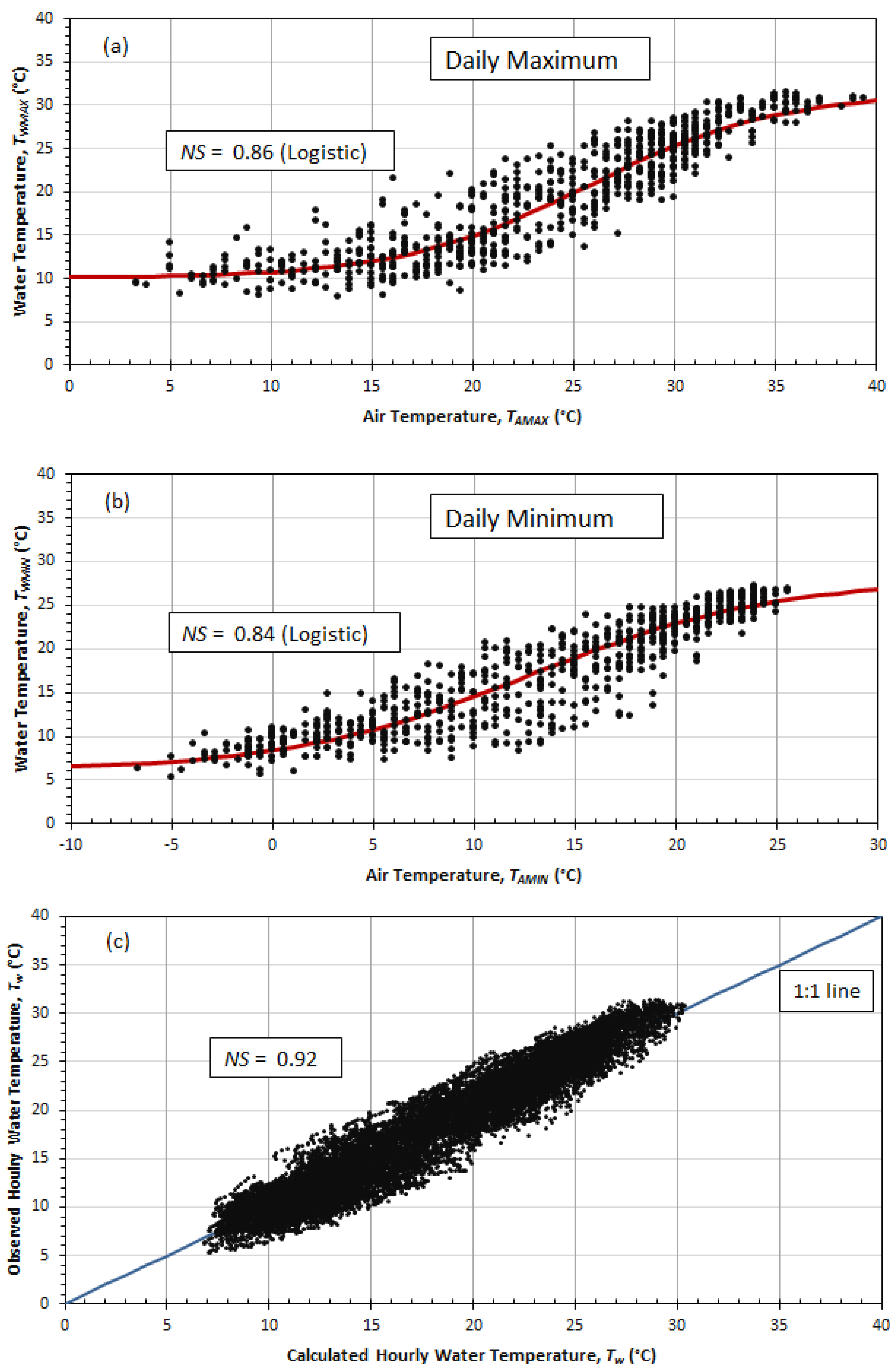
To improve model accuracy estimating hourly water temperatures, the modified WF model was investigated. Figure 5a,b show graphic results of logistic regression models between daily maximum and minimum water temperatures (T_WMAX and T_WMIN) in Cahaba River near Whites Chapel and daily maximum and minimum air temperatures (T_AMAX and T_AMIN) at BHM. T_WMAX and T_WMIN are input parameters for the modified WF model presented by Equations (4) and (5). The NS values for daily maximum and minimum temperature regression models range from 0.75 (Coosa) to 0.88 (Little Cahaba) and from 0.71 to 0.89, respectively, for eight Alabama rivers (Table 5). These NS values are larger than NS values for direct hourly regression models (Table 4).

Figure 5c shows a scatterplot for estimated hourly water temperatures from the modified WF model versus observed hourly water temperatures in Cahaba River near Whites Chapel. Comparing with Figure 3c and Figure 4c, data pairs on Figure 5c are much less scattered (closely distributed around 1:1 line). The NS is 0.92, that is, 0.15 larger than NS for the linear model with time lag in Cahaba River near Whites Chapel. Table 6 shows NS values for all eight rivers are all improved a lot by using the modified WF model. The NS values range from 0.83 at Coosa River to 0.93 at Little Cahaba (NS for most rivers exceeded 0.90). The average NS value for all rivers improved from 0.71 of the linear model to 0.89 of the modified WF model. The RMSE reduced from 3.58 to 2.18 °C. In summary, better performance of daily maximum and minimum temperature logistic regression models and the modified wave functions (Equations (4) and (5)) improved model accuracy in estimating hourly water temperatures in streams.

Figure 6a,b show a comparison of time-series estimated water temperatures by polynomial, logistic and modified WF models with observed water temperatures at Cahaba River near Whites Chapel and Sipsey Fork from 19 August to 29 August 2012. Figure 6 shows that direct polynomial and logistic models give less accurate estimates of lower temperatures from midnight to early morning. The modified WF models have overall better performance to estimate hourly water temperature in comparison to direct polynomial and logistic models.

Figure 7 shows that NS decreases with natural logarithm of the distance from BHM for all rivers except Sipsey Fork. Only Sipsey Fork has observed water temperatures for a one-year period. The other rivers have more than 2 years of data, and most of them have 5 or 6 years of data. Although the trend in Figure 7 is location dependent, it is what one would expect since only hourly air temperatures from BHM were used as input to estimate hourly water temperatures at all eight rivers. For NS ≥0.8 extrapolated from regression trendline equation, it seems that the distance from the air-temperature station should be less than 350 km. For more accurate estimate of hourly water temperature, using NS ≥0.9, the distance from the air-temperature station should be less than 30 km.

Figure 5. (a) Daily maximum and (b) daily minimum water-air temperature regressions using logistic model; and (c) Scatterplot for estimated hourly water temperatures from modified WF model versus observed hourly water temperatures in Cahaba River near Whites Chapel.

Figure 5. (a) Daily maximum and (b) daily minimum water-air temperature regressions using logistic model; and (c) Scatterplot for estimated hourly water temperatures from modified WF model versus observed hourly water temperatures in Cahaba River near Whites Chapel.

Figure 6. Comparison of time-series of estimated hourly water temperatures by polynomial, logistic and modified WF models with observed water temperatures at (a) Cahaba River near Whites Chapel from 19 August to 29 August 2012 and (b) Sipsey Fork from 30 July to 9 August 2012. NS values were calculated for all available data (see Table 1, not for above ten days).

Figure 6. Comparison of time-series of estimated hourly water temperatures by polynomial, logistic and modified WF models with observed water temperatures at (a) Cahaba River near Whites Chapel from 19 August to 29 August 2012 and (b) Sipsey Fork from 30 July to 9 August 2012. NS values were calculated for all available data (see Table 1, not for above ten days).

Figure 7. NS versus distance from the river temperature monitoring station to BHM (air temperature data station).

Figure 7. NS versus distance from the river temperature monitoring station to BHM (air temperature data station).

3.4. Calculated Hourly Water Temperature from Lumped Modified WF Model

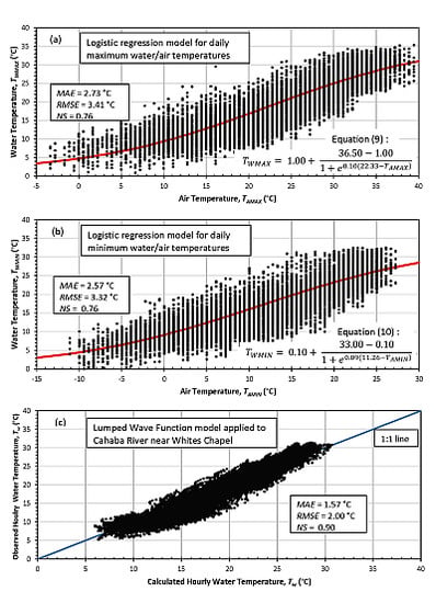
In this study, the modified WF model was first developed for each river (Table 5 and Table 6). Regression parameters of logistic models to estimate daily maximum and minimum water temperatures are listed in Table 7 for each river. The maximum and minimum water temperature data of eight rivers were also combined to develop two lumped logistic regression models (see graphic abstract) as follows:

$$T_{WMAX}=1.00+\frac{36.50-1.00}{1+e^{0.10(22.33-T_{AMAX})}}$$

(9)

$$T_{WMIN}=0.10+\frac{33.00-0.10}{1+e^{0.09(11.26-T_{AMIN})}}$$

(10)

Using Equations (9) and (10), the lumped WF model was applied to calculate hourly water temperatures for individual rivers (one example is shown in the graphic abstract). Table 6 shows that the lumped WF model has NS values ranged from 0.76 to 0.90 with average NS of 0.84, just slightly less than NS values from the modified WF models for individual rivers. The average RMSE is 2.64 °C, which is slightly larger than 2.18 °C, the average RMSE from individual WF models. In estimating hourly water temperatures, the lumped WF model still performs much better than direct hourly regression models, except for Little Cahaba and Sipsey Fork (similar performance).

Table 7. The parameters of logistic regression models for daily maximum and minimum water temperatures in eight rivers.

River	Daily Maximum Temperature				River	Daily Minimum Temperature
	α (°C)	β (°C)	γ	μ (°C)		α (°C)	β (°C)	γ	μ (°C)
Coosa	35.30	23.67	0.14	5.00	Coosa	32.50	12.11	0.13	4.20
Kelly	31.01	21.02	0.13	2.50	Kelly	29.50	9.53	0.12	1.20
Yellowleaf	33.93	22.89	0.12	2.00	Yellowleaf	28.86	10.07	0.11	0.10
Tallapoosa	32.50	23.11	0.13	6.80	Tallapoosa	31.00	11.67	0.11	5.00
Cahaba_Whites	31.50	25.76	0.21	10.00	Cahaba_Whites	27.00	12.76	0.17	6.00
Little Cahaba	27.80	21.02	0.13	7.80	Little Cahaba	25.40	8.97	0.11	4.00
Cahaba_Hoover	35.00	21.95	0.13	2.90	Cahaba_Hoover	31.50	10.21	0.12	1.20
Sipsey Fork	31.00	25.38	0.19	6.80	Sipsey Fork	26.50	13.29	0.16	4.40
Lumped All Rivers	36.50	22.33	0.10	1.00	Lumped All Rivers	33.00	11.26	0.09	0.10

Notes: α (^oC) is a coefficient that estimates maximum water temperature, μ (^oC) is a coefficient that estimates minimum water temperature, γ (dimensionless) represents the steepest slope (inflection point) of the logistic water temperature function when plotted against air temperature, and β (^oC) is air temperature at the inflection point. The bold parameters were developed using combined water temperature data from all rivers.

Table 7. The parameters of logistic regression models for daily maximum and minimum water temperatures in eight rivers.

River	Daily Maximum Temperature				River	Daily Minimum Temperature
	α (°C)	β (°C)	γ	μ (°C)		α (°C)	β (°C)	γ	μ (°C)
Coosa	35.30	23.67	0.14	5.00	Coosa	32.50	12.11	0.13	4.20
Kelly	31.01	21.02	0.13	2.50	Kelly	29.50	9.53	0.12	1.20
Yellowleaf	33.93	22.89	0.12	2.00	Yellowleaf	28.86	10.07	0.11	0.10
Tallapoosa	32.50	23.11	0.13	6.80	Tallapoosa	31.00	11.67	0.11	5.00
Cahaba_Whites	31.50	25.76	0.21	10.00	Cahaba_Whites	27.00	12.76	0.17	6.00
Little Cahaba	27.80	21.02	0.13	7.80	Little Cahaba	25.40	8.97	0.11	4.00
Cahaba_Hoover	35.00	21.95	0.13	2.90	Cahaba_Hoover	31.50	10.21	0.12	1.20
Sipsey Fork	31.00	25.38	0.19	6.80	Sipsey Fork	26.50	13.29	0.16	4.40
Lumped All Rivers	36.50	22.33	0.10	1.00	Lumped All Rivers	33.00	11.26	0.09	0.10

Notes: α (^oC) is a coefficient that estimates maximum water temperature, μ (^oC) is a coefficient that estimates minimum water temperature, γ (dimensionless) represents the steepest slope (inflection point) of the logistic water temperature function when plotted against air temperature, and β (^oC) is air temperature at the inflection point. The bold parameters were developed using combined water temperature data from all rivers.

Montgomery Regional Airport (Table 2) is relatively far away from most river monitoring stations (Figure 1). Tallapoosa River is the closest one, with a distance of just 25.4 km from Montgomery Regional Airport. Taking Tallapoosa River as an example, we redeveloped a modified WF model based on the air temperature data from Montgomery Regional Airport and recalculated the error parameters. The MAE, RMSE, and NS are 1.99 °C, 2.44 °C, and 0.84, respectively. The model accuracy at Tallapoosa River improves only a little bit: RMSE decreased 0.07 °C but there was no change of NS when using the air temperature data from Montgomery Regional Airport instead of BHM to develop the modified WF model (Table 6). Therefore, the modified WF models (both individual and lumped) based on BHM’s air temperatures will give us reasonably accurate hourly water temperature estimates for all rivers in Alabama. The lumped WF model (Equations (9) and (10), and Table 7) can be applied to other Alabama rivers when observed hourly temperatures are not available to develop a site-specific WF model.

4. Conclusions

This paper presents a modified WF model to estimate hourly water temperatures in rivers using daily maximum and minimum water temperatures as input. The logistic regression models were developed and used to estimate daily maximum and minimum water temperatures for the modified WF model from daily maximum and minimum air temperatures in each of eight rivers in Alabama, USA.

The direct linear and non-linear (polynomial and logistic) regression models were also developed to compare model accuracy in estimating hourly water temperatures with the modified WF model. These regression methods used a time lag of 4 to 5 h for eight rivers. Regression with time lag slightly improved hourly water temperature estimates without time lag. The results show significant improvement by using the modified WF model instead of direct regression models. The average NS value for eight rivers improved from 0.71 of the linear model to 0.89 of the modified WF model, and NS for the most rivers exceeded 0.90. The RMSE reduced from 3.58 °C to 2.18 °C. Figure 6 shows the modified WF models have overall better performance to estimate hourly water temperature in comparison to direct polynomial and logistic models.

A lumped WF model was also developed by combining all hourly water temperature data from all eight rivers. In estimating hourly water temperatures, the lumped WF model still performed much better than direct hourly regression models except for Little Cahaba and Sipsey Fork (similar performance). The lumped WF model had NS values ranging from 0.76 to 0.90 with average NS of 0.84, just slightly less than NS values from the modified WF models for individual rivers. The average RMSE is 2.64 °C that is slightly larger than 2.18 °C, the average RMSE from individual WF models. Therefore, the WF models (both individual and lumped) based on BHM’s air temperatures can be applied to give us reasonably accurate hourly water temperature estimates for all rivers in Alabama when observed hourly temperatures are not available to develop a site-specific WF model. The procedure to develop modified WF model can be applied to other regions.

References

- Caissie, D. The thermal regime of rivers: A review. Freshw. Biol. 2006, 51, 1389–1406. [Google Scholar]
- Coutant, C.C. Perspectives on Temperature in the Pacific Northwest’s Fresh Waters; Oak Ridge National Lab.: Oak Ridge, TN, USA, 1999. [Google Scholar]
- Johnson, M.; Wilby, R.; Toone, J. Inferring air—Water temperature relationships from river and catchment properties. Hydrol. Process. 2014, 28, 2912–2928. [Google Scholar]
- Schindler, D.W. The cumulative effects of climate warming and other human stresses on canadian freshwaters in the new millennium. Can. J. Fish. Aquat. Sci. 2001, 58, 18–29. [Google Scholar] [CrossRef]
- Sinokrot, B.; Stefan, H.G.; McCormick, M.J. Modeling of climate change effects on stream temperatures and fish habitats below dams and near groundwater inputs. Clim. Chang. 1995, 30, 181–200. [Google Scholar] [CrossRef]
- Pilgrim, J.M.; Fang, X.; Stefan, H.G. Stream temperature correlations with air temperatures in minnesota: Implications for climate warming. J. Am. Water Resour. Assoc. 1998, 34, 1109–1121. [Google Scholar] [CrossRef]
- Johnson, A.C.; Acreman, M.C.; Dunbar, M.J.; Feist, S.W.; Giacomello, A.M.; Gozlan, R.E.; Hinsley, S.A.; Ibbotson, A.T.; Jarvie, H.P.; Jones, J.I. The British river of the future: How climate change and human activity might affect two contrasting river ecosystems in england. Sci. Total Environ. 2009, 407, 4787–4798. [Google Scholar] [CrossRef] [PubMed]
- Erickson, T.R.; Stefan, H.G. Linear air/water temperature correlations for streams during open water periods. J. Hydrol. Eng. 2000, 5, 317–321. [Google Scholar] [CrossRef]
- Webb, B.; Clack, P.; Walling, D. Water—Air temperature relationships in a devon river system and the role of flow. Hydrol. Process. 2003, 17, 3069–3084. [Google Scholar] [CrossRef]
- Edinger, J.E.; Duttweiler, D.W.; Geyer, J.C. The response of water temperatures to meteorological conditions. Water Resour. Res. 1968, 4, 1137–1143. [Google Scholar] [CrossRef]
- Brown, G.W. An Improved Temperature Prediction Model for Small Streams; Water Resources Research Institute, Air Resources Center: Corvallis, OR, USA, 1972. [Google Scholar]
- Jobson, H.E. The dissipation of excess heat from water systems. J. Power Div. 1973, 99, 89–103. [Google Scholar]
- Stefan, H.G.; Preud’homme, E.B. Stream temperature estimation from air temperature. J. Am. Water Resour. Assoc. 1993, 29, 27–45. [Google Scholar] [CrossRef]
- Raphael, J.M. Prediction of temperature in rivers and reservoirs. J. Power Div. 1962, 88, 157. [Google Scholar]
- Brown, G.W. Predicting temperatures of small streams. Water Resour. Res. 1969, 5, 68–75. [Google Scholar] [CrossRef]
- Kothandaraman, V. Analysis of water temperature variations in large river. J. Sanit. Eng. Div. 1971, 97, 19–31. [Google Scholar]
- Cluis, D.A. Relationship between stream water temperature and ambient air temperature. Nord. Hydrol. 1972, 3, 65–71. [Google Scholar]
- Johnson, F. Stream temperatures in an alpine area. J. Hydrol. 1971, 14, 322–336. [Google Scholar] [CrossRef]
- Smith, K. The prediction of river water temperatures/prédiction des températures des eaux de rivière. Hydrol. Sci. J. 1981, 26, 19–32. (In French) [Google Scholar]
- Crisp, D. Water temperature in a stream gravel bed and implications for salmonid incubation. Freshw. Biol. 1990, 23, 601–612. [Google Scholar] [CrossRef]
- Crisp, D.; Howson, G. Effect of air temperature upon mean water temperature in streams in the North pennines and English lake district. Freshw. Biol. 1982, 12, 359–367. [Google Scholar] [CrossRef]
- Mackey, A.; Berrie, A. The prediction of water temperatures in chalk streams from air temperatures. Hydrobiologia 1991, 210, 183–189. [Google Scholar] [CrossRef]
- Webb, B.; Nobilis, F. Long-term perspective on the nature of the air-water temperature relationsihp: A case study. Hydrol. Process. 1997, 11, 137–147. [Google Scholar] [CrossRef]
- Caissie, D.; St-Hilaire, A.; El-Jabi, N. Prediction of Water Temperatures Using Regression and Stochastic Models; 57th Canadian Water Resources Association Annual Congress: Montreal, QC, Canada, 2004. [Google Scholar]
- Mohseni, O.; Stefan, H.G.; Erickson, T.R. A nonlinear regression model for weekly stream temperatures. Water Resour. Res. 1998, 34, 2685–2692. [Google Scholar] [CrossRef]
- Mohseni, O.; Stefan, H. Stream temperature/air temperature relationship: A physical interpretation. J. Hydrol. 1999, 218, 128–141. [Google Scholar] [CrossRef]
- Mohseni, O.; Stefan, H.G.; Eaton, J.G. Global warming and potential changes in fish habitat in US streams. Clim. Chang. 2003, 59, 389–409. [Google Scholar] [CrossRef]
- Morrill, J.C.; Bales, R.C.; Conklin, M.H. Estimating stream temperature from air temperature: Implications for future water quality. J. Environ. Eng. 2005, 131, 139–146. [Google Scholar] [CrossRef]
- Harvey, R.; Lye, L.; Khan, A.; Paterson, R. The influence of air temperature on water temperature and the concentration of dissolved oxygen in newfoundland rivers. Can. Water Resour. J. 2011, 36, 171–192. [Google Scholar] [CrossRef]
- Caissie, D.; El-Jabi, N.; St-Hilaire, A. Stochastic modelling of water temperatures in a small stream using air to water relations. Can. J. Civil Eng. 1998, 25, 250–260. [Google Scholar] [CrossRef]
- Morin, G.; Couillard, D. Predicting river temperatures with a hydrological model. Encycl. Fluid Mech. 1990, 10, 171–209. [Google Scholar]
- Sinokrot, B.; Stefan, H. Stream temperature dynamics: Measurements and modeling. Water Resour. Res. 1993, 29, 2299–2312. [Google Scholar]
- Cho, H.-Y.; Lee, K.-H. Development of an air–water temperature relationship model to predict climate-induced future water temperature in estuaries. J. Environ. Eng. 2011, 138, 570–577. [Google Scholar] [CrossRef]
- Chapra, S.C. Surface Water-Quality Modeling; Waveland Press: New York, NY, USA, 2008. [Google Scholar]
- Brunner, G.W. Hec-Ras River Analysis System: User’s Manual; US Army Corps of Engineers, Institute for Water Resources, Hydrologic Engineering Center: Davis, CA, USA, 2001. [Google Scholar]
- Cole, T.M.; Wells, S.A. CE-QUAL-W2: A two-dimensional, laerally averaged, hydrodynamic and water quality model, version 3.6 user manual. US Army Engineering and Research Development Center: Vicksburg, MS, USA, 2010. [Google Scholar]
- Craig, P.M. User’s manual for efdc_explorer 7: A pre/post processor for the environmental fluid dynamics code. Dynamic Solutions, LLC: Knoxville, TN, USA, 2012. [Google Scholar]
- Reicosky, D.; Winkelman, L.; Baker, J.; Baker, D. Accuracy of hourly air temperatures calculated from daily minima and maxima. Agric. For. Meteorol. 1989, 46, 193–209. [Google Scholar] [CrossRef]
- De Wit, C.T. Simulation of assimilation, respiration and transpiration of crops; Pudoc: Wageningen, The Netherlands, 1978. [Google Scholar]
- Hoogenboom, G.; Huck, M.G. Rootsimu v4. 0: A dynamic simulation of root growth, water uptake, and biomass partitioning in a soil-plant-atmosphere continuum: Update and documentation. In Agronomy and Soils Departmental Series-No. 109, Alabama Agricultural Experiment Station; Auburn University: Auburn, AL, USA, 1986. [Google Scholar]
- Chu, C.; Jones, N.E.; Piggott, A.R.; Buttle, J.M. Evaluation of a simple method to classify the thermal characteristics of streams using a nomogram of daily maximum air and water temperatures. N. Am. J. Fish. Manag. 2009, 29, 1605–1619. [Google Scholar] [CrossRef]
- Nash, J.E.; Sutcliffe, J.V. River flow forecasting through conceptual models part I—A discussion of principles. J. Hydrol. 1970, 10, 282–290. [Google Scholar] [CrossRef]
- Webb, B. Climate Change and the Thermal Regime of Rivers; University of Exeter: Exeter, South West England, UK, 1992. [Google Scholar]
© 2015 by the authors; licensee MDPI, Basel, Switzerland. This article is an open access article distributed under the terms and conditions of the Creative Commons Attribution license (http://creativecommons.org/licenses/by/4.0/).
Share and Cite
MDPI and ACS Style
Chen, G.; Fang, X. Accuracy of Hourly Water Temperatures in Rivers Calculated from Air Temperatures. Water 2015, 7, 1068-1087. https://doi.org/10.3390/w7031068
AMA Style
Chen G, Fang X. Accuracy of Hourly Water Temperatures in Rivers Calculated from Air Temperatures. Water. 2015; 7(3):1068-1087. https://doi.org/10.3390/w7031068
Chicago/Turabian StyleChen, Gang, and Xing Fang. 2015. "Accuracy of Hourly Water Temperatures in Rivers Calculated from Air Temperatures" Water 7, no. 3: 1068-1087. https://doi.org/10.3390/w7031068