Locating Leaks with TrustRank Algorithm Support

Abstract

This paper presents a methodology to quantify and to locate leaks. The original contribution is the use of a tool based on the TrustRank algorithm for the selection of nodes for pressure monitoring. The results from these methodologies presented here are: (I) A sensitivity analysis of the number of pressure transducers on the quality of the final solution; (II) A reduction of the number of pipes to be inspected; and (III) A focus on the problematic pipes which allows a better office planning of the inspection works to perform atthe field. To obtain these results, a methodology for the identification of probable leaky pipes and an estimate of their leakage flows is also presented. The potential of the methodology is illustrated with several case studies, considering different levels of water losses and different sets of pressure monitoring nodes. The results are discussed and the solutions obtained show the benefits of the developed methodologies.

1. Introduction

Water supply is one of the most valuable public services of civilized societies [1]. Water supply systems comprise two different parts: Transmission mains—pipes transporting water to tanks; and Water Distribution Networks (WDN)—pipes and service connections distributing water to costumers. However, these infrastructures are not completely watertight. Even in the most recent and well-built WDN, some level of leakage and occasional pipe bursts occur, leading to water losses.

Unlike in transmission mains, WDN are topologically complex and have service connections, making water loss control a difficult task. If the water lost is not visible or the consumers do not report service anomalies, such as low pressure or lack of water, leaks can be very difficult to locate. Leak location activity is usually supported by acoustic equipment, but this approach is expensive, requires specialized human labour and can be very time consuming. An automatic, quick and accurate leak location methodology or technique is the aspiration of every water company.

Although manufacturers continue developing new and better equipment, leak location in plastic pipes or in pipes with large diameters is still a problem. To contribute towards the mitigation of this problem, a new computational methodology was developed to help locating unreported leaks and estimating its flow (water loss assessment). This methodology results from linking a hydraulic simulation model to an optimization model. The hydraulic simulation model performs steady state analysis to estimate the water distribution network behaviour. The optimization model aims to minimize the difference between measured and estimated pressures, and its decision variables are the locations and flows from unreported leaks.

The success of methodologies based on pressure measurements is quite dependent on the number and location of the pressure transduces [2,3,4,5]. Thus, an innovative tool based on the TrustRank algorithm was developed to help selecting the nodes for pressure monitoring.

This paper presents a methodology to quantify and to locate leaks. The original contribution is the use of a tool based on the TrustRank algorithm for the selection of nodes for pressure monitoring. The results from these methodologies presented here are: (I) A sensitivity analysis of the number of pressure transducers on the quality of the final solution; (II) A reduction of the number of pipes to be inspected; and (III) A focus on the problematic pipes which allows a better office planning of the inspection works to perform atthe field. To obtain these results, a methodology for the identification of probable leaky pipes and an estimate of their leakage flows is also presented.

The potential of the methodology is illustrated with several case studies, considering different levels of water losses and different sets of pressure monitoring nodes. The results are discussed and the solutions obtained show the benefits of the developed methodologies.

State of the Art

According to Pilcher [6], in the 1850s water loss control in WDN was already a concern. Although these are fundamental infrastructures to communities, being buried, they often pass unnoticed to the public, and this distracts people’s awareness away from the water loss problem.

Water loss has several negative impacts, for both the water companies and the society itself, namely: operational (lower service level), economic (lower income and higher operating and capital costs), environmental (higher amount of water and energy usage, and consequent higher water and carbon footprints), public health (potential focus of contamination) and social (service disruptions, traffic disturbances and damage to people and their belongings). These impacts will be more severe with the increase of water demand, the climate change and water scarcity.

Water loss includes apparent losses (unauthorized consumption and customer meter inaccuracies) and real losses (leakage on transmission and/or distribution mains, leakage and overflows at utility’s storage tanks and leakage on service connections up to the point of customer metering). Real losses are an operational problem and correspond to the annual volume of water lost through leakage and overflows at tanks and leaks and bursts in pipes and service connections up to the point of customer metering [7].

The reduction of real losses in WDN can be attained by adopting active leakage control (ALC) policies. But ALC is not a simple task because unreported leaks can be very difficult to locate, in particular if the water lost is not visible or the customers do not report service anomalies (low pressure or lack of water). The leak location activity is usually supported by acoustic equipment, but it has some drawbacks: is quite expensive, requires specialized human labour, can be very time consuming and is not very effective in plastic pipes and pipes with large diameters. An automatic, quick and accurate leak location methodology or technique is the aspiration of every water company.

Monitoring is important in the water loss control context. Tank monitoring is the most common and usually comprises: water level (to avoid overflows and test for leakage) and flow, particularly during the night when consumption is at its minimum—minimum night flow (for real losses estimation and to support ALC activities). However, measurements in other parts of the WDN is also common, like flow measurement at the entrance of each district metered area (DMA) or pressure measurement at the entrance of each pressure management area (PMA) and at critical points [8]. Nevertheless, the opportunity to monitor pressure in other spots can play an important role in the context of WDN operation.

In the last few years the monitoring technology has undergone a remarkable evolution. Nowadays equipment is easily achievable, smaller, accurate and precise, can be battery powered and last for years, and can communicate through wireless networks. These new features contributed to widespread monitoring in WDN. Data collected through monitoring has been used for years to calibrate hydraulic models, and it is helpful in planning and operation activities, including leak location. But the location of the flow and pressure sensors plays an important role, and the optimal sensor placement is still an open research subject. For example, for leak location purposes, Candelieri et al. [9] selected the best locations by identifying the best trade-off between reliability and deployment costs, Bort et al. [10] compared two alternatives using pressure sensitivity; Blesa [11] used robustness analysis and clustering and Steffelbauer [12] investigated the use of Monte Carlo simulation.

Some of the existing methodologies developed for leak detection/location are based solely on the analysis of flow and/or pressure measurements: Artificial Neural Networks have been used for leak detection [13,14,15] and also for leak location [16]; Poulakis et al. [17] and Qi [18] proposed a Bayesian system identification methodology for leak location; Fuzzy Inference Systems, which are computational techniques from the field of Artificial Intelligence, were used by Mounce et al. [19] to detect leaks in WDN, and Fuzzy set theory was also used by Islam et al. [20] for leak detection and location; Aksela et al. [21] used self-organizing maps, combining flow data with a leak function to model leakages, to solve the leakage detection problem; Gertler et al. [22] applied principal component analysis to locate leaks; Jung et al. [23] used nonlinear Kalman filter; Okeya et al. used a modified Kalman filter [24]; Kang et al. [25] used control limit analysis to detect bursts; and Goulet et al. [5] used a model-falsification methodology for leak-detection.

Flow and/or pressure sensors data, combined with the energy and mass conservation laws, provide the necessary conditions to build state-estimation (or inverse) problems. This methodology was traditionally used to calibrate WDN models [26], given a set of flow and/or pressure measurements. Pudar and Liggett [27] presented a methodology based on this idea considering equivalent orifice areas of possible leaks as the unknowns. Andersen and Powell [28] presented an implicit formulation of the standard weighted least squares state-estimation problem, solved using an implicit Lagrangian approach. Poulakis et al. [17] used a Bayesian probabilistic framework to handle the unavoidable uncertainties in measurement and modeling errors, while Puust et al. [29] used the Shuffled Complex Evolution Metropolis (SCEM-UA) algorithm to estimate the probability density functions of unknown leak areas.

The same data combined with hydraulic simulation models can also be used to locate leaks in WDN. These hydraulic models can be based on steady state or unsteady state (transient) conditions. The arising of hydraulic transient based techniques to locate leaks occurred in the 1990s [30] and they consist inartificially introduce transients in the WDN and analyse the pressure data to locate the leaks. Despite that leak location with transients can be excellent for tank-pipe-tank systems, in real WDN its application can be much compromised. Due to the transients behaviour, the pressure data must be recorded with very short time steps and the accuracy of the procedure is very dependent on the celerity (pressure wave velocity), which can be difficult to estimate accurately in real world conditions. Notwithstanding, transient test-based techniques have proved to be effective in locating leaks in transmission mains. The pioneering work from Liggett and Chen [30] opened a new field of research. The main advances observed in the following two decades can be found in Colombo et al. [31] and Puust et al. [32] present extensive reviews of these methodologies. More recently signal processing has demonstrated its capabilities to help in this problem [33,34], the impedance method was used [35], wavelet analysis has improved [36,37], a portable pressure wave-maker has been designed [38] and experiments were carried out in real pipe systems to demonstrate the reliability of this approach [39,40].

Even knowing that true steady state conditions do not occur, leak location with steady state models seems to be a suitable approach for real world WDN [41]. The steady state based techniques simulate different hypothetical leakage scenarios, corresponding to different leak locations and severities (leak flows), trying to match the flow and/or pressure data obtained from transducers installed in the WDN. The implementation of this approach requires a calibrated model of the WDN and its accuracy depends on the pressure measurements and the head loss estimation. Leakage modelling can be performed using Demand-Driven-Analysis (DDA)—leak flows are pressure independent [42,43] or Pressure-Driven-Analysis (PDA)—leak flows depend on the pressure values [44,45], however, due to the pressure/leakage relationship, the latter approach is theoretically more sound. Wu and Sage [46] used DDA while Wu et al. [47] used PDA, but in both works the optimization problem to identify the leak locations was solved with genetic algorithms. Based on previous work [27,46], Ribeiro et al. [48] used a calibrated model and a simulated annealing algorithm to locate leaks during the minimum night flow period. The hydraulic simulations were performed assigning leak flows to pipes and these were equally distributed among the pipe endpoints. Solutions from this methodology helped to identify the most probable leak locations and estimate the respective leak flows.

As location and number of pressure transducers contribute to the success of methodologies to locate and quantify leaks, this paper presents an innovative tool based on the TrustRank algorithm to help in selecting the nodes for pressure monitoring.

2. Methodology

Firstly, a computational methodology was developed to help in locating unreported leaks and estimating its flow (water loss assessment). This methodology results from linking a hydraulic simulation model [49] to an optimization model [50]. The hydraulic simulation model performs steady state analysis to estimate the water distribution network behaviour. The optimization model aims to minimize the difference between measured and estimated pressures, and its decision variables are the locations and flows from multiple unreported leaks.

Secondly, a selection of the nodes to be monitored is made with an adaptation of the TrustRank algorithm and a sensitivity analysis to the number of pressure transducers on the quality of the final solution is evaluated. The results allow the identification of probable leaky pipes and an estimate of their leakage flow is also presented. Consequently, the pipes not identified in any solution have a reduced probability of having leaks. The results allow a better problem diagnosis and a supported planning of the inspection works to be performed at the field, with the number of pipes to be inspected considerably reduced.

2.1. Methodology for Identification of Probable Leaky Pipes and Estimation of Their Leak Flow

2.1.1. Link between Hydraulic Simulator and Optimization Model

Given a WDN with a certain total leakage flow, the methodology proposed here is intended to identify the most probable leaky pipes and estimate their leakage flows. It uses a calibrated model of the WDN to predict its hydraulic behaviour assuming that water consumption during the Minimum Night Flow period is known.

The WDN is being monitored (tanks are equipped with flow meters and a set of nodes is equipped with pressure transducers) and the information gathered in the past has been used to calibrate the model and the actual monitoring data will now be used to locate leaks.

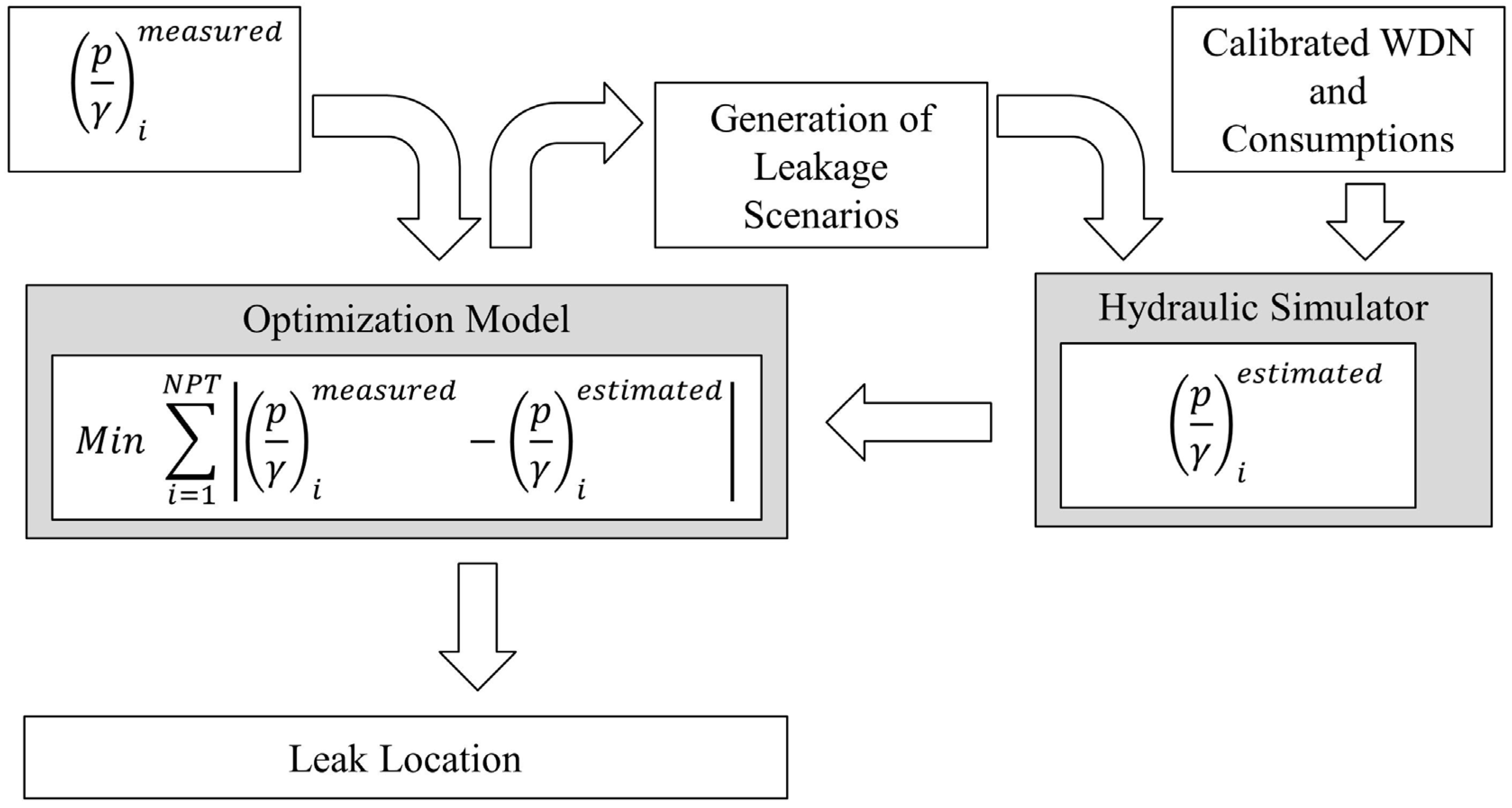
The leak location is achieved by simulating hypothetical leakage scenarios. The scenarios presenting pressure values close to those obtained from the field observations are selected. This is done by using an optimization model, which is solved by linking a simulated annealing algorithm with a hydraulic solver (Figure 1). The objective function is formulated to minimize the differences between measured (monitoring data) and estimated (simulation results) pressures.

Figure 1. Methodology to predict leak location and quantity.

Figure 1. Methodology to predict leak location and quantity.

2.1.2. Optimization Model

The objective function of the optimization model (1) is the minimization of the differences between the pressures measured “in situ” and the correspondent pressures estimated with the simulation model, for all monitored nodes:

$$MinF\left(x\right)=Min{\displaystyle \sum }_{i=1}^{NPT}\left|{\left(\frac{p}{\text{γ}}\right)}_i^{measured}-{\left(\frac{p}{\text{γ}}\right)}_i^{estimated}\right|$$

(1)

where: ${\left(\frac{p}{\text{γ}}\right)}_i^{measured}$= pressure head measured at node i (m); ${\left(\frac{p}{\text{γ}}\right)}_i^{estimated}$ = pressure head estimated at node i (m); γ = specific weight of water; NPT = number of nodes with pressure transducers.

The constraints of the optimization model are the common hydraulic constraints, like energy and continuity equations, and are implicitly tackled by the hydraulic simulation model.

2.1.3. Hydraulic Simulation Model

The WDN hydraulic behaviour is studied assuming steady state conditions, by using the mass and energy laws [51]. At the minimum night flow period water demand is usually very low and less uncertain. Head loss gets reduced and pressure head and leakage reach their maximum values. Although WDN hydraulic behaviour is always changing, under these conditions the steady state assumption does not introduce major inaccuracies [52]. For each leakage scenario, the hydraulic simulation model [49], compiled in FORTRAN, uses the node equations to estimate the pressure for the monitored nodes, under steady state conditions. These equations are solved by the Newton-Raphson method. This method has been successfully applied in several works [13,53,54,55], and here it is supported by a line search algorithm to optimize the step length in order to improve convergence and avoid the drawbacks of the original method. The node equations implicitly ensure the mass conservation and the energy laws, and the head losses were estimated with the Hazen-Williams Formula (2):

$$\text{Δ}{H}_{ij}=\mathrm{10.674.}\frac{L_{ij}.Q_{ij}^{1,852}}{CH{W}_{ij}^{1,852}.D_{ij}^{4,87}}$$

(2)

where: $\text{Δ}{H}_{ij}$ = head loss in the pipe between nodes i and j (m); $L_{ij}$ = length of the pipe between nodes i and j (m); $Q_{ij}$ = flow in the pipe between nodes i and j (m³/s); $D_{ij}$ = diameter of the pipe between nodes i and j (m);$CH{W}_{ij}$ = Hazen-Williams coefficient of the pipe between nodes i and j.

The Hazen-Williams formula is very simple and is widely used to estimate the friction losses from turbulent water flows in circular pipes at normal temperatures [27,56]. It was obtained empirically and is valid for pipes bigger than 50 mm and flow velocities under 3 m/s. Due to its simplicity and accuracy, since the beginning of the twentieth century this formula has been frequently used in the design and analysis of WDN.

2.1.4. Simulated Annealing Algorithm

The optimization model presented in Section 2.1.2 is non-linear, non-convex and contains continuous variables (leakage flow at each pipe), and so it was decided to use a simulated annealing algorithm [57,58] to solve it. Simulated annealing is a randomized search method [59] that is known to quickly find good solutions, even in extended search spaces. This method has been used to solve different problems from the water supply field, as documented in the literature: least cost design of WDN [60], robust design of WDN [61,62], optimal operation of WDN [63], optimal design and operation of WDN [55,64], pressure management in WDN [65], District Metered Areas design [66], and optimization of reservoir operation [67,68].

The simulated annealing method was inspired by the physical annealing process. The temperature is increased to a value considered high enough to melt a solid, following a slow cooling process in order to allow the molecular structure to reorganize and reach the minimum energy state—A crystal. Theoretically the algorithm converges to the global optimal solution [69] but in real world applications, due to the necessity to limit the number of solutions to evaluate, it is impossible to guarantee its global convergence. A simulated annealing algorithm requires the definition of an initial solution, an initial temperature, a procedure to build neighbourhoods, a cooling schedule (temperature decay and number of evaluations to be performed at each temperature), and a stopping criterion. The algorithm starts the search from an initial solution, which at this stage also plays the roles of best solution found so far and current solution. Then the neighbourhood procedure is used to identify a candidate solution in the neighbourhood of the current solution. The hydraulic behaviour of this candidate solution is estimated with the hydraulic simulation model, and its quality is assessed by the objective function (1). The acceptance or rejection of each candidate solution is governed by the Metropolis criterion (if the candidate solution is better than the current solution it is accepted, otherwise it may be accepted with a certain probability). The algorithm implemented comprises the following steps and the information presented in Table 1:

Table 1. Simulated annealing algorithm implementation.

Part of the algorithm	Implementation
Initial solution (x0)	The total leakage flow is split and each part is assigned to a selected pipe
Initial temperature (Tqt_initial)	Tqt_initial = −0.1 × F(x0)/Log(0.5)
Cooling schedule	If Pa > 80% Tqti+1 = 0.60 × Tqti	IAi+1 = 40
	If Pa > 50% Tqti+1 = 0.75 × Tqti	IAi+1 =60
	If Pa > 20% Tqti+1 = 0.90 × Tqti	IAi+1 =80
	If Pa ≤ 20% Tqti+1 = 0.95 × Tqti	IAi+1 =100
Number of evaluations at each temperature Tqti	IAi × Number of pipes in the network
Stopping criteria	Pa < 5% and 2 temperatures without solution improvement

Table 1. Simulated annealing algorithm implementation.

Part of the algorithm	Implementation
Initial solution (x0)	The total leakage flow is split and each part is assigned to a selected pipe
Initial temperature (Tqt_initial)	Tqt_initial = −0.1 × F(x0)/Log(0.5)
Cooling schedule	If Pa > 80% Tqti+1 = 0.60 × Tqti	IAi+1 = 40
	If Pa > 50% Tqti+1 = 0.75 × Tqti	IAi+1 =60
	If Pa > 20% Tqti+1 = 0.90 × Tqti	IAi+1 =80
	If Pa ≤ 20% Tqti+1 = 0.95 × Tqti	IAi+1 =100
Number of evaluations at each temperature Tqti	IAi × Number of pipes in the network
Stopping criteria	Pa < 5% and 2 temperatures without solution improvement

Step 1: Choose the initial solution (x₀), the initial temperature (Tqt_initial) and fix the number of solutions to be evaluated at each temperature (IA multiplied by the number of pipes in the WDN). The initial solution assumes the roles of current solution (x_current) and best solution found so far (x_best);

Step 2: Generate a candidate solution accessible from the current solution (x_candidate) by applying one of the next two processes: (I) Transfer an elementary unit of the leakage flow from one pipe to one of its adjacent pipes (diversification mechanism); (II) Randomly select a leaky pipe and concentrate in it all the leaks from its adjacent pipes (concentration mechanism);

Step 3: Check the hydraulic behaviour of the candidate solution and assess the solution quality with the objective function (1);

Step 4: Apply the Metropolis criterion: If the candidate solution is better than the current solution or fulfils the condition established in Equation (3) it is accepted and becomes the next current solution (if this candidate solution is better than the best solution found so far, it takes its place), otherwise the candidate solution is rejected and the current solution is maintained:

$$randomnumber<exp\left(-\frac{F_{(x_{current})}-F_{(x_{candidate})}}{Tq{t}_i}\right)$$

(3)

Step 5: Increment the counter of solutions evaluated at this temperature. If this counter does not exceed the number of solutions to be evaluated at this temperature, go to Step 2;

Step 6: Apply the cooling schedule (Table 1) that defines the temperature decrease (Tqt_i+1) and the number of solutions to be evaluated at the new temperature as a function of the percentage of accepted solutions (Pa) at the previous temperature (Tqt_i);

Step 7: If the stopping criteria is not met, restart the counter of solutions evaluated at the new temperature and return to Step 2, otherwise stop and the final solution is x_best.

2.2. Methodology for Pressure Transducers Location

In the context of leak location in WDN, fixing the adequate number of pressure transducers and its optimal placement is not an easy task. They are expensive and there are no simple rules to define the number of pressure transducers as a function of the WDN characteristics (for example, based on the length, total flow or leakage flow). If the WDN is divided in DMAs, it is common to install at least one pressure transducer at the critical node of each DMA (node with minimum pressure closer to the minimum required), and if the DMA is also a PMA it may also include a pressure transducer at the entrance node.

On the other hand, in networks without DMAs, to obtain a good coverage of the entire WDN, the spots where to install pressure transducers depend on their quantity and different quantities will certainly lead to different placements. It is known that all these variables can be interrelated and constrain the optimal solution [3].

The cost of acquiring the pressure transducers and gathering data limits the number of nodes to be monitored. In theory, if data was collected at all nodes, the methodology proposed here would certainly identify correctly all the leaks. In a previous paper [48], an attempt was made assuming that all end nodes of branched pipes were monitored and the methodology produced promising results. However, in real WDN there are usually also space and functional limitations for placing pressure transducers. Being so, this paper presents a methodology for pressure transducers location and a sensitivity analysis of the impact of increasing the number of pressure transducers on the quality of the final solution.

Adaptation of the TrustRank Algorithm to Water Distribution Networks (WDN)

The selection of the nodes to be monitored is made with an adaptation of the TrustRank algorithm for WDN. The TrustRank algorithm [70] was originally developed to separate the good web pages from bad (spam) and it is used by internet search engines. For every webpage, the algorithm assigns a trust score. The foundations of the algorithm for assigning the trust score are: a good page has high trust score and rarely points to bad pages (“approximate isolation of the good set”); In the transition from one web page to another there is transmission of trust, and trust reduces as we move away from the good pages (“trust attenuation”). The trust transmitted from a webpage (source) to the following (destination) is inversely proportional to the number of links from the source page (“trust splitting”).

The adaptation of the TrustRank algorithm to WDN is straightforward. Based on the water demand, this algorithm can easily select the nodes where the uncertainty of the pressure head is higher. In WDN all nodes are connected by pipes and the water flows from the source nodes (reservoirs/tanks) to the junction nodes downstream. Thus, the nodes of the WDN can be organized in a way similar to the web pages. The adapted trust transmission law is represented by Equation (4):

$$T\left(d\right)=\frac{R(s)}{N}$$

(4)

where, T(d) = trust transmission of the source node (s) to the destination node (d); R(s) = trust score of the source node; N = number of pipes that discharge from node (s).

Reservoirs/tanks are the nodes with the highest trust scores (1.0). They are sources, the most influential nodes [71], this means, nodes where the water level is known as well as the total flow (demand and leakage) is provided and measured. At the minimum night flow period, the hydraulic simulator is used to calculate flows in pipes, and this flow pattern rules the order of the trust transmission law.

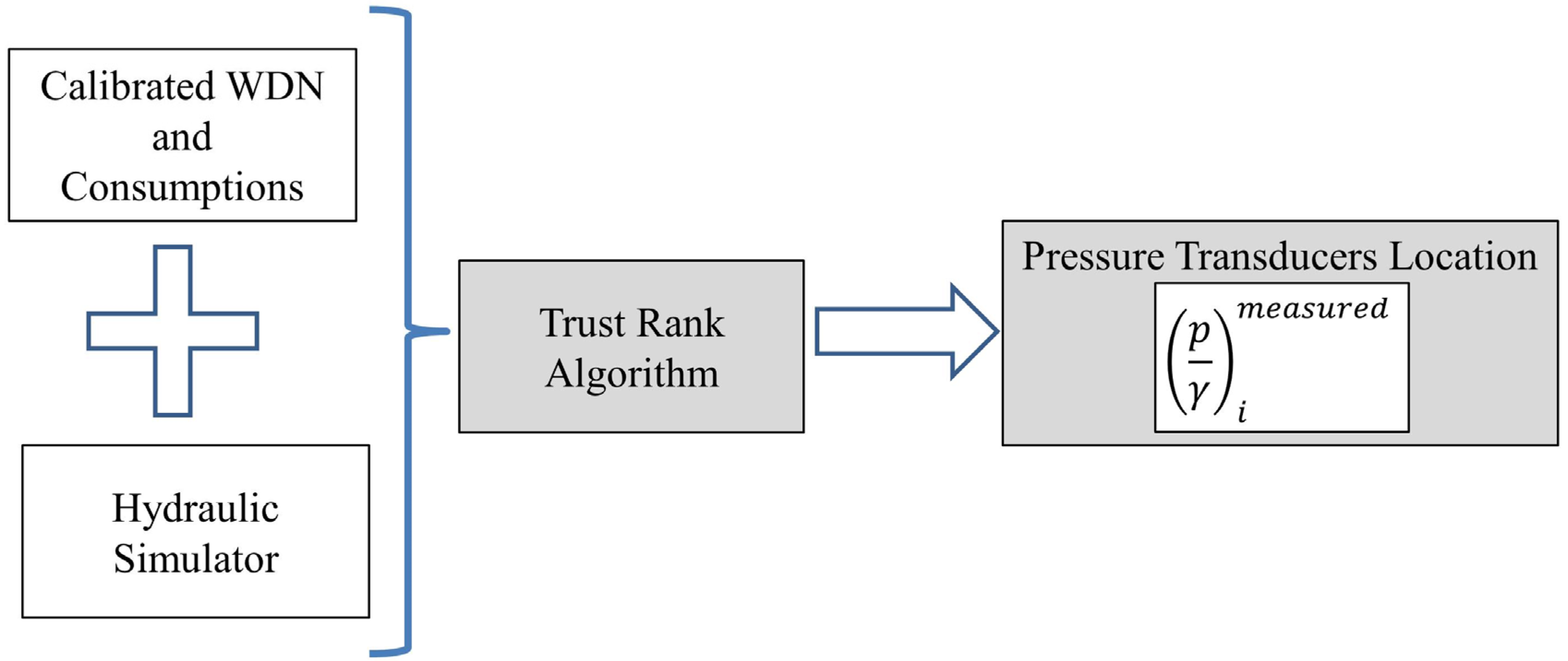
The trust score of a junction node is the sum of the trust transmissions from all the nodes that supply it (closest upstream nodes). In pipes with a flow below the stop criterion of the hydraulic simulator (head loss close to zero), it is assumed that there is no reliable trust transmission. Endpoints with the lowest trust scores are the first to be monitored because they are the less influential nodes (nodes with higher uncertainty and the transducers information will serve to reduce it). If the number of nodes with equal trust score exceeds the number of points to be monitored, the pressure transducers are randomly placed in those nodes (Figure 2).

Figure 2. Methodology for selection of pressure transducers placement.

Figure 2. Methodology for selection of pressure transducers placement.

2.3. Computer Application

The methodology described below was implemented as a computer application with a user interface to facilitate the communication between the user and the different modules. It assumes that there is a calibrated model of the WDN, actual total leakage flow can be estimated by comparing the actual minimum night flow with historical data or by estimating the minimum night consumption and subtracting it to the actual minimum night flow. The hydraulic simulation model has a stop criterion of one centimetre in pressure and one centilitre per second in flow. Taking into account the hydraulic simulation model and the pressure sensors accuracies, the pressure measurements were truncated at the millimetre.

The procedure starts by dividing the total leakage flow in a user defined number of flow units and the result is the elementary unit of leakage flow (Δql).

The construction of the initial solution (x₀) starts by assigning the water consumption to the junction nodes. Then, sequentially, each Δql is assigned to a pipe using the following procedure: assign one Δql to one of the pipes in the network (a half of each elementary unit of leakage flow is assigned to its end nodes), use the hydraulic simulation model to simulate the hydraulic behaviour of the WDN (considering both water consumption and leakage—Δql already assigned), assess the objective function (1), repeat the simulation for each of the pipes in the network and finally assign this Δql to the pipe that obtained the lowest value of the objective function (1); Repeat the process until all Δql are assigned. At this stage the total leakage flow is completely assigned (note that some pipes may have more than one Δql) and this is the initial solution to start solving the optimization model. The objective function value of the initial solution (F(x₀)) is then used to calculate the initial temperature (Tqt_initial) to start the simulated annealing algorithm.

Due to the stochastic nature of the simulated annealing algorithm, the robustness of the search process was tested by solving the optimization problem with fifty different sets of random numbers (different seeds). The search procedure evolves by generating different combinations of leakage flows assigned to pipes (candidate solutions) looking for the one that best fits the pressure measurements. Each set of random numbers produces one solution (if the search procedure is robust these solutions should be equal or, at least, similar) and at the end the methodology builds the final solution by combining the fifty solutions, identifying for each pipe the number of times that it was part of a solution. Pipes figuring more times in the fifty solutions are potential leaky pipes—greater probability of having leaks, while pipes that were not identified have zero probability of being leaky pipes.

3. Results

3.1. Case Study

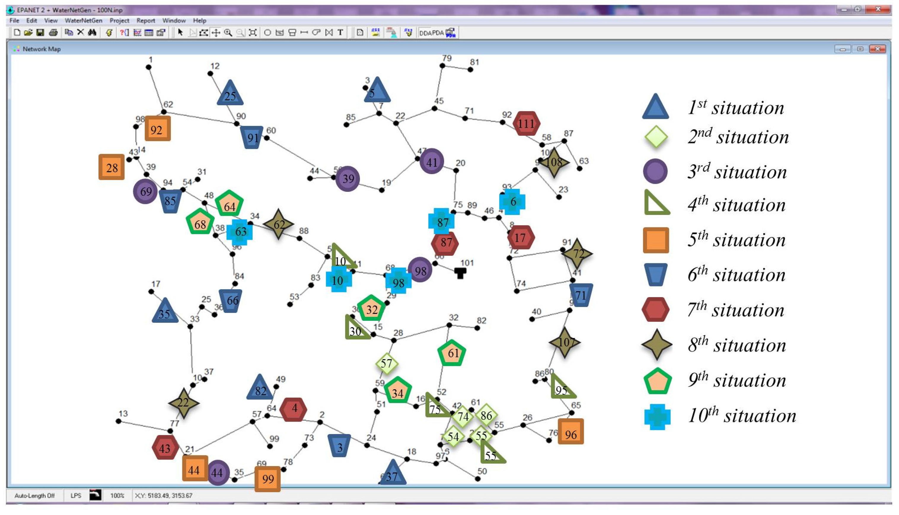
The performance of the proposed methodology is illustrated with 240 case studies created specifically for that purpose. All the case studies use the same WDN (one tank, 100 junction nodes, 111 pipes and 11 loops), but considering two different lengths (each pipe has its original length—first WDN, and half—second WDN), two leakage flow scenarios (1.5 and 15.0 L/s), 10 random spatial distributions of the leakage flows (situations presented in Table 2 and illustrated in Figure 3) and collecting data from six different sets of monitoring nodes (10, 12, 14, 16, 18 and 20 pressure transducers).

Table 2. Leakage flow spatial distributions (situations) for scenario 1 (1.5 L/s).

Situations—Pipe/Leakage Flow (L/s)
1	2	3	4	5	6	7	8	9	10
5/0.5	54/0.1	39/0.1	10/0.1	28/0.1	3/0.5	4/0.1	22/0.1	32/0.1	6/0.5
25/0.3	55/0.2	41/0.2	30/0.2	44/0.2	66/0.3	17/0.2	62/0.2	34/0.2	10/0.2
35/0.4	57/0.5	44/0.4	55/0.3	92/0.4	71/0.4	43/0.5	72/0.4	61/0.3	63/0.1
37/0.2	74/0.3	69/0.5	75/0.4	96/0.5	85/0.2	87/0.3	107/0.5	64/0.5	87/0.4
82/0.1	86/0.4	98/0.3	95/0.5	99/0.3	91/0.1	111/0.4	108/0.3	68/0.4	98/0.3

Table 2. Leakage flow spatial distributions (situations) for scenario 1 (1.5 L/s).

Situations—Pipe/Leakage Flow (L/s)
1	2	3	4	5	6	7	8	9	10
5/0.5	54/0.1	39/0.1	10/0.1	28/0.1	3/0.5	4/0.1	22/0.1	32/0.1	6/0.5
25/0.3	55/0.2	41/0.2	30/0.2	44/0.2	66/0.3	17/0.2	62/0.2	34/0.2	10/0.2
35/0.4	57/0.5	44/0.4	55/0.3	92/0.4	71/0.4	43/0.5	72/0.4	61/0.3	63/0.1
37/0.2	74/0.3	69/0.5	75/0.4	96/0.5	85/0.2	87/0.3	107/0.5	64/0.5	87/0.4
82/0.1	86/0.4	98/0.3	95/0.5	99/0.3	91/0.1	111/0.4	108/0.3	68/0.4	98/0.3

Figure 3. Network layout with ten situations (leakage flow spatial distributions).

Figure 3. Network layout with ten situations (leakage flow spatial distributions).

The use of the same WDN with different lengths is intended to assess the methodology performance under the influence of different head losses.

The original length of the WDN is almost forty-three kilometres (42.935 km) and during the minimum night flow period the water consumption equals 2.315 L/s. For each situation the leaky pipes were randomly chosen and the leakage flows range from 0.1 to 0.5 L/s in scenario 1 (Table 2) and for scenario 2 the leakage flows are ten times those from scenario 1 in the same pipe.

3.2. TrustRank Algorithm Application

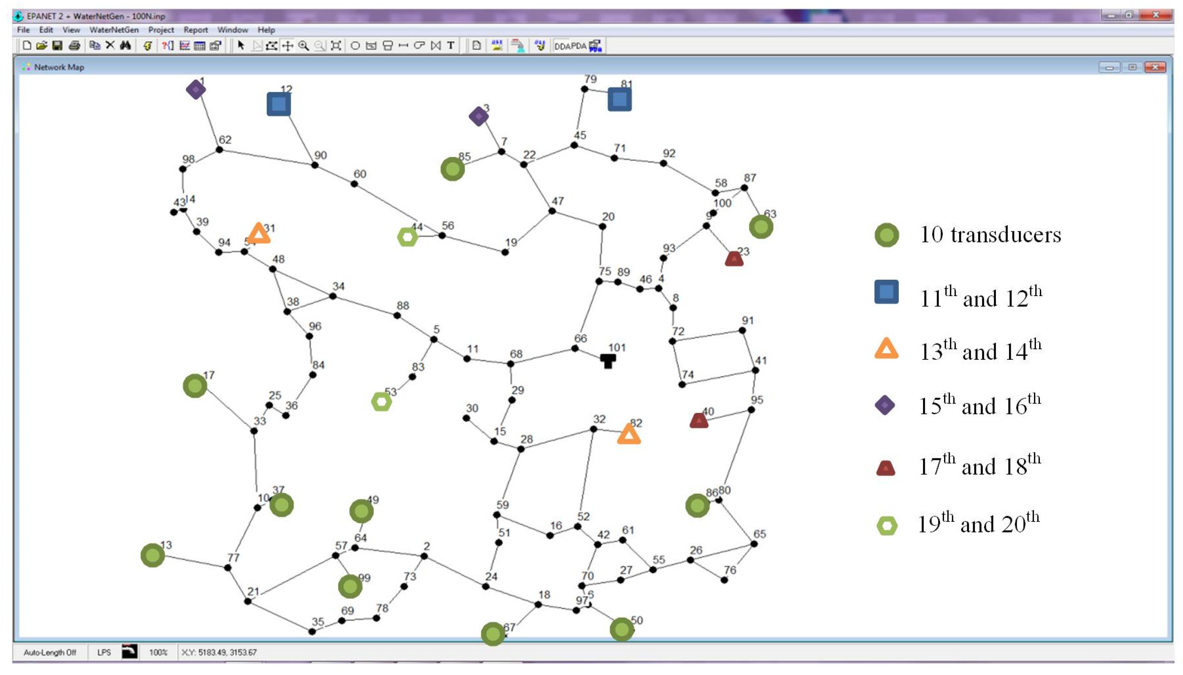
The results from the TrustRank algorithm (trust score for each node) are presented in

Table A1. Node trust scores.

Node	Trust Score	Node	Trust Score	Node	Trust Score
1	0.04688	35	0.00781	69	0.00781
2	0.01563	36	0.06250	70	0.03125
3	0.03125	37	0.01565	71	0.06250
4	0.25000	38	0.06250	72	0.12500
5	0.25000	39	0.03125	73	0.00781
6	0.02344	40	0.06250	74	0.06250
7	0.06250	41	0.12500	75	0.50000
8	0.12500	42	0.06250	76	0.07813
9	0.12500	43	0.01563	77	0.02734
10	0.03125	44	0.06250	78	0.00781
11	0.25000	45	0.06250	79	0.03125
12	0.03125	46	0.25000	80	0.06250
13	0.02734	47	0.25000	81	0.03125
14	0.03125	48	0.06250	82	0.03125
15	0.25000	49	0.00391	83	0.12500
16	0.03125	50	0.02344	84	0.06250
17	0.03125	51	0.03125	85	0.03125
18	0.01563	52	0.06250	86	0.03125
19	0.12500	53	0.12500	87	0.06250
20	0.25000	54	0.06250	88	0.12500
21	0.01172	55	0.04688	89	0.25000
22	0.12500	56	0.12500	90	0.06250
23	0.06250	57	0.00781	91	0.06250
24	0.03125	58	0.03125	92	0.03125
25	0.06250	59	0.06250	93	0.12500
26	0.04688	60	0.06250	94	0.03125
27	0.01563	61	0.03125	95	0.12500
28	0.12500	62	0.04688	96	0.06250
29	0.25000	63	0.03125	97	0.00781
30	0.12500	64	0.00781	98	0.01563
31	0.03125	65	0.03125	99	0.00195
32	0.06250	66	1.00000	100	0.06250
33	0.06250	67	0.00781	101	1.00000
34	0.12500	68	0.50000	–	–

(Appendix), in which the first ten nodes with pressure transducers are in bold. Each of the six sets of monitoring nodes (pressure transducer placement) is presented in Table 3 and illustrated in Figure 4. The sets of monitoring nodes represent from 10% up to 20% of the nodes in the WDN.

Table 3. Pressure transducer placement.

Transducers	Placement (Nodes)
First 10	13, 17, 37, 49, 50, 63, 67, 85, 86, 99
11th and 12th	12, 81
13th and 14th	31, 82
15th and 16th	1, 3
17th and 18th	23, 40
19th and 20th	44, 53

Table 3. Pressure transducer placement.

Transducers	Placement (Nodes)
First 10	13, 17, 37, 49, 50, 63, 67, 85, 86, 99
11th and 12th	12, 81
13th and 14th	31, 82
15th and 16th	1, 3
17th and 18th	23, 40
19th and 20th	44, 53

Figure 4. Network layout with the pressure transducers placement.

Figure 4. Network layout with the pressure transducers placement.

As previously mentioned, the methodology starts by calculating fifty solutions, obtained with different sets of random numbers, and builds the final solution afterwards in which each pipe is represented by the number of times it was identified as a probable leaky pipe in those solutions. To facilitate the analysis, results are presented in the format of reliable leaky pipes (those that were identified at least ten times, that is, in 20% of the solutions) and total leaky pipes (those that were identified at least once).

3.3. Sensitivity Analysis of the Number of Pressure Transducers

3.3.1. First WDN

The total length of the first WDN is 42.935 km (each pipe presents its original length). During the minimum night flow, if there was no leakage (only 2.315 L/s of water consumption), the head loss between the tank (node 101) and the hydraulically furthest node (node 13) is 0.039 m. Results from the proposed methodology (number of reliable and total leaky pipes) are presented in Table 4 and Table 5, where the crossing of the situation (horizontally) with the number of pressure transducers (vertically) leads to the number of reliable and total leaky pipes for scenarios 1 (Sc1) and 2 (Sc2).

Table 4. Number of reliable leaky pipes in the first WDN (scenario 1/scenario 2).

Situation	Number of Pressure Transducers
	10	12	14	16	18	20
1	7/5	7/5	7/5	5/5	5/5	5/5
2	14/5	14/5	6/5	6/5	7/5	10/5
3	18/6	10/6	12/5	12/5	8/5	8/5
4	16/14	13/16	11/9	12/9	12/9	17/9
5	11/5	9/5	8/5	7/5	7/5	7/5
6	19/7	14/6	15/12	12/5	5/5	5/5
7	17/5	9/5	8/5	7/5	8/5	8/5
8	16/5	14/5	13/5	9/5	6/5	6/5
9	13/12	17/11	16/7	15/7	16/7	10/7
10	19/11	12/5	11/5	9/5	12/5	10/5

Table 4. Number of reliable leaky pipes in the first WDN (scenario 1/scenario 2).

Situation	Number of Pressure Transducers
	10	12	14	16	18	20
1	7/5	7/5	7/5	5/5	5/5	5/5
2	14/5	14/5	6/5	6/5	7/5	10/5
3	18/6	10/6	12/5	12/5	8/5	8/5
4	16/14	13/16	11/9	12/9	12/9	17/9
5	11/5	9/5	8/5	7/5	7/5	7/5
6	19/7	14/6	15/12	12/5	5/5	5/5
7	17/5	9/5	8/5	7/5	8/5	8/5
8	16/5	14/5	13/5	9/5	6/5	6/5
9	13/12	17/11	16/7	15/7	16/7	10/7
10	19/11	12/5	11/5	9/5	12/5	10/5

Table 5. Number of total leaky pipes in the first WDN (scenario 1/scenario 2).

Situation	Number of Pressure Transducers
	10	12	14	16	18	20
1	7/5	7/5	7/5	5/5	5/5	5/5
2	24/19	26/17	24/9	18/9	20/5	22/11
3	36/24	31/27	16/5	12/5	10/5	8/5
4	31/25	28/25	18/14	20/11	22/17	23/14
5	34/5	14/5	8/5	12/5	11/5	11/5
6	68/45	47/28	50/30	32/25	18/7	5/5
7	49/34	21/6	8/6	7/5	11/5	12/5
8	32/5	27/5	20/5	20/5	6/5	6/5
9	42/34	45/35	33/13	26/16	25/9	19/7
10	63/54	46/38	21/30	22/24	20/5	14/5

Table 5. Number of total leaky pipes in the first WDN (scenario 1/scenario 2).

Situation	Number of Pressure Transducers
	10	12	14	16	18	20
1	7/5	7/5	7/5	5/5	5/5	5/5
2	24/19	26/17	24/9	18/9	20/5	22/11
3	36/24	31/27	16/5	12/5	10/5	8/5
4	31/25	28/25	18/14	20/11	22/17	23/14
5	34/5	14/5	8/5	12/5	11/5	11/5
6	68/45	47/28	50/30	32/25	18/7	5/5
7	49/34	21/6	8/6	7/5	11/5	12/5
8	32/5	27/5	20/5	20/5	6/5	6/5
9	42/34	45/35	33/13	26/16	25/9	19/7
10	63/54	46/38	21/30	22/24	20/5	14/5

For leakage scenario 1 (Sc1), situation 1 (St1) described in Table 2 (identification of the leaky pipes and respective leak flows), and using the first transducers set described in Table 3, seven pipes were identified as reliable leaky pipes (first number in the cell defined by row “Situation 1” and column “Number of pressure transducers 10” in Table 4). The same pipes were identified as total leaky pipes (first number in the cell defined by row ”Situation 1” and column “Number of pressure transducers 10” in Table 5). Five from these seven pipes were precisely the correct leaky pipes presented in Table 2.

For leakage scenario 2 (Sc2), situation 1 (St1) described in Table 2 (identification of the leaky pipes and the respective leak flows are ten times the leak flows presented), and using the first transducers set described in Table 3, five pipes were identified as reliable leaky pipes (second number in the cell defined by row “Situation 1” and column “Number of pressure transducers 10” in Table 4), as well as total leaky pipes (second number in the cell defined by row “Situation 1” and column “Number of pressure transducers 10” in Table 5). These five pipes were precisely the correct leaky pipes presented in Table 2.

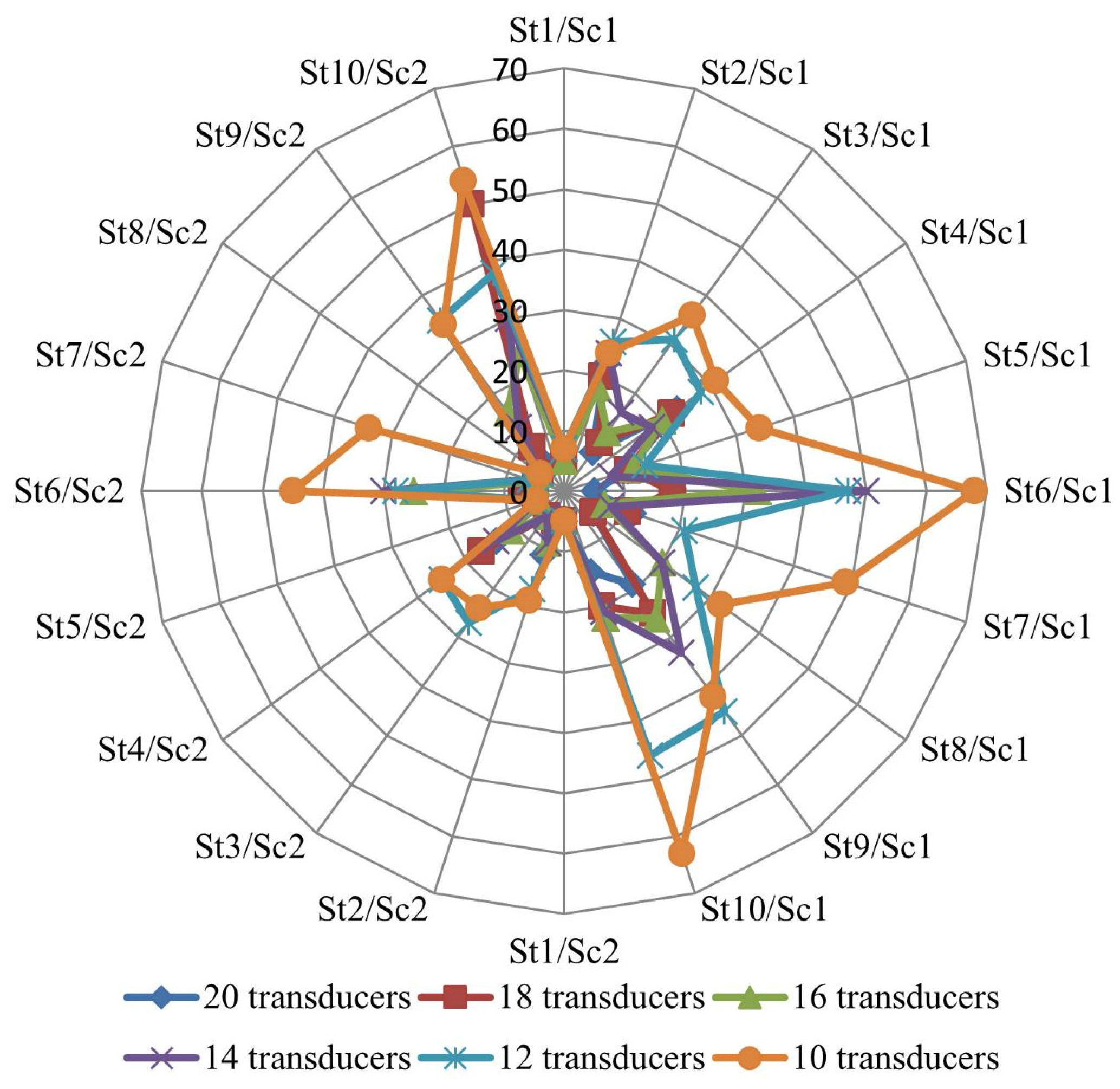
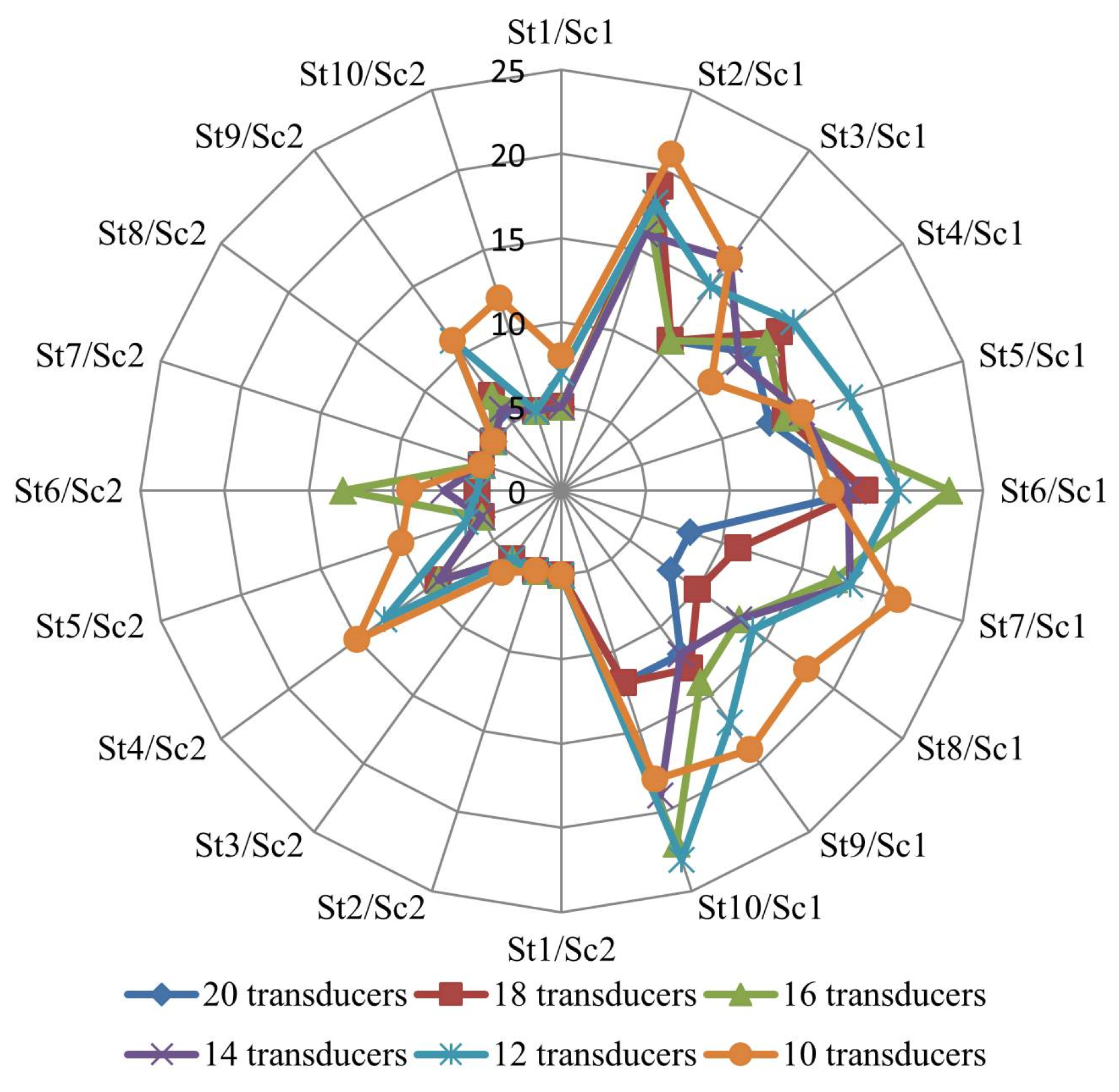
Figure 5 and Figure 6 compare the number of reliable and total leaky pipes, respectively, for ten situations (St1 to St10), with the different sets of pressure transducers, in scenario 1 (right side) and in scenario 2 (left side), for the first WDN.

Figure 5. Number of reliable leaky pipes in the first WDN.

Figure 5. Number of reliable leaky pipes in the first WDN.

Figure 6. Number of total leaky pipes in the first WDN.

Figure 6. Number of total leaky pipes in the first WDN.

For all situations and independently of the number of pressure transducers, the leak flow of each pipe is assigned to the correct pipe or to its adjacent pipes. As a consequence the pipes that might have leaks are circumscribed to a reduced area of the WDN.

The evaluations with fewer pressure transducers tend to spread the leak flow among the correct pipe and its adjacent pipes. Nevertheless, using only ten pressure transducers, there were only two over twenty situations that identified only four out of the five leaky pipes in Table 2. Both occurred in scenario 1, and all other situations identified the leaky pipes correctly. Increasing the number of pressure transducers tends to improve the identification of the leaky pipes and/or the leak flows.

In scenario 2 (bigger leakage flow), the final solutions are globally better than those from scenario 1. The bigger leakage flow is associated with a bigger head loss and the impact in the pressure transducers observations is also bigger. Against the expected, in scenario 2, for situation 4 with 12 monitoring nodes and for situation 10 with 14 monitoring nodes, the searching process stopped prematurely with poor final solutions identifying too many leaky pipes. Nevertheless all leaky pipes were correctly identified in all solutions.

3.3.2. Second WDN

The second water distribution network has a total length of 21.468 km (each pipe presents a half of its original length) and, for the night consumption without leakage, the maximum head loss observed is 0.0196 m. Results from the application of the proposed methodology to both scenarios, with each situation, and assuming different sets of pressure transducers, are summarized in Table 6 and Table 7.

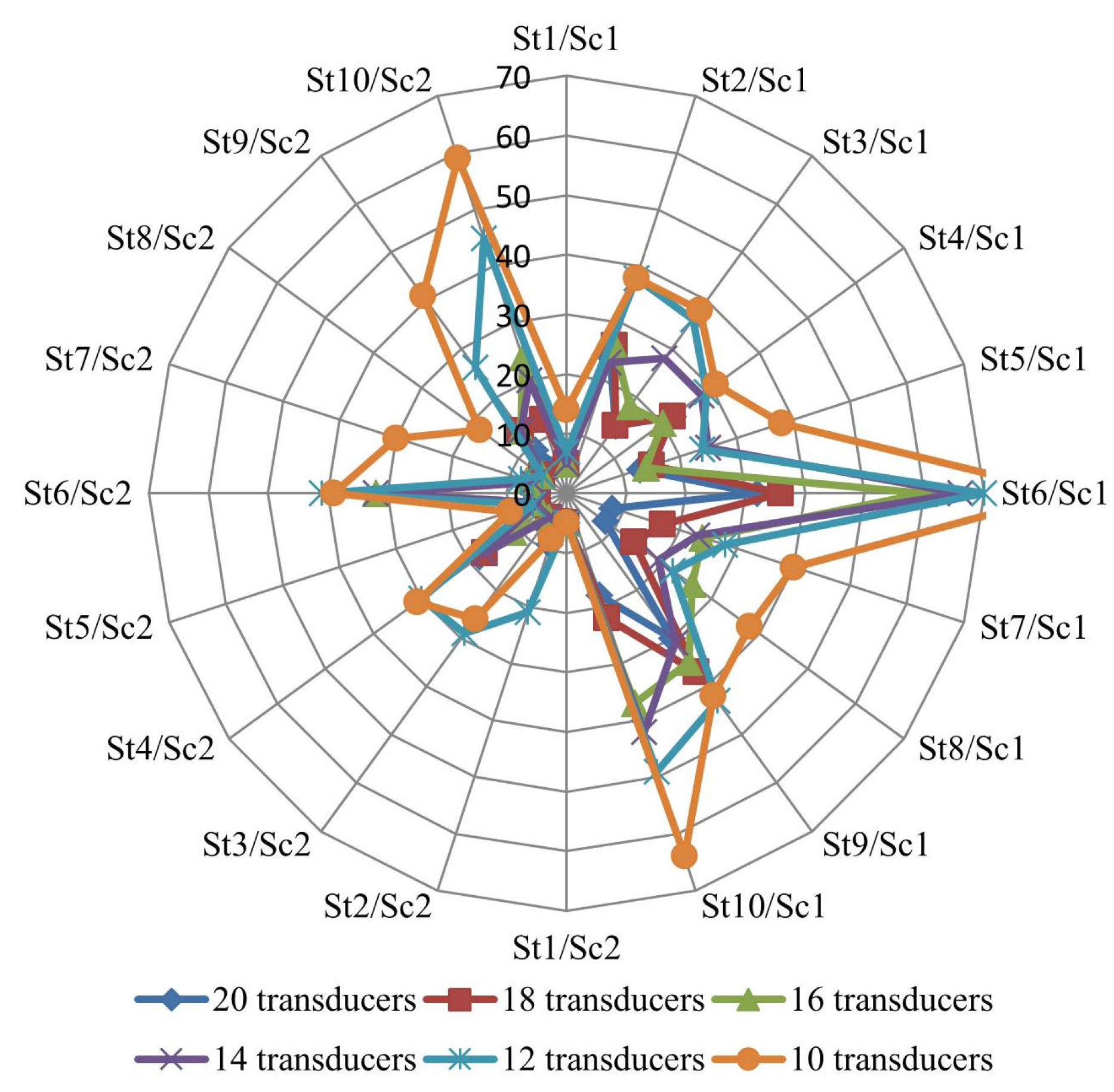
The second WDN has the same consumption and leakage flow of the first WDN, but each pipe has half of the original extension. Consequently, the head loss is also reduced to a half in each correspondent pipe and the pressure transducer observations approach the static pressure value. As previously observed for the first WDN, increasing the number of pressure transducers also yields benefits.

For the second WDN the solutions tend to identify more leaky pipes and the number of reliable pipes increases. Pipes adjacent to the reliable pipes in the first WDN now become reliable pipes. As the number of probable leaky pipes increased, the leakage flow assigned to those pipes decreased.

Figure 7 and Figure 8 compare the number of reliable and total leaky pipes, respectively, for the second WDN.

Table 6. Number of reliable leaky pipes in the second WDN (scenario 1/scenario 2).

Situation	Number of Pressure Transducers
	10	12	14	16	18	20
1	8/5	7/5	5/5	5/5	5/5	5/5
2	21/5	18/5	16/5	17/5	19/5	18/5
3	17/6	15/5	17/5	11/5	11/5	11/5
4	11/15	17/13	13/9	15/9	16/9	14/9
5	15/10	18/6	15/5	14/5	14/5	13/5
6	16/9	20/5	17/7	23/13	18/5	18/5
7	21/5	18/5	18/5	17/5	11/5	8/5
8	18/5	14/5	13/5	13/5	10/5	8/5
9	19/11	17/11	12/6	14/7	13/7	12/6
10	18/12	23/5	19/5	22/5	12/5	12/5

Table 6. Number of reliable leaky pipes in the second WDN (scenario 1/scenario 2).

Situation	Number of Pressure Transducers
	10	12	14	16	18	20
1	8/5	7/5	5/5	5/5	5/5	5/5
2	21/5	18/5	16/5	17/5	19/5	18/5
3	17/6	15/5	17/5	11/5	11/5	11/5
4	11/15	17/13	13/9	15/9	16/9	14/9
5	15/10	18/6	15/5	14/5	14/5	13/5
6	16/9	20/5	17/7	23/13	18/5	18/5
7	21/5	18/5	18/5	17/5	11/5	8/5
8	18/5	14/5	13/5	13/5	10/5	8/5
9	19/11	17/11	12/6	14/7	13/7	12/6
10	18/12	23/5	19/5	22/5	12/5	12/5

Table 7. Number of total leaky pipes in the second WDN (scenario 1/scenario 2).

Situation	Number of Pressure Transducers
	10	12	14	16	18	20
1	14/5	7/5	5/5	5/5	5/5	5/5
2	38/8	38/21	23/5	26/5	26/5	24/9
3	38/26	36/29	28/5	18/5	14/5	14/5
4	31/31	29/30	28/17	20/11	22/17	22/18
5	38/10	24/6	25/5	14/5	15/5	13/5
6	84/39	70/41	66/32	60/32	36/5	32/5
7	40/30	28/8	23/6	24/7	17/5	8/5
8	38/18	22/5	19/5	26/5	14/5	8/5
9	42/41	43/26	31/13	35/13	37/13	30/9
10	64/59	49/45	42/20	37/24	22/13	18/5

Table 7. Number of total leaky pipes in the second WDN (scenario 1/scenario 2).

Situation	Number of Pressure Transducers
	10	12	14	16	18	20
1	14/5	7/5	5/5	5/5	5/5	5/5
2	38/8	38/21	23/5	26/5	26/5	24/9
3	38/26	36/29	28/5	18/5	14/5	14/5
4	31/31	29/30	28/17	20/11	22/17	22/18
5	38/10	24/6	25/5	14/5	15/5	13/5
6	84/39	70/41	66/32	60/32	36/5	32/5
7	40/30	28/8	23/6	24/7	17/5	8/5
8	38/18	22/5	19/5	26/5	14/5	8/5
9	42/41	43/26	31/13	35/13	37/13	30/9
10	64/59	49/45	42/20	37/24	22/13	18/5

Figure 7. Number of reliable leaky pipes in the second WDN.

Figure 7. Number of reliable leaky pipes in the second WDN.

Figure 8. Number of total leaky pipes in the second WDN.

Figure 8. Number of total leaky pipes in the second WDN.

3.4. Discussion of Results

The methodology presented here to locate and quantify leaks is able to identify as many leaky pipes as necessary. It showed its ability to deal with WDN with different characteristics: total length, total leakage flow and leakage flow spatial distribution.

Results confirm that the methodology is effective and robust. In fact, despite the dispersion observed in some of the results, the majority of the pipes with leaks were identified in all the case studies. Solutions from scenario 2 were always better than those from scenario 1, this means, in all situations considered, pipes with greater leakage flows were better identified than the others. It becomes evident that the search procedure tends to get focused on the most problematic pipes (bigger leakage flows) and in those cases the dispersion gets reduced.

The results of the TrustRank algorithm locate the pressure transducers in the periphery, covering the entire WDN.

Concerning the monitoring nodes, results showed that, as expected, more pressure transducers improve the quality of the solutions, reducing the dispersion and increasing the confidence on the identification of the probable leaky pipes and pipes without leakage problems. Results also showed that leaky pipes close to the tank were more difficult to identify and this can be explained by the lower head losses.

In some of the case studies the solutions identified only the correct leaky pipes (mostly for scenario 2 and with more pressure transducers), demonstrating that the methodology can be effective. Additionally, in many other case studies the number of reliable pipes is only slightly higher than the correct number of leaky pipes, which is also a good contribution for the methodology effectiveness. However, in a reduced number of case studies (with fewer pressure transducers) the number of reliable leaky pipes is considerably high showing that the methodology still can be improved. The introduction of more monitoring nodes certainly would contribute to increase the quality of the solutions, but on the other hand it would also increase the cost of acquiring the equipment and gathering data. An alternative is to maintain the number of monitoring nodes and improve their effectiveness by artificially increase the head loss in the WDN [53], but this is a subject to be explored in a future work. A third alternative is to improve the stopping criterion in the simulated annealing algorithm that would continue to search for a longer time.

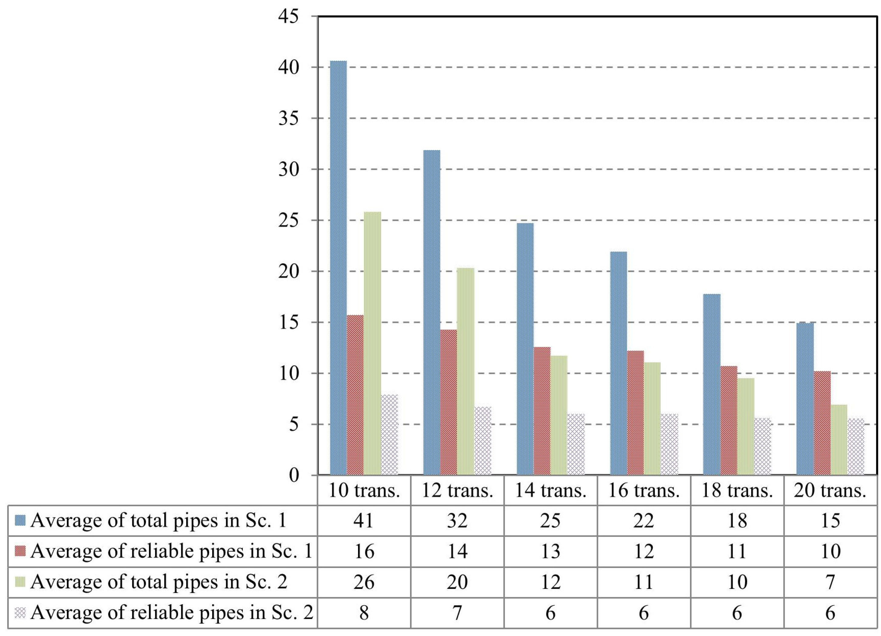
It was observed that the quality of the solutions depends on the total leakage flow and its spatial distribution, the number of monitoring nodes and the position of the leaky pipes in the WDN. Increasing the number of monitoring nodes contributes to improve the quality of the solutions in terms of total leaky pipes identified: the duplication of the monitoring nodes reduces to less than a half the total leaky pipes (Figure 9 and Figure 10). But the total leakage flow also plays an important role: the number of total leaky pipes is reduced to about a half with a ten times increase in the total leakage flow (scenarios 1 and 2), eliminating most of the false leaky pipes (Figure 9).

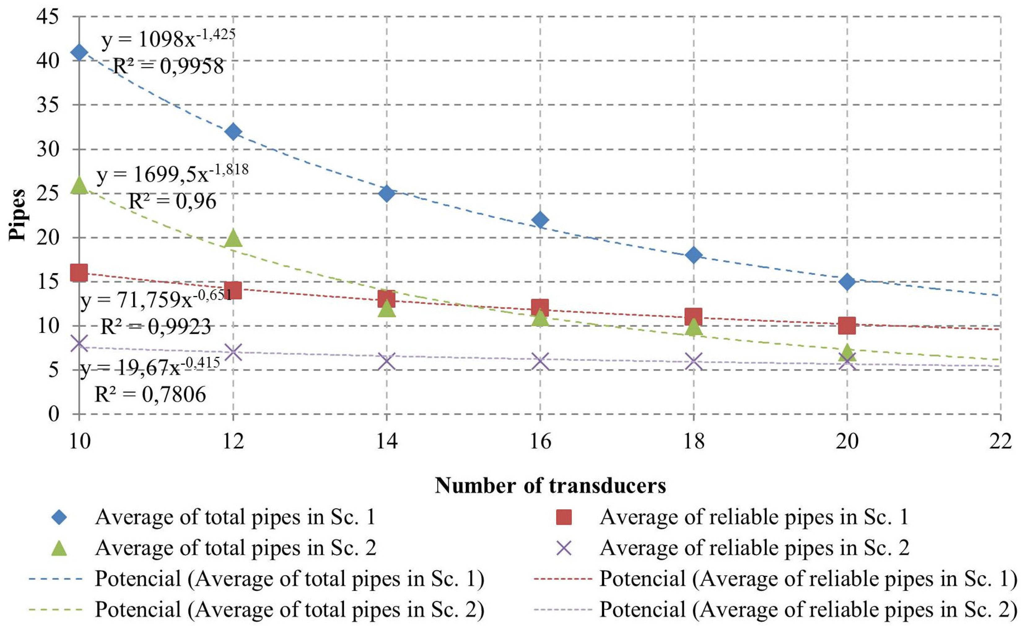
Figure 10 presents a relationship between the number of transducers and the average number of potential leaky pipes identified. As expected, when the number of pressure transducers increases, the number of potential leaky pipes decreases, which means that the pipes identified have a high probability of being leaky. The presence of additional pressure transducers decreases mainly the average number of total pipes for both scenarios, and it can be seen that the improvement obtained follows a power law.

Figure 9. Average of total and reliable leaky pipes for both scenarios and the two WDN.

Figure 9. Average of total and reliable leaky pipes for both scenarios and the two WDN.

Figure 10. Relationship between the number of pressure transducers and the number of total and reliable pipes.

Figure 10. Relationship between the number of pressure transducers and the number of total and reliable pipes.

4. Conclusions

Minimize water loss is an important task for any water company. This paper presented a methodology that uses a hydraulic model of the WDN to quickly and economically identify probable leaky pipes. This methodology is based on pressure measurements and explores the exchange of information between an optimization model and the hydraulic simulation of the WDN in steady state conditions. The pressure transducer placement is carried out by a novel tool based on the TrustRank algorithm, specifically developed to select the monitoring nodes, demonstrating ability to gather the necessary information for the methodology to work. The optimization model used to identify the leaky pipes is solved by a simulated annealing algorithm, a reliable, fast, and easy to implement method.

The results obtained for a set of 240 case studies (two networks, two leakage flow scenarios, ten spatial distributions of the leakage flow and six sets of pressure transducers) are very encouraging. The implementation of the methodology does not affect the regular activity of the WDN and it is able to identify existing leaky pipes. Results showed that, in general, this leak location procedure identifies a small number of pipes, confining the inspection works to a considerably reduced extension of the WDN.

Future works include the analysis of the WDN in quasi-steady state conditions and apply it to a real WDN to confirm its effectiveness.

References

- Henry, M. Water: Facts without Myths. Water 2009, 1, 3–4. [Google Scholar] [CrossRef]
- Wu, Z.; Song, Y. Optimizing pressure logger placement for leakage detection and model calibration. In WDSA 2012; Engineers Australia: Adelaide, Australia, 2012. [Google Scholar]
- Vítkovský, J.P.; Liggett, J.; Simpson, A.; Lambert, M.F. Optimal measurement site locations for inverse transient analysis in pipe networks. J. Water Resour. Plan. Manag. 2003, 129, 480–492. [Google Scholar] [CrossRef]
- Kang, D.; Lansey, K. Optimal meter placement for water distribution system state estimation. J. Water Resour. Plan. Manag. 2010, 136, 337–348. [Google Scholar] [CrossRef]
- Goulet, J.; Coutu, S.; Smith, I.F.C. Model falsification diagnosis and sensor placement for leak detection in pressurized pipe networks. Adv. Eng. Inform. 2013, 27, 261–269. [Google Scholar] [CrossRef]
- Pilcher, R. Leak detection practices and techniques: A practical approach. Water21, December 2003; 44–45. [Google Scholar]
- Lambert, A. Assessing non-revenue water and its components: A practical approach. Water21, August 2003; 50–51. [Google Scholar]
- Farley, B.; Mounce, S.R.; Boxall, J.B. Field testing of an optimal sensor placement methodology for event detection in an urban water distribution network. Urban Water J. 2010, 7, 345–356. [Google Scholar] [CrossRef]
- Candelieri, A.; Soldi, D.; Conti, D.; Archetti, F. Analytical leakages localization in water distribution networks through spectral clustering and support vector machines. The icewater approach. Procedia Eng. 2014, 89, 1080–1088. [Google Scholar] [CrossRef]
- Bort, C.M.G.; Righetti, M.; Bertola, P. Methodology for leakage isolation using pressure sensitivity and correlation analysis in water distribution systems. Procedia Eng. 2014, 89, 1561–1568. [Google Scholar] [CrossRef]
- Blesa, J.; Nejjari, F.; Sarrate, R. Robustness analysis of sensor placement for leak detection and location under uncertain operating conditions. Procedia Eng. 2014, 89, 1553–1560. [Google Scholar] [CrossRef] [Green Version]
- Steffelbauer, D.; Neumayer, M.; Gunther, M.; Fuchs-Hanusch, D. Sensor placement and leakage localization considering demand uncertainties. Procedia Eng. 2014, 89, 1160–1167. [Google Scholar] [CrossRef]
- Gabrys, B.; Bargiela, A. Analysis of uncertainties in water systems using neural networks. Measur. Control 1999, 32, 145–147. [Google Scholar] [CrossRef]
- Gabrys, B.; Bargiela, A. Neural networks based decision support in presence of uncertainties. J. Water Resour. Plan. Manag. 1999, 125, 272–280. [Google Scholar] [CrossRef]
- Mounce, S.; Machell, J. Burst detection using hydraulic data from water distribution systems with artificial neural networks. Urban Water J. 2006, 3, 21–31. [Google Scholar] [CrossRef]
- Caputo, A.C.; Pelagagge, P.M. An inverse approach for piping networks monitoring. J. Loss Prev. Process Ind. 2002, 15, 497–505. [Google Scholar] [CrossRef]
- Poulakis, Z.; Valougeorgis, D.; Papadimitriou, C. Leakage detection in water pipe networks using a Bayesian probabilistic framework. Probab. Eng. Mech. 2003, 18, 315–327. [Google Scholar] [CrossRef]
- Qi, S.; Wu, W.; Qiao, Y.; Tu, M.; Wang, J. Research on an optimized leakage locating model in water distribution system. Procedia Eng. 2014, 89, 1569–1576. [Google Scholar] [CrossRef]
- Mounce, S.R.; Boxall, J.B.; Machell, J. Online Application of ANN and Fuzzy Logic System for burst detection. In Proceedings of the 10th International Water Distribution System Analysis Conference, Kruger National Park, South Africa, 17–20 August 2008; Van Zyl, J.E., Ilemobade, A.A., Jacobs, H.E., Eds.; pp. 735–746.
- Islam, M.S.; Sadiq, R.; Rodriguez, M.; Francisque, A.; Najjaran, H.; Hoorfar, M. Leakage detection and location in water distribution systems using a fuzzy-based methodology. Urban Water J. 2011, 8, 351–365. [Google Scholar] [CrossRef]
- Aksela, K.; Aksela, M.; Vahala, R. Leakage detection in a real distribution network using a SOM. Urban Water J. 2009, 6, 279–289. [Google Scholar] [CrossRef]
- Gertler, J.; Romera, J.; Puig, V.; Quevedo, J. Leak detection and isolation in water distribution networks using principal component analysis and structured residuals. In Proceedings of the 2010 Conference on Control and Fault-Tolerant Systems (SysTol), Nice, France, 6–8 October 2010; pp. 191–196.
- Jung, D.; Lansey, K. Water distribution system burst detection using a nonlinear kalman filter. J. Water Resour. Plan. Manag. 2014. [Google Scholar] [CrossRef]
- Okeya, I.; Kapelan, Z.; Hutton, C.; Naga, D. Online burst detection in a water distribution system using the kalman filter and hydraulic modelling. Procedia Eng. 2014, 89, 418–427. [Google Scholar] [CrossRef] [Green Version]
- Kang, D.; Lansey, K. Novel approach to detecting pipe bursts in water distribution networks. J. Water Resour. Plan. Manag. 2014, 140, 121–127. [Google Scholar] [CrossRef]
- Ormsbee, L.E. Implicit Network Calibration. J. Water Resour. Plan. Manag. 1989, 115, 243–257. [Google Scholar] [CrossRef]
- Pudar, R.; Liggett, J. Leaks in pipe networks. J. Hydraul. Eng. 1992, 118, 1031–1046. [Google Scholar] [CrossRef]
- Andersen, J.H.; Powell, R.S. Implicit state-estimation technique for water network monitoring. Urban Water 2000, 2, 123–130. [Google Scholar] [CrossRef]
- Puust, R.; Kapelan, Z.; Savic, D.; Koppel, T. Probabilistic Leak Detection in Pipe Networks Using the SCEM-UA Algorithm. In Proceedings of the Water Distribution Systems Analysis Symposium, Cincinnati, OH, USA, 27–30 August 2006; American Society of Civil Engineers: Reston, VA, USA, 2006; Volume 40941, pp. 1–12. [Google Scholar]
- Liggett, J.; Chen, L. Inverse transient analysis in pipe networks. J. Hydraul. Eng. 1994, 120, 934–955. [Google Scholar] [CrossRef]
- Colombo, A.F.; Lee, P.; Karney, B.W. A selective literature review of transient-based leak detection methods. J. Hydro-Environ. Res. 2009, 2, 212–227. [Google Scholar] [CrossRef]
- Puust, R.; Kapelan, Z.; Savic, D.; Koppel, T. A review of methods for leakage management in pipe networks. Urban Water J. 2010, 7, 25–45. [Google Scholar] [CrossRef]
- Lay-Ekuakille, A.; Vendramin, G.; Trotta, A. Robust spectral leak detection of complex pipelines using filter diagonalization method. IEEE Sens. J. 2009, 9, 1605–1614. [Google Scholar] [CrossRef]
- Lay-Ekuakille, A.; Griffo, G.; Vergallo, P. Robust algorithm based on decimated Padè approximant technique for processing sensor data in leak detection in waterworks. IET Sci. Measur. Technol. 2013, 7, 256–264. [Google Scholar] [CrossRef]
- Kim, S. Inverse transient analysis for a branched pipeline system with leakage and blockage using impedance method. Procedia Eng. 2014, 89, 1350–1357. [Google Scholar] [CrossRef]
- Ferrante, M.; Brunone, B.; Meniconi, S. Wavelets for the analysis of transient pressure signals for leak detection. J. Hydraul. Eng. 2007, 133, 1274–1282. [Google Scholar] [CrossRef]
- Ferrante, M.; Brunone, B.; Meniconi, S. Leak-edge detection. J. Hydraul. Res. 2009, 47, 233–241. [Google Scholar] [CrossRef]
- Brunone, B.; Ferrante, M.; Meniconi, S. Portable pressure wave-maker for leak detection and pipe system characterization. J. Am. Water Work. Assoc. 2008, 100, 108–116. [Google Scholar]
- Ferrante, M.; Brunone, B.; Meniconi, S. Leak detection in branched pipe systems coupling wavelet analysis and a Lagrangian model. J. Water Supply Res. Technol. 2009, 58, 95–106. [Google Scholar] [CrossRef]
- Meniconi, S.; Brunone, B.; Asce, M.; Ferrante, M.; Massari, C. Potential of transient tests to diagnose real supply pipe systems: What can be done with a single extemporary test. J. Water Resour. Plan. Manag. 2011, 137, 238–241. [Google Scholar] [CrossRef]
- Izquierdo, J.; Montalvo, I.; Pérez, R.; Tavera, M. Optimization in water systems: A PSO approach. In Proceedings of the Business and Industry Symposium, Ottawa, ON, Canada, 14–17 April 2008; pp. 239–246.
- Almandoz, J.; Cabrera, E.; Arregui, F.; Cabrera, E., Jr.; Cobacho, R. Leakage assessment through water distribution network simulation. J. Water Resour. Plan. Manag. 2005, 131, 458–466. [Google Scholar] [CrossRef]
- Pérez, R.; Sanz, G.; Puig, V.; Quevedo, J.; Ângel, M.; Escofet, C.; Nejjari, F.; Meseguer, J.; Cembrano, G.; Tur, J.; Sarrate, R. Leak localization in water networks—A model-based methodology using pressure sensors applied to a real network in Barcelona. IEEE 2014, 24–36. [Google Scholar]
- Giustolisi, O.; Savic, D.; Kapelan, Z. Pressure-driven demand and leakage simulation for water distribution networks. J. Hydraul. Eng. 2008, 134, 626–635. [Google Scholar] [CrossRef]
- Muranho, J.; Ferreira, A.; Sousa, J.; Gomes, A.; Sá-Marques, A. Pressure-dependent demand and leakage modelling with an EPANET extension—WaterNetGen. Procedia Eng. 2014, 89, 632–639. [Google Scholar] [CrossRef]
- Wu, Z.; Sage, P. Water loss detection via genetic algorithm optimization-based model calibration. In Proceedings of the ASCE 8th Annual International Synposium on Water Distribution System Analysis, Cincinnati, OH, USA, 27–30 Agust 2006; pp. 1–11.
- Wu, Z.; Sage, P.; Turtle, D. Pressure-dependent leak detection model and its application to a district water system. J. Water Resour. Plan. Manag. 2010, 136, 116–128. [Google Scholar] [CrossRef]
- Ribeiro, L.; Muranho, J.; Sousa, J.; Sá-Marques, A. Identificação de fugas através de modelação matemática de redes de distribuição de água. In 15° ENaSB—Encontro de Engenharia Sanitária e Ambiental; Reorganização para a Sustentabilidade do Setor das Águas e Resíduos; APESB: Évora, Portugal, 2012. (In Portuguese) [Google Scholar]
- Sousa, J. Decision Aid Models for the Design and the Operation of Water Supply Systems. Ph.D. Thesis, Coimbra University, Coimbra, Portugal, 2006. [Google Scholar]
- Vítkovský, B.J.P.; Simpson, A.R.; Lambert, M.F. Leak detection and calibration using transients and genetic algorithms. J. Water Resour. Plan. Manag. 2000, 126, 262–265. [Google Scholar] [CrossRef]
- Izquierdo, J.; Pérez, R.; Iglesias, P.L. Mathematical models and methods in the water industry. Math. Comput. Model. 2004, 39, 1353–1374. [Google Scholar] [CrossRef]
- Mays, L.W. Water Distribution Systems Handbook; American Water Works Association, Ed.; McGraw-Hill: New York, NY, USA, 1999. [Google Scholar]
- Ribeiro, L.; Sousa, J.; Sá Marques, A. Improving the efficiency of leak location via optimal pressure sensor placement in water distribution networks. Water Util. J. 2012, 4, 3–12. [Google Scholar]
- Machell, J.; Mounce, S.R.; Boxall, J.B. Online modelling of water distribution systems: A UK case study. Drink. Water Eng. Sci. 2010, 3, 21–27. [Google Scholar] [CrossRef]
- Costa, A.L.H.; de Medeiros, J.L.; Pessoa, F.L.P. Optimization of pipe networks including pumps by simulated annealing. Braz. J. Chem. Eng. 2000, 17, 887–895. [Google Scholar] [CrossRef]
- Walski, B.T.M. Technique for calibrating network models. J. Water Resour. Plan. Manag. 1984, 109, 360–372. [Google Scholar] [CrossRef]
- Kirkpatrick, S.; Gelatt, C.D.; Vecchi, M.P. Optimization by simulated annealing. Science 1983, 220, 671–680. [Google Scholar] [CrossRef] [PubMed]
- Kirkpatrick, S. Optimization by simulated annealing: Quantitative studies. J. Stat. Phys. 1984, 34, 975–986. [Google Scholar] [CrossRef]
- Kalai, A.T.; Vempala, S. Simulated annealing for convex optimization. Math. Oper. Res. 2006, 31, 253–266. [Google Scholar] [CrossRef]
- Cunha, M.C.; Sousa, J. Water distribution network design optimization: simulated annealing approach. J. Water Resour. Plan. Manag. 1999, 125, 215–221. [Google Scholar] [CrossRef]
- Cunha, M.C.; Sousa, J. Robust design of water distribution networks for a proactive risk management. J. Water Resour. Plan. Manag. 2010, 136, 227–236. [Google Scholar] [CrossRef]
- Marques, J.; Cunha, M.C.; Sousa, J.; Savic, D. Robust optimization methodologies for water supply systems design. Drink. Water Eng. Sci. 2012, 5, 31–37. [Google Scholar] [CrossRef] [Green Version]
- Goldman, F.E.; Mays, L.W. Water distribution system operation: Application of simulated annealing. In Water Resouces Systems Management Tools; Mays, L.W., Ed.; McGraw-Hill: New York, NY, USA, 2005; pp. 5.1–5.17. [Google Scholar]
- Sousa, J.; Cunha, M.C.; Sá-Marques, A. Simulated annealing reaches “ANYTOWN”. In Proceedings of the 8th International Conference on Computing and Control in the Water Industry—CCWI, Exeter, UK, 5–7 September 2005; pp. 69–74.
- Gomes, R.; Sá Marques, A.; Sousa, J. Estimation of the benefits yielded by pressure management in water distribution systems. Urban Water J. 2011, 8, 65–77. [Google Scholar] [CrossRef]
- Gomes, R.; Sá Marques, A.; Sousa, J. District metered areas design under different decision makers’ options: Cost analysis. Water Resour. Manag. 2013, 27, 4527–4543. [Google Scholar] [CrossRef]
- Teegavarapu, R.S.V.; Simonovic, S.P. Optimal Operation of reservoir systems using Simulated Annealing. Water Resour. Manag. 2002, 16, 401–428. [Google Scholar] [CrossRef]
- Khodabakhshi, F.; Ghirian, A.R.; Khakzad, N. Applying simulated annealing for optimal operation of multi-reservoir systems. Am. J. Eng. Appl. Sci. 2009, 1, 80–87. [Google Scholar]
- Locatelli, M. Convergence of a simulated annealing algorithm for continuous global optimization. J. Glob. Optim. 2000, 18, 219–234. [Google Scholar] [CrossRef]
- Gyöngyi, Z.; Garcia-Molina, H.; Pedersen, J. Combating Web Spam with Trustrank. In Proceedings of the Thirtieth International Conference on Very Large Data Bases (VLDB), Toronto, ON, Canada, 31 August–3 September 2004; Morgan Kaufmann: Toronto, ON, Canada, 2004; pp. 576–587. [Google Scholar]
- Yazdani, A.; Jeffrey, P. Complex network analysis of water distribution systems. Chaos 2011, 21, 016111. [Google Scholar] [CrossRef] [PubMed]
© 2015 by the authors; licensee MDPI, Basel, Switzerland. This article is an open access article distributed under the terms and conditions of the Creative Commons Attribution license (http://creativecommons.org/licenses/by/4.0/).
Share and Cite
MDPI and ACS Style
Ribeiro, L.; Sousa, J.; Marques, A.S.; Simões, N.E. Locating Leaks with TrustRank Algorithm Support. Water 2015, 7, 1378-1401. https://doi.org/10.3390/w7041378
AMA Style
Ribeiro L, Sousa J, Marques AS, Simões NE. Locating Leaks with TrustRank Algorithm Support. Water. 2015; 7(4):1378-1401. https://doi.org/10.3390/w7041378
Chicago/Turabian StyleRibeiro, Luísa, Joaquim Sousa, Alfeu Sá Marques, and Nuno E. Simões. 2015. "Locating Leaks with TrustRank Algorithm Support" Water 7, no. 4: 1378-1401. https://doi.org/10.3390/w7041378