
Extending the Global Sensitivity Analysis of the SimSphere model in the Context of its Future Exploitation by the Scientific Community

 ,
, 

Abstract
:1. Introduction

| Previously Examined Model Outputs | New Model Outputs Examined |
|---|---|
| Daily Average Net Radiation () | Daily Average Longwave Downwelling Radiation () |
| Daily Average Tair at 50m () | Daily Average Longwave Upwelling Radiation () |
| Daily Average Evaporative Fraction () | - |
| Daily Average Non-Evaporative Fraction () | - |
| Daily Average Latent Heat flux () | - |
| Daily Average Sensible Heat flux () | - |
| Daily Average Radiometric Temperature () | - |
| Daily Average Surface Soil Moisture Availability | - |
| Daily Average Shortwave Incoming Radiation () | - |
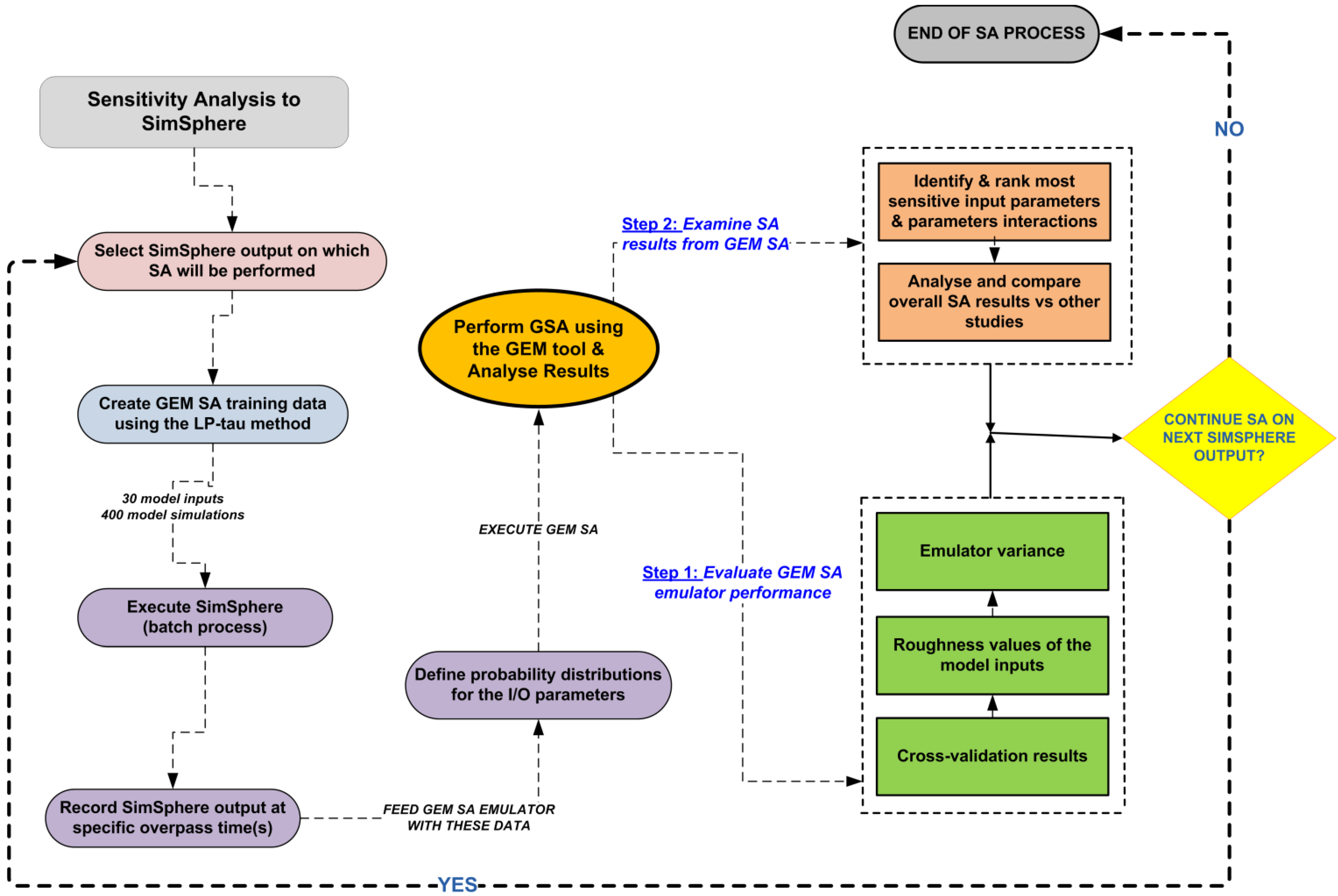
2. Materials and Methods
2.1. SimSphere Land Biosphere Model
2.2. BACCO GSA: Principles
2.3. GSA BACCO Implementation on SimSphere

| Model Input Short Name | Actual Name of the Model Input | Process in which each Parameter is Involved | Min Value | Max Value | |
|---|---|---|---|---|---|
| X1 | Slope (°) | time & location | 0 | 45 | |
| X2 | Aspect (degrees) | time & location | 0 | 360 | |
| X3 | Station Height (m) | time & location | 0 | 4.92 | |
| X4 | Fractional Vegetation Cover (%) | vegetation | 0 | 100 | |
| X5 | LAI (m2·m−2) | vegetation | 0 | 10 | |
| X6 | Foliage emissivity (unitless) | vegetation | 0.951 | 0.990 | |
| X7 | [Ca] (external CO2 on the leaf) (ppmv) | vegetation | 250 | 710 | |
| X8 | [Ci] (internal CO2 in the leaf) (ppmv) | vegetation | 110 | 400 | |
| X9 | [03] (ozone concentration in the air) (ppmv) | vegetation | 0.0 | 0.25 | |
| X10 | Vegetation height (m) | vegetation | 0.021 | 20.0 | |
| X11 | Leaf width (m) | vegetation | 0.012 | 1.0 | |
| X12 | Minimum Stomatal Resistance (s·m−1) | plant | 10 | 500 | |
| X13 | Cuticle Resistance (s·m−1) | plant | 200 | 2000 | |
| X14 | Critical leaf water potential (bar) | plant | −30 | −5 | |
| X15 | Critical solar parameter (W·m−2) | plant | 25 | 300 | |
| X16 | Stem resistance (s·m−1) | plant | 0.011 | 0.150 | |
| X17 | Surface Moisture Availability (vol/vol) | hydrological | 0 | 1 | |
| X18 | Root Zone Moisture Availability (vol/vol) | hydrological | 0 | 1 | |
| X19 | Substrate Max. Volum. Water Content (vol/vol) | hydrological | 0.01 | 1 | |
| X20 | Substrate climatol. mean temperature (°C) | surface | 20 | 30 | |
| X21 | Thermal inertia (W·m−2·K−1) | surface | 3.5 | 30 | |
| X22 | Ground emissivity (unitless) | surface | 0.951 | 0.980 | |
| X23 | Atmospheric Precipitable water (cm) | meteorological | 0.05 | 5 | |
| X24 | Surface roughness (m) | meteorological | 0.02 | 2.0 | |
| X25 | Obstacle height (m) | meteorological | 0.02 | 2.0 | |
| X26 | Fractional Cloud Cover (%) | meteorological | 1 | 10 | |
| X27 | RKS (satur. thermal conduct.(Cosby et al., [76]) | soil | 0 | 10 | |
| X28 | Cosby B (see Cosby et al., [76]) | soil | 2.0 | 12.0 | |
| X29 | THM (satur.vol. water cont.) (Cosby et al., [76]) | soil | 0.3 | 0.5 | |
| X30 | PSI (satur. water potential) (Cosby et al., [76]) | soil | 1 | 7 | |
3. Results
3.1. Emulator Accuracy
| Emulator Statistics | 07:30 | 09:30 | 11:30 | 13:30 | 15:30 | 17:00 | 07:30 | 09:30 | 11:30 | 13:30 | 15:30 | 17:00 |
|---|---|---|---|---|---|---|---|---|---|---|---|---|
| Sigma-squared | 1.204 | 1.192 | 1.619 | 1.588 | 1.746 | 1.235 | 1.274 | 1.160 | 1.661 | 1.766 | 1.298 | 1.443 |
| Cross- validation root mean squared-error: | 14.150 | 30.396 | 34.776 | 36.468 | 31.922 | 24.003 | 1.859 | 1.729 | 2.080 | 2.693 | 2.837 | 4.653 |
| Cross-validation root mean squared relative error (%): | 63.275 | 46.927 | 41.633 | 39.840 | 57.685 | 3.8E+16 | 0.635 | 0.586 | 0.693 | 0.888 | 0.924 | 1.485 |
| Cross-validation root mean squared standardised error: | 1.229 | 1.817 | 1.790 | 1.581 | 1.471 | 1.439 | 1.090 | 1.210 | 1.543 | 1.519 | 1.452 | 1.749 |
| Sigma-squared | 1.054 | 1.294 | 1.483 | 1.640 | 1.750 | 1.481 | 0.571 | 0.461 | 0.533 | 0.689 | 1.101 | 1.299 |
| Cross- validation root mean squared-error: | 0.079 | 0.097 | 0.082 | 0.083 | 0.086 | 0.103 | 6.490 | 8.277 | 13.611 | 16.939 | 25.004 | 21.593 |
| Cross-validation root mean squared relative error (%): | 23.668 | 26.805 | 25.292 | 30.599 | 34.329 | 1.5E+17 | 1.597 | 1.837 | 2.701 | 3.222 | 4.523 | 4.208 |
| Cross-validation root mean squared standardised error: | 1.364 | 1.667 | 1.717 | 1.527 | 1.274 | 1.402 | 1.313 | 0.926 | 1.151 | 1.121 | 1.562 | 1.432 |
| Sigma-squared | 1.149 | 0.676 | 1.057 | 1.198 | 1.428 | 1.395 | 0.234 | 0.174 | 0.161 | 0.181 | 0.269 | 0.242 |
| Cross- validation root mean squared-error: | 13.764 | 18.554 | 28.798 | 28.644 | 43.513 | 32.586 | 9.685 | 15.273 | 13.705 | 13.903 | 13.18 | 19.601 |
| Cross-validation root mean squared relative error (%): | 50.82 | 21.214 | 23.485 | 21.000 | 48.819 | 54.113 | 3.543 | 5.322 | 2.543 | 2.383 | 2.453 | 8.507 |
| Cross-validation root mean squared standardised error: | 1.227 | 1.490 | 1.484 | 1.197 | 1.522 | 1.262 | 0.654 | 0.889 | 0.928 | 0.895 | 0.673 | 0.885 |
| Sigma-squared | 1.054 | 1.294 | 1.483 | 1.64 | 1.750 | 1.490 | 0.335 | 0.280 | 0.413 | 0.486 | 0.788 | 0.507 |
| Cross- validation root mean squared-error: | 0.079 | 0.097 | 0.082 | 0.083 | 0.086 | 0.106 | 15.641 | 21.130 | 25.060 | 29.998 | 38.739 | 28.731 |
| Cross-validation root mean squared relative error (%): | 22.624 | 29.190 | 20.033 | 19.513 | 33.786 | 60.542 | 8.988 | 8.982 | 6.349 | 7.495 | 13.288 | 115.665 |
| Cross-validation root mean squared standardised error: | 1.364 | 1.667 | 1.717 | 1.527 | 1.274 | 1.462 | 1.343 | 1.212 | 1.111 | 1.212 | 1.234 | 1.332 |
| Sigma-squared | - | 0.088 | 1.240 | 0.181 | 0.216 | 0.209 | 1.142 | 1.475 | 1.630 | 1.642 | 1.281 | 1.438 |
| Cross- validation root mean squared-error: | - | 33.152 | 31.012 | 48.942 | 38.941 | 43.343 | 0.271 | 0.361 | 0.491 | 0.633 | 0.688 | 1.004 |
| Cross-validation root mean squared relative error (%): | - | 30.294 | 19.814 | 74.858 | 22.661 | 74.416 | 1.931 | 2.411 | 3.030 | 3.749 | 3.928 | 5.336 |
| Cross-validation root mean squared standardised error: | - | 1.555 | 1.474 | 1.429 | 1.490 | 1.367 | 1.277 | 1.273 | 1.505 | 1.510 | 1.471 | 1.932 |
| Sigma-squared | 0.690 | 0.695 | 0.875 | 1.146 | 1.801 | 1.444 | ||||||
| Cross- validation root mean squared-error: | 1.774 | 2.549 | 2.771 | 4.074 | 4.506 | 4.488 | ||||||
| Cross-validation root mean squared relative error (%): | 7.705 | 8.733 | 7.913 | 10.724 | 11.322 | 12.185 | ||||||
| Cross-validation root mean squared standardised error: | 1.355 | 1.368 | 1.117 | 1.575 | 1.121 | 1.318 | ||||||
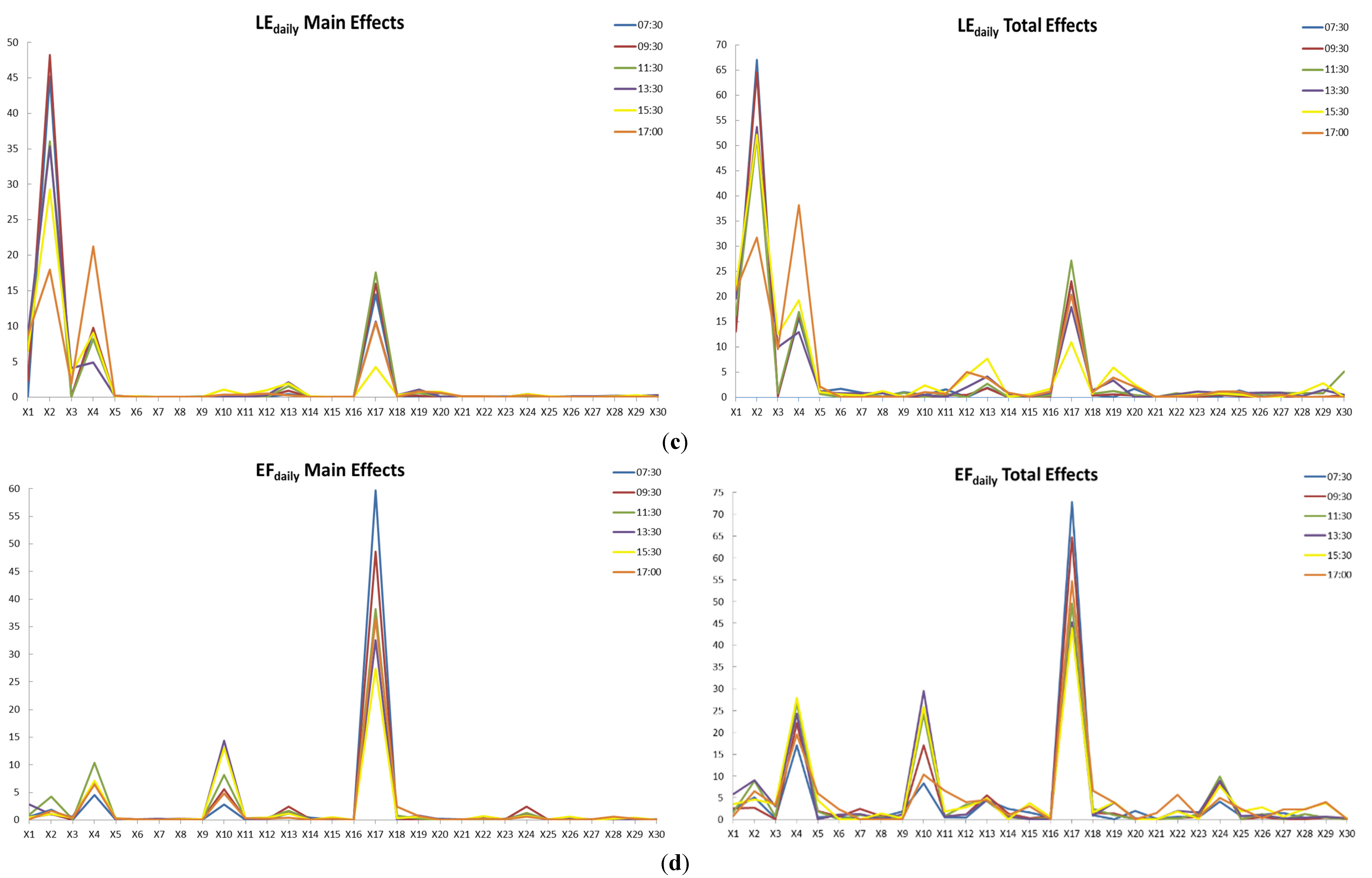
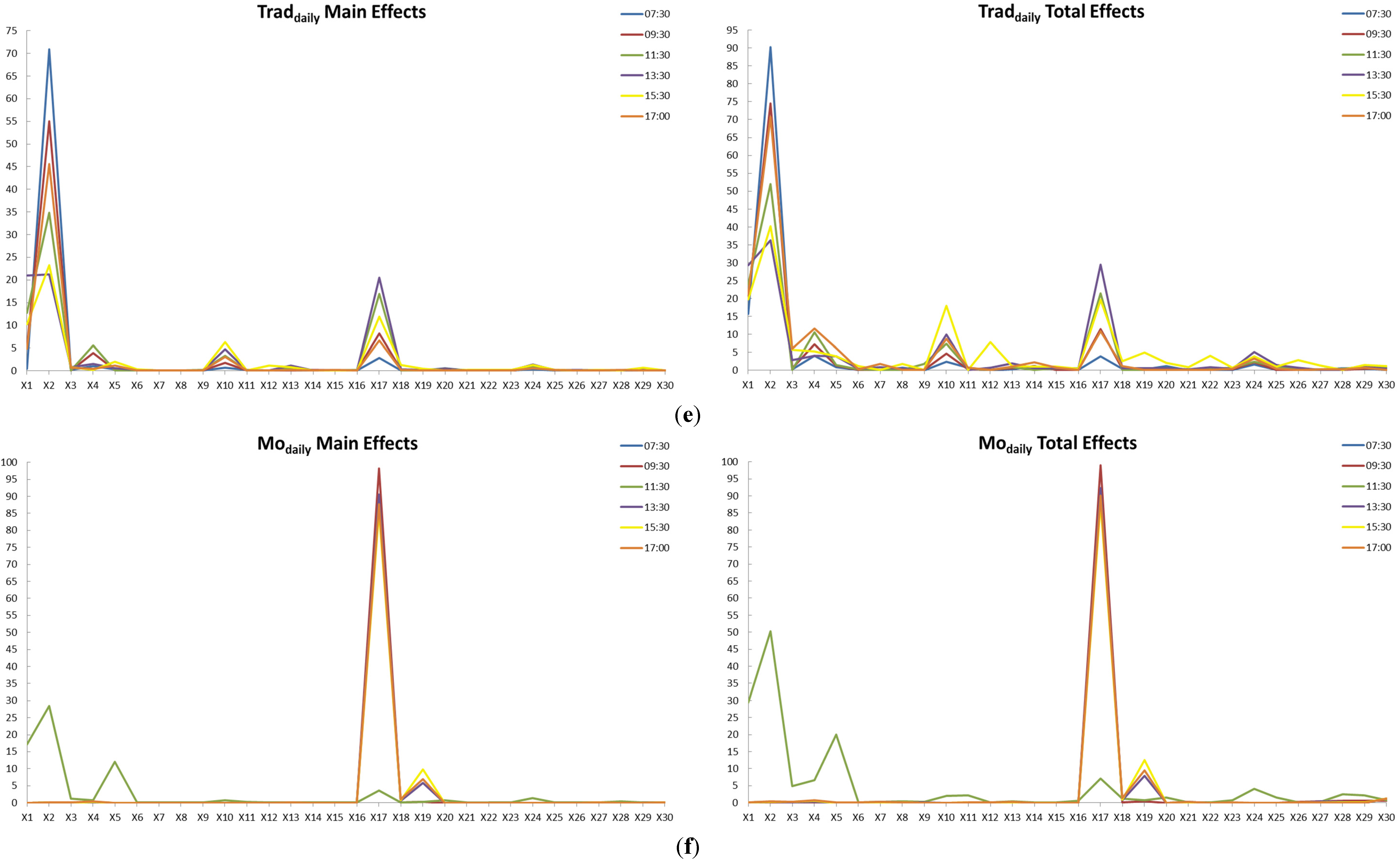
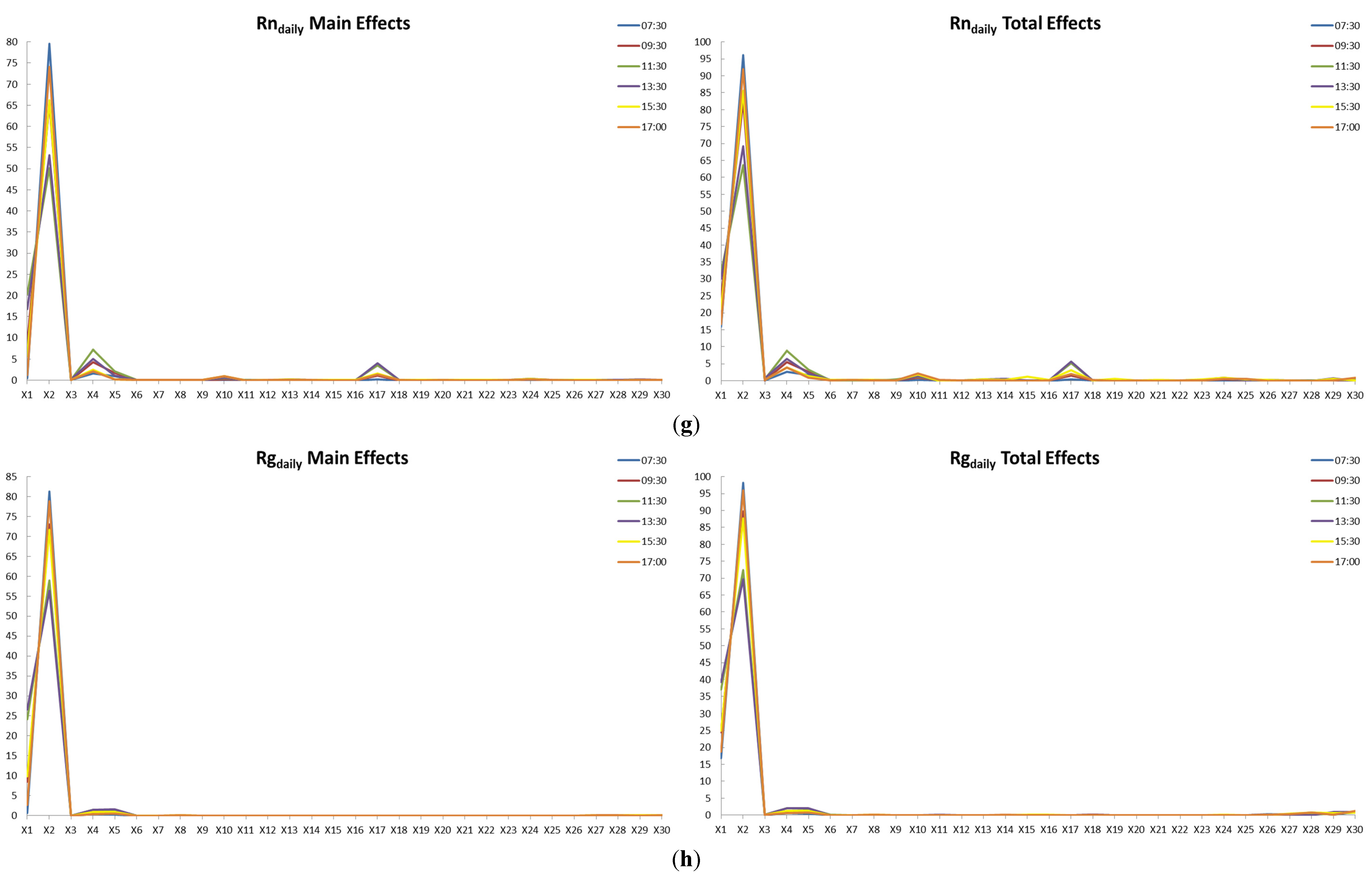
3.2. SA Results
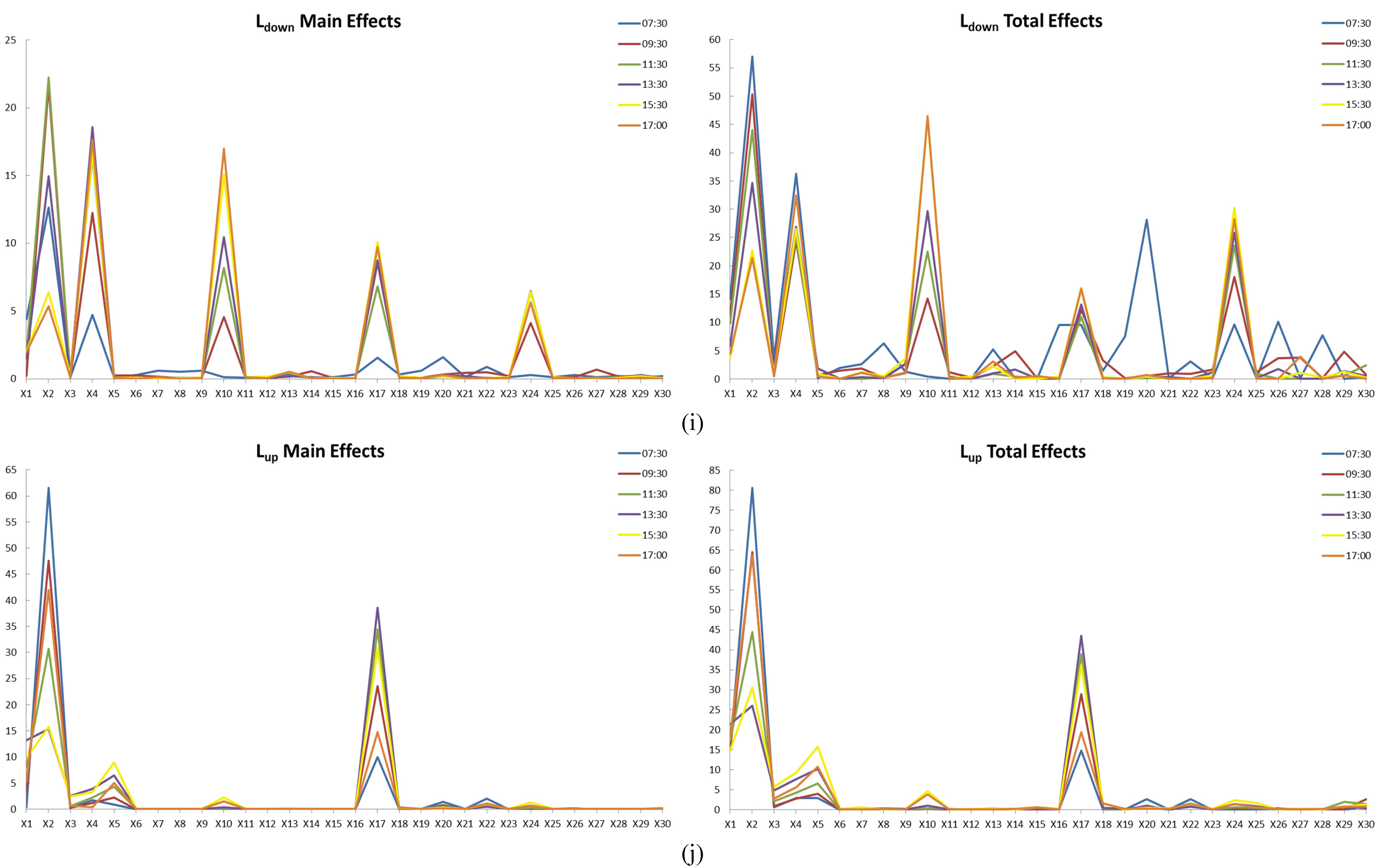
3.2.1. Parameter Sensitivity for ()
3.2.2. Parameter Sensitivity for ()
3.2.3. Parameter Sensitivity for ()
3.2.4. Parameter Sensitivity for ()
3.2.5. Parameter Sensitivity for () and ()
3.2.6. Parameter Sensitivity for ()
3.2.7. Parameter Sensitivity for ()
3.2.8. Parameter Sensitivity for ()
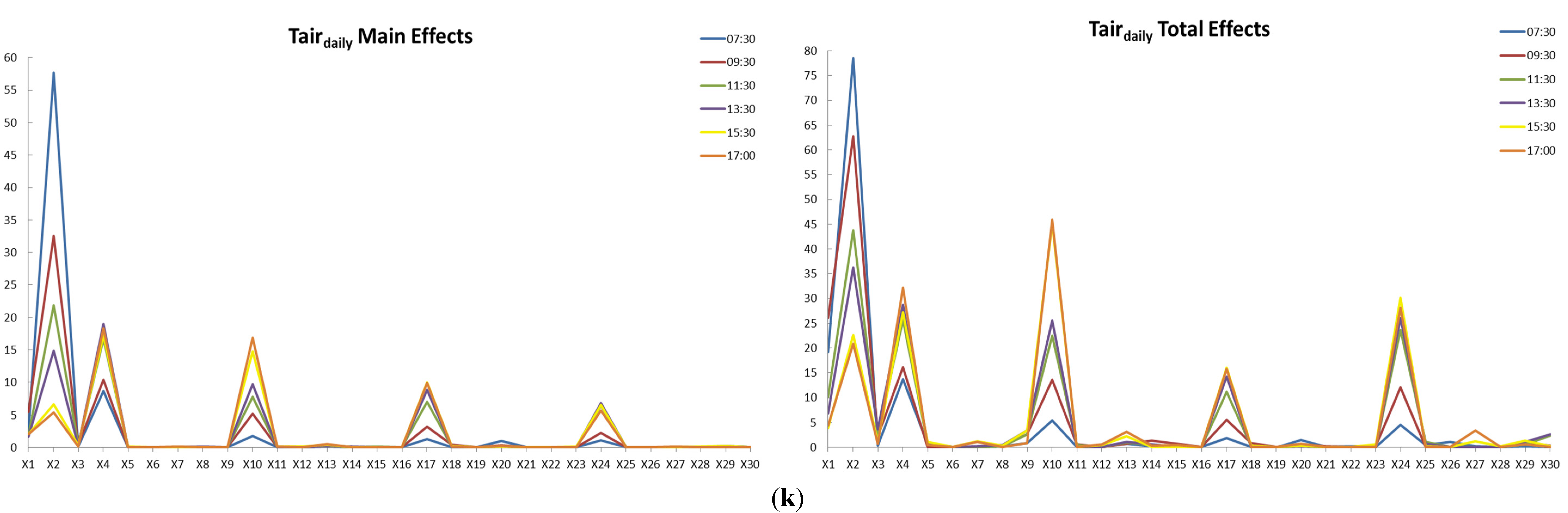
3.2.9. Parameter Sensitivity for ()
3.2.10. Parameter Sensitivity for ()
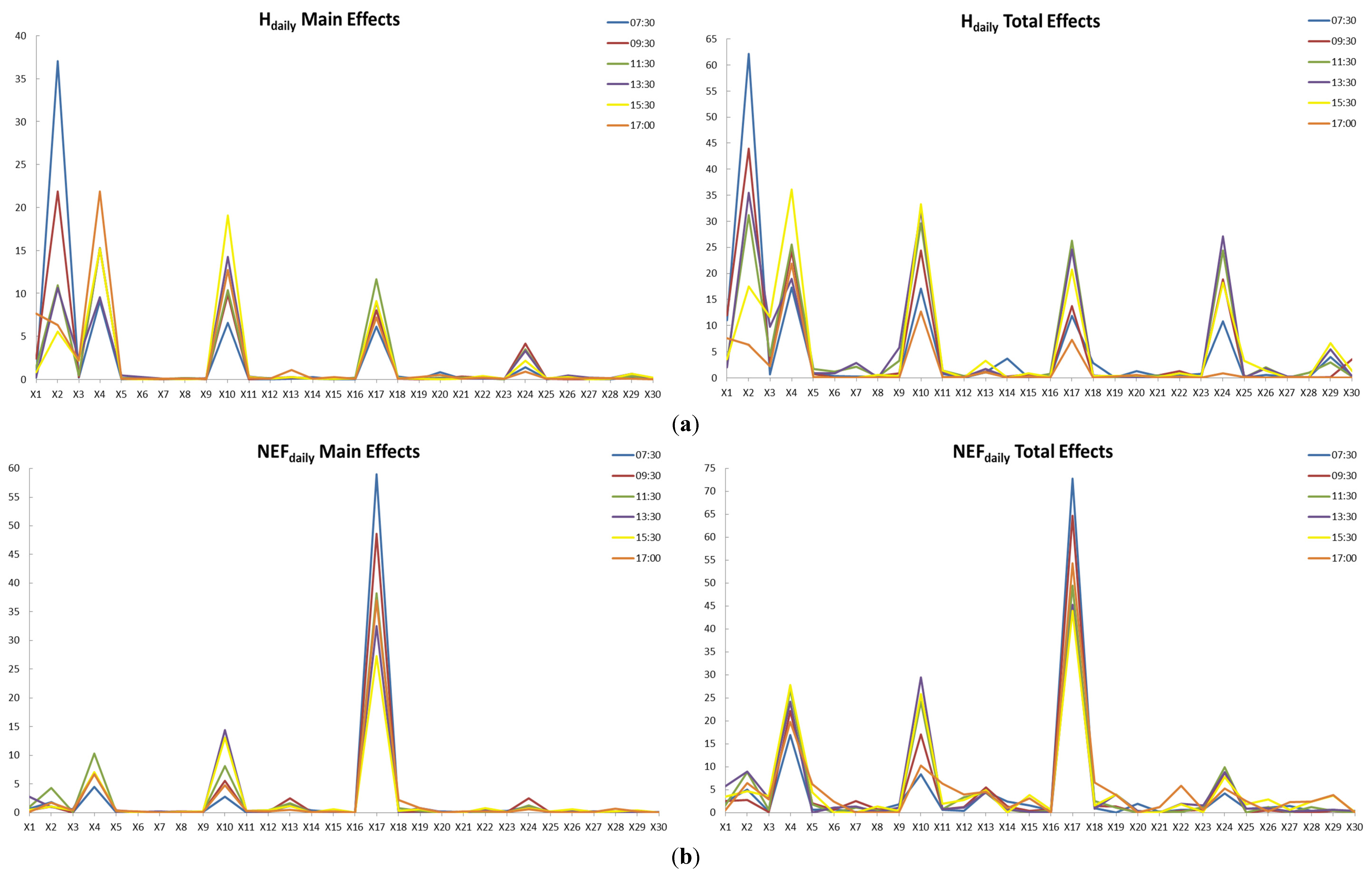


| Model Input | ||||||||||||||||||||||
|---|---|---|---|---|---|---|---|---|---|---|---|---|---|---|---|---|---|---|---|---|---|---|
| Main | Total | Main | Total | Main | Total | Main | Total | Main | Total | Main | Total | Main | Total | Main | Total | Main | Total | Main | Total | Main | Total | |
| X1 | 0.223 | 10.981 | 0.677 | 2.300 | 0.097 | 13.377 | 0.677 | 2.300 | 0.449 | 15.746 | - | - | 0.448 | 15.931 | 0.683 | 16.833 | 4.417 | 14.129 | 0.408 | 15.103 | 2.748 | 19.237 |
| X2 | 37.067 | 62.108 | 1.840 | 5.093 | 45.221 | 67.069 | 1.840 | 5.093 | 70.944 | 90.244 | - | - | 79.630 | 96.181 | 81.251 | 98.255 | 12.657 | 57.031 | 61.536 | 80.644 | 57.677 | 78.532 |
| X3 | 0.196 | 0.685 | 0.031 | 0.277 | 0.155 | 0.268 | 0.031 | 0.277 | 0.155 | 0.289 | - | - | 0.015 | 0.086 | 0.002 | 0.002 | 0.130 | 3.469 | 0.268 | 0.608 | 0.161 | 0.282 |
| X4 | 9.075 | 17.303 | 4.511 | 16.992 | 9.199 | 15.773 | 4.511 | 16.992 | 1.081 | 3.967 | - | - | 1.621 | 2.617 | 0.337 | 0.559 | 4.712 | 36.281 | 1.762 | 2.876 | 8.617 | 13.723 |
| X5 | 0.052 | 0.874 | 0.042 | 0.608 | 0.044 | 1.219 | 0.042 | 0.608 | 0.283 | 0.871 | - | - | 0.947 | 1.674 | 0.276 | 0.465 | 0.132 | 0.133 | 0.874 | 2.950 | 0.085 | 0.681 |
| X6 | 0.149 | 0.317 | 0.161 | 0.768 | 0.152 | 1.726 | 0.161 | 0.768 | 0.040 | 0.076 | - | - | 0.012 | 0.043 | 0.003 | 0.003 | 0.299 | 1.962 | 0.006 | 0.006 | 0.039 | 0.073 |
| X7 | 0.040 | 0.259 | 0.044 | 0.106 | 0.058 | 0.943 | 0.044 | 0.106 | 0.011 | 0.012 | - | - | 0.012 | 0.054 | 0.002 | 0.002 | 0.612 | 2.632 | 0.016 | 0.214 | 0.023 | 0.024 |
| X8 | 0.126 | 0.260 | 0.112 | 0.546 | 0.041 | 0.173 | 0.112 | 0.546 | 0.021 | 0.625 | - | - | 0.009 | 0.042 | 0.005 | 0.005 | 0.548 | 6.285 | 0.015 | 0.320 | 0.020 | 0.220 |
| X9 | 0.109 | 0.182 | 0.085 | 1.837 | 0.051 | 1.079 | 0.085 | 1.837 | 0.013 | 0.014 | - | - | 0.002 | 0.002 | 0.005 | 0.016 | 0.602 | 1.337 | 0.029 | 0.255 | 0.064 | 0.875 |
| X10 | 6.544 | 17.086 | 2.803 | 8.331 | 0.085 | 0.522 | 2.803 | 8.331 | 0.659 | 2.426 | - | - | 0.073 | 0.272 | 0.001 | 0.002 | 0.161 | 0.466 | 0.083 | 0.169 | 1.792 | 5.380 |
| X11 | 0.032 | 0.725 | 0.046 | 0.594 | 0.181 | 1.587 | 0.046 | 0.594 | 0.177 | 0.737 | - | - | 0.012 | 0.052 | 0.002 | 0.002 | 0.094 | 0.095 | 0.016 | 0.017 | 0.057 | 0.135 |
| X12 | 0.031 | 0.032 | 0.200 | 0.438 | 0.047 | 0.061 | 0.200 | 0.438 | 0.012 | 0.013 | - | - | 0.002 | 0.038 | 0.002 | 0.002 | 0.122 | 0.124 | 0.011 | 0.017 | 0.024 | 0.210 |
| X13 | 0.117 | 1.034 | 1.159 | 4.510 | 0.431 | 1.998 | 1.159 | 4.510 | 0.034 | 0.296 | - | - | 0.009 | 0.009 | 0.002 | 0.004 | 0.372 | 5.254 | 0.020 | 0.365 | 0.182 | 0.706 |
| X14 | 0.289 | 3.715 | 0.441 | 2.478 | 0.030 | 0.031 | 0.441 | 2.478 | 0.126 | 1.181 | - | - | 0.002 | 0.002 | 0.002 | 0.002 | 0.122 | 0.123 | 0.009 | 0.009 | 0.041 | 0.202 |
| X15 | 0.032 | 0.033 | 0.109 | 1.613 | 0.031 | 0.032 | 0.109 | 1.613 | 0.011 | 0.052 | - | - | 0.004 | 0.004 | 0.004 | 0.005 | 0.149 | 0.150 | 0.017 | 0.018 | 0.036 | 0.066 |
| X16 | 0.029 | 0.030 | 0.054 | 0.491 | 0.030 | 0.874 | 0.054 | 0.491 | 0.045 | 0.104 | - | - | 0.002 | 0.002 | 0.003 | 0.004 | 0.351 | 9.540 | 0.009 | 0.039 | 0.012 | 0.013 |
| X17 | 6.098 | 11.808 | 59.701 | 72.792 | 14.473 | 22.696 | 59.701 | 72.792 | 2.768 | 3.932 | - | - | 0.167 | 0.342 | 0.002 | 0.002 | 1.562 | 9.491 | 10.006 | 14.817 | 1.304 | 1.815 |
| X18 | 0.363 | 2.849 | 0.077 | 1.026 | 0.156 | 0.510 | 0.077 | 1.026 | 0.056 | 0.331 | - | - | 0.011 | 0.080 | 0.004 | 0.052 | 0.357 | 1.511 | 0.015 | 0.023 | 0.060 | 0.095 |
| X19 | 0.049 | 0.050 | 0.047 | 0.048 | 0.044 | 0.046 | 0.047 | 0.048 | 0.036 | 0.198 | - | - | 0.011 | 0.011 | 0.002 | 0.002 | 0.601 | 7.538 | 0.046 | 0.082 | 0.011 | 0.012 |
| X20 | 0.865 | 1.324 | 0.217 | 1.936 | 0.573 | 1.733 | 0.217 | 1.936 | 0.524 | 1.132 | - | - | 0.031 | 0.047 | 0.001 | 0.002 | 1.634 | 28.113 | 1.423 | 2.635 | 1.013 | 1.433 |
| X21 | 0.065 | 0.376 | 0.113 | 0.146 | 0.062 | 0.063 | 0.113 | 0.146 | 0.014 | 0.015 | - | - | 0.002 | 0.002 | 0.001 | 0.001 | 0.143 | 0.145 | 0.025 | 0.025 | 0.021 | 0.022 |
| X22 | 0.220 | 0.411 | 0.181 | 0.636 | 0.056 | 0.113 | 0.181 | 0.636 | 0.029 | 0.091 | - | - | 0.009 | 0.023 | 0.001 | 0.001 | 0.883 | 3.117 | 1.990 | 2.698 | 0.058 | 0.165 |
| X23 | 0.069 | 0.752 | 0.290 | 0.591 | 0.131 | 0.244 | 0.290 | 0.591 | 0.026 | 0.096 | - | - | 0.003 | 0.003 | 0.001 | 0.001 | 0.126 | 0.128 | 0.008 | 0.009 | 0.020 | 0.020 |
| X24 | 1.388 | 10.808 | 1.067 | 4.189 | 0.041 | 0.042 | 1.067 | 4.189 | 0.353 | 1.590 | - | - | 0.020 | 0.055 | 0.002 | 0.002 | 0.293 | 9.576 | 0.012 | 0.089 | 1.069 | 4.544 |
| X25 | 0.070 | 0.071 | 0.046 | 0.846 | 0.059 | 1.396 | 0.046 | 0.846 | 0.020 | 0.021 | - | - | 0.006 | 0.006 | 0.004 | 0.004 | 0.130 | 0.131 | 0.010 | 0.061 | 0.060 | 0.455 |
| X26 | 0.100 | 0.557 | 0.053 | 1.088 | 0.032 | 0.140 | 0.053 | 1.088 | 0.011 | 0.011 | - | - | 0.002 | 0.002 | 0.013 | 0.327 | 0.297 | 10.127 | 0.026 | 0.158 | 0.042 | 1.124 |
| X27 | 0.035 | 0.192 | 0.182 | 1.504 | 0.029 | 0.524 | 0.182 | 1.504 | 0.027 | 0.180 | - | - | 0.003 | 0.017 | 0.003 | 0.070 | 0.153 | 0.154 | 0.007 | 0.007 | 0.020 | 0.186 |
| X28 | 0.027 | 0.144 | 0.084 | 0.438 | 0.064 | 0.065 | 0.084 | 0.438 | 0.029 | 0.489 | - | - | 0.021 | 0.066 | 0.035 | 0.699 | 0.234 | 7.745 | 0.018 | 0.045 | 0.017 | 0.092 |
| X29 | 0.263 | 4.007 | 0.111 | 0.623 | 0.017 | 0.071 | 0.111 | 0.623 | 0.103 | 0.454 | - | - | 0.009 | 0.048 | 0.002 | 0.069 | 0.095 | 0.096 | 0.007 | 0.007 | 0.018 | 0.253 |
| X30 | 0.037 | 0.366 | 0.029 | 0.030 | 0.027 | 0.548 | 0.029 | 0.030 | 0.014 | 0.020 | - | - | 0.006 | 0.045 | 0.041 | 0.936 | 0.239 | 0.240 | 0.026 | 0.959 | 0.019 | 0.061 |
| ME | 63.762 | 74.513 | 71.617 | 74.513 | 78.072 | 0.000 | 83.097 | 82.694 | 32.228 | 78.700 | 75.310 | |||||||||||
| 1st | 25.383 | 19.311 | 22.723 | 19.311 | 19.114 | 0.000 | 16.132 | 16.468 | 33.336 | 17.933 | 19.752 | |||||||||||
| >1st | 10.855 | 6.176 | 5.660 | 6.176 | 2.814 | 0.770 | 0.838 | 34.436 | 3.367 | 4.938 | ||||||||||||
| Model Input | ||||||||||||||||||||||
|---|---|---|---|---|---|---|---|---|---|---|---|---|---|---|---|---|---|---|---|---|---|---|
| Main | Total | Main | Total | Main | Total | Main | Total | Main | Total | Main | Total | Main | Total | Main | Total | Main | Total | Main | Total | Main | Total | |
| X1 | 2.422 | 11.902 | 0.459 | 2.535 | 2.359 | 13.014 | 0.459 | 2.535 | 5.191 | 20.304 | 0.003 | 0.016 | 8.748 | 24.370 | 8.502 | 24.407 | 0.223 | 11.277 | 3.229 | 15.065 | 5.527 | 26.101 |
| X2 | 21.855 | 43.971 | 1.099 | 2.732 | 48.237 | 64.631 | 1.099 | 2.732 | 55.060 | 74.602 | 0.010 | 0.030 | 65.722 | 82.586 | 73.083 | 89.748 | 21.633 | 50.293 | 47.624 | 64.497 | 32.589 | 62.716 |
| X3 | 0.253 | 2.830 | 0.023 | 0.125 | 0.086 | 0.296 | 0.023 | 0.125 | 0.104 | 0.496 | 0.004 | 0.006 | 0.047 | 0.145 | 0.002 | 0.002 | 0.103 | 0.519 | 0.299 | 0.901 | 0.419 | 2.259 |
| X4 | 15.264 | 24.290 | 6.872 | 22.167 | 9.751 | 16.426 | 6.872 | 22.167 | 3.835 | 7.150 | 0.018 | 0.021 | 4.300 | 5.563 | 0.645 | 0.837 | 12.249 | 24.385 | 1.205 | 2.843 | 10.365 | 16.069 |
| X5 | 0.081 | 0.717 | 0.388 | 2.036 | 0.154 | 1.321 | 0.388 | 2.036 | 0.218 | 1.276 | 0.001 | 0.001 | 1.753 | 2.680 | 0.642 | 0.845 | 0.272 | 0.690 | 2.224 | 3.962 | 0.063 | 0.065 |
| X6 | 0.036 | 0.038 | 0.142 | 0.627 | 0.014 | 0.070 | 0.142 | 0.627 | 0.033 | 0.104 | 0.002 | 0.002 | 0.008 | 0.043 | 0.006 | 0.013 | 0.279 | 1.503 | 0.007 | 0.007 | 0.035 | 0.037 |
| X7 | 0.035 | 0.037 | 0.164 | 2.520 | 0.044 | 0.308 | 0.164 | 2.520 | 0.011 | 0.012 | 0.007 | 0.011 | 0.005 | 0.005 | 0.003 | 0.004 | 0.164 | 1.853 | 0.020 | 0.021 | 0.027 | 0.028 |
| X8 | 0.168 | 0.307 | 0.206 | 0.794 | 0.018 | 0.220 | 0.206 | 0.794 | 0.019 | 0.365 | 0.004 | 0.035 | 0.006 | 0.006 | 0.004 | 0.004 | 0.078 | 0.221 | 0.017 | 0.222 | 0.093 | 0.345 |
| X9 | 0.046 | 0.891 | 0.127 | 0.347 | 0.021 | 0.022 | 0.127 | 0.347 | 0.015 | 0.016 | 0.003 | 0.004 | 0.004 | 0.043 | 0.004 | 0.004 | 0.098 | 1.145 | 0.008 | 0.009 | 0.070 | 2.617 |
| X10 | 9.864 | 24.417 | 5.596 | 17.024 | 0.008 | 0.009 | 5.596 | 17.024 | 1.714 | 4.590 | 0.003 | 0.008 | 0.209 | 0.901 | 0.001 | 0.001 | 4.565 | 14.159 | 0.144 | 0.211 | 5.229 | 13.575 |
| X11 | 0.043 | 0.045 | 0.221 | 0.741 | 0.107 | 0.428 | 0.221 | 0.741 | 0.077 | 0.179 | 0.001 | 0.002 | 0.030 | 0.074 | 0.002 | 0.002 | 0.097 | 1.230 | 0.052 | 0.052 | 0.032 | 0.586 |
| X12 | 0.117 | 0.156 | 0.109 | 1.181 | 0.106 | 0.530 | 0.109 | 1.181 | 0.012 | 0.025 | 0.002 | 0.002 | 0.003 | 0.003 | 0.002 | 0.002 | 0.090 | 0.234 | 0.006 | 0.007 | 0.048 | 0.110 |
| X13 | 0.259 | 1.148 | 2.476 | 5.510 | 0.899 | 1.866 | 2.476 | 5.510 | 0.101 | 0.485 | 0.013 | 0.024 | 0.016 | 0.038 | 0.005 | 0.011 | 0.172 | 2.211 | 0.005 | 0.005 | 0.292 | 0.727 |
| X14 | 0.082 | 0.217 | 0.133 | 1.374 | 0.026 | 0.043 | 0.133 | 1.374 | 0.132 | 1.169 | 0.003 | 0.013 | 0.006 | 0.049 | 0.002 | 0.003 | 0.572 | 4.976 | 0.014 | 0.014 | 0.061 | 1.329 |
| X15 | 0.154 | 0.638 | 0.053 | 0.348 | 0.026 | 0.114 | 0.053 | 0.348 | 0.037 | 0.146 | 0.001 | 0.002 | 0.009 | 0.038 | 0.004 | 0.009 | 0.062 | 0.063 | 0.018 | 0.019 | 0.084 | 0.730 |
| X16 | 0.119 | 0.249 | 0.079 | 0.732 | 0.022 | 0.201 | 0.079 | 0.732 | 0.050 | 0.134 | 0.002 | 0.002 | 0.011 | 0.019 | 0.005 | 0.005 | 0.071 | 0.072 | 0.021 | 0.022 | 0.019 | 0.021 |
| X17 | 8.010 | 13.751 | 48.648 | 64.684 | 15.936 | 23.062 | 48.648 | 64.684 | 8.201 | 11.399 | 98.234 | 98.961 | 1.043 | 1.539 | 0.002 | 0.003 | 8.601 | 12.186 | 23.559 | 28.966 | 3.201 | 5.505 |
| X18 | 0.072 | 0.073 | 0.168 | 1.487 | 0.182 | 0.356 | 0.168 | 1.487 | 0.134 | 0.372 | 0.107 | 0.152 | 0.009 | 0.033 | 0.011 | 0.105 | 0.189 | 3.306 | 0.026 | 0.218 | 0.437 | 0.799 |
| X19 | 0.042 | 0.043 | 0.183 | 1.398 | 0.177 | 0.642 | 0.183 | 1.398 | 0.024 | 0.240 | 0.212 | 0.394 | 0.005 | 0.006 | 0.002 | 0.002 | 0.123 | 0.124 | 0.007 | 0.008 | 0.025 | 0.081 |
| X20 | 0.059 | 0.061 | 0.070 | 0.097 | 0.083 | 0.439 | 0.070 | 0.097 | 0.433 | 0.588 | 0.003 | 0.009 | 0.060 | 0.085 | 0.002 | 0.002 | 0.337 | 0.551 | 0.750 | 0.975 | 0.366 | 0.587 |
| X21 | 0.314 | 0.465 | 0.035 | 0.036 | 0.056 | 0.173 | 0.035 | 0.036 | 0.053 | 0.088 | 0.006 | 0.014 | 0.014 | 0.032 | 0.003 | 0.013 | 0.457 | 1.016 | 0.009 | 0.010 | 0.051 | 0.148 |
| X22 | 0.226 | 1.317 | 0.095 | 0.350 | 0.026 | 0.183 | 0.095 | 0.350 | 0.038 | 0.227 | 0.002 | 0.002 | 0.017 | 0.034 | 0.001 | 0.001 | 0.515 | 0.934 | 0.802 | 1.132 | 0.030 | 0.138 |
| X23 | 0.027 | 0.028 | 0.110 | 0.634 | 0.013 | 0.013 | 0.110 | 0.634 | 0.011 | 0.168 | 0.004 | 0.004 | 0.013 | 0.029 | 0.002 | 0.002 | 0.217 | 1.702 | 0.057 | 0.243 | 0.045 | 0.392 |
| X24 | 4.133 | 18.819 | 2.492 | 8.728 | 0.079 | 0.477 | 2.492 | 8.728 | 0.882 | 2.265 | 0.002 | 0.006 | 0.178 | 0.405 | 0.002 | 0.002 | 4.110 | 18.005 | 0.101 | 0.281 | 2.246 | 12.023 |
| X25 | 0.056 | 0.397 | 0.031 | 0.032 | 0.020 | 0.238 | 0.031 | 0.032 | 0.021 | 0.164 | 0.005 | 0.007 | 0.005 | 0.019 | 0.003 | 0.003 | 0.117 | 1.245 | 0.024 | 0.542 | 0.039 | 0.041 |
| X26 | 0.043 | 0.044 | 0.032 | 0.531 | 0.017 | 0.017 | 0.032 | 0.531 | 0.016 | 0.017 | 0.007 | 0.196 | 0.010 | 0.010 | 0.012 | 0.024 | 0.136 | 3.734 | 0.209 | 0.299 | 0.035 | 0.036 |
| X27 | 0.032 | 0.033 | 0.040 | 0.115 | 0.019 | 0.084 | 0.040 | 0.115 | 0.010 | 0.011 | 0.027 | 0.472 | 0.002 | 0.003 | 0.006 | 0.145 | 0.693 | 3.809 | 0.007 | 0.008 | 0.018 | 0.019 |
| X28 | 0.065 | 0.067 | 0.046 | 0.051 | 0.013 | 0.019 | 0.046 | 0.051 | 0.038 | 0.093 | 0.022 | 0.565 | 0.018 | 0.032 | 0.019 | 0.569 | 0.196 | 0.197 | 0.016 | 0.017 | 0.034 | 0.042 |
| X29 | 0.063 | 0.119 | 0.147 | 0.414 | 0.027 | 0.080 | 0.147 | 0.414 | 0.191 | 0.325 | 0.029 | 0.517 | 0.009 | 0.066 | 0.006 | 0.212 | 0.246 | 4.877 | 0.023 | 0.128 | 0.157 | 0.851 |
| X30 | 0.174 | 3.576 | 0.051 | 0.052 | 0.020 | 0.461 | 0.051 | 0.052 | 0.044 | 0.321 | 0.036 | 0.579 | 0.007 | 0.244 | 0.049 | 0.926 | 0.086 | 0.761 | 0.126 | 2.703 | 0.036 | 0.356 |
| ME | 64.115 | 70.296 | 78.545 | 70.296 | 76.708 | 98.771 | 82.266 | 83.034 | 56.751 | 80.611 | 61.674 | |||||||||||
| 1st | 24.063 | 21.507 | 17.728 | 21.507 | 19.828 | 0.591 | 16.550 | 16.195 | 24.649 | 16.012 | 29.931 | |||||||||||
| >1st | 11.822 | 8.197 | 3.726 | 8.197 | 3.464 | 0.638 | 1.184 | 0.772 | 18.601 | 3.377 | 8.395 | |||||||||||
| Model Input | ||||||||||||||||||||||
|---|---|---|---|---|---|---|---|---|---|---|---|---|---|---|---|---|---|---|---|---|---|---|
| Main | Total | Main | Total | Main | Total | Main | Total | Main | Total | Main | Total | Main | Total | Main | Total | Main | Total | Main | Total | Main | Total | |
| X1 | 1.388 | 3.078 | 0.991 | 1.613 | 7.969 | 16.245 | 0.991 | 1.613 | 12.676 | 24.032 | 17.129 | 29.450 | 20.294 | 31.964 | 24.194 | 37.021 | 1.829 | 9.768 | 8.000 | 17.326 | 1.846 | 10.150 |
| X2 | 10.944 | 31.147 | 4.283 | 8.882 | 36.024 | 51.870 | 4.283 | 8.883 | 34.857 | 52.048 | 28.462 | 50.207 | 50.095 | 63.626 | 59.032 | 72.365 | 22.227 | 44.020 | 30.660 | 44.439 | 21.877 | 43.797 |
| X3 | 0.469 | 4.245 | 0.130 | 0.610 | 0.066 | 0.825 | 0.130 | 0.610 | 0.031 | 0.150 | 1.278 | 4.853 | 0.016 | 0.353 | 0.004 | 0.068 | 0.354 | 2.429 | 0.562 | 2.150 | 0.411 | 2.482 |
| X4 | 15.239 | 25.509 | 10.362 | 26.932 | 8.132 | 16.975 | 10.362 | 26.932 | 5.586 | 10.606 | 0.704 | 6.702 | 7.161 | 8.916 | 1.480 | 2.035 | 16.437 | 25.228 | 2.202 | 4.227 | 16.655 | 25.647 |
| X5 | 0.135 | 1.710 | 0.060 | 1.824 | 0.184 | 0.709 | 0.060 | 1.824 | 0.049 | 1.462 | 12.028 | 20.080 | 2.060 | 3.357 | 1.396 | 1.828 | 0.071 | 0.699 | 4.340 | 6.618 | 0.071 | 0.672 |
| X6 | 0.142 | 1.136 | 0.032 | 0.034 | 0.027 | 0.028 | 0.032 | 0.034 | 0.048 | 0.177 | 0.030 | 0.151 | 0.014 | 0.094 | 0.003 | 0.025 | 0.020 | 0.022 | 0.011 | 0.012 | 0.020 | 0.022 |
| X7 | 0.090 | 2.166 | 0.065 | 1.086 | 0.049 | 0.855 | 0.065 | 1.086 | 0.028 | 0.029 | 0.054 | 0.198 | 0.010 | 0.015 | 0.002 | 0.002 | 0.046 | 0.091 | 0.043 | 0.074 | 0.037 | 0.039 |
| X8 | 0.120 | 0.262 | 0.060 | 0.544 | 0.031 | 0.181 | 0.060 | 0.544 | 0.020 | 0.021 | 0.065 | 0.474 | 0.008 | 0.008 | 0.002 | 0.003 | 0.106 | 0.228 | 0.014 | 0.096 | 0.102 | 0.200 |
| X9 | 0.093 | 3.309 | 0.093 | 0.120 | 0.098 | 0.898 | 0.093 | 0.120 | 0.149 | 1.703 | 0.032 | 0.222 | 0.029 | 0.465 | 0.002 | 0.002 | 0.066 | 2.760 | 0.010 | 0.064 | 0.067 | 2.669 |
| X10 | 10.357 | 29.664 | 8.155 | 24.214 | 0.015 | 0.016 | 8.155 | 24.214 | 3.293 | 7.415 | 0.803 | 2.066 | 0.427 | 1.234 | 0.001 | 0.001 | 8.206 | 22.483 | 0.123 | 0.344 | 7.832 | 22.447 |
| X11 | 0.275 | 1.401 | 0.308 | 0.759 | 0.350 | 0.677 | 0.308 | 0.759 | 0.127 | 0.432 | 0.177 | 2.093 | 0.021 | 0.095 | 0.003 | 0.003 | 0.043 | 0.424 | 0.022 | 0.190 | 0.044 | 0.500 |
| X12 | 0.137 | 0.306 | 0.442 | 3.400 | 0.065 | 0.091 | 0.442 | 3.400 | 0.026 | 0.027 | 0.033 | 0.034 | 0.006 | 0.007 | 0.002 | 0.003 | 0.043 | 0.045 | 0.010 | 0.011 | 0.058 | 0.060 |
| X13 | 0.158 | 1.041 | 1.653 | 4.295 | 1.546 | 2.699 | 1.652 | 4.295 | 0.609 | 0.922 | 0.151 | 0.490 | 0.134 | 0.203 | 0.001 | 0.001 | 0.263 | 0.955 | 0.019 | 0.019 | 0.247 | 0.929 |
| X14 | 0.088 | 0.090 | 0.155 | 0.599 | 0.037 | 0.052 | 0.155 | 0.599 | 0.074 | 0.155 | 0.131 | 0.174 | 0.013 | 0.066 | 0.002 | 0.002 | 0.115 | 0.448 | 0.051 | 0.070 | 0.097 | 0.395 |
| X15 | 0.037 | 0.039 | 0.025 | 0.026 | 0.041 | 0.042 | 0.025 | 0.026 | 0.070 | 0.506 | 0.030 | 0.031 | 0.024 | 0.077 | 0.006 | 0.006 | 0.110 | 0.219 | 0.054 | 0.305 | 0.122 | 0.260 |
| X16 | 0.242 | 0.717 | 0.042 | 0.477 | 0.021 | 0.422 | 0.042 | 0.477 | 0.168 | 0.563 | 0.042 | 0.648 | 0.021 | 0.057 | 0.002 | 0.002 | 0.052 | 0.054 | 0.024 | 0.079 | 0.055 | 0.057 |
| X17 | 11.669 | 26.284 | 38.199 | 49.518 | 17.567 | 27.166 | 38.200 | 49.518 | 16.911 | 21.465 | 3.563 | 7.129 | 3.554 | 5.219 | 0.001 | 0.002 | 6.847 | 10.961 | 34.463 | 38.899 | 7.010 | 11.169 |
| X18 | 0.099 | 0.101 | 0.835 | 2.507 | 0.251 | 0.707 | 0.835 | 2.507 | 0.095 | 0.159 | 0.054 | 1.229 | 0.071 | 0.160 | 0.005 | 0.005 | 0.176 | 0.233 | 0.021 | 0.195 | 0.143 | 0.145 |
| X19 | 0.054 | 0.056 | 0.286 | 1.056 | 0.643 | 1.300 | 0.286 | 1.055 | 0.056 | 0.090 | 0.284 | 0.735 | 0.010 | 0.010 | 0.002 | 0.002 | 0.029 | 0.031 | 0.039 | 0.055 | 0.033 | 0.035 |
| X20 | 0.190 | 0.308 | 0.036 | 0.038 | 0.098 | 0.538 | 0.036 | 0.038 | 0.346 | 0.347 | 0.749 | 1.608 | 0.083 | 0.125 | 0.004 | 0.004 | 0.171 | 0.253 | 0.580 | 0.749 | 0.167 | 0.256 |
| X21 | 0.228 | 0.487 | 0.072 | 0.234 | 0.029 | 0.030 | 0.072 | 0.234 | 0.043 | 0.044 | 0.035 | 0.037 | 0.032 | 0.050 | 0.002 | 0.002 | 0.118 | 0.168 | 0.012 | 0.013 | 0.105 | 0.137 |
| X22 | 0.119 | 0.121 | 0.045 | 0.194 | 0.130 | 0.841 | 0.045 | 0.194 | 0.043 | 0.449 | 0.055 | 0.057 | 0.016 | 0.043 | 0.003 | 0.003 | 0.099 | 0.100 | 0.623 | 0.884 | 0.094 | 0.096 |
| X23 | 0.052 | 0.054 | 0.066 | 1.239 | 0.032 | 0.378 | 0.066 | 1.239 | 0.042 | 0.718 | 0.124 | 0.653 | 0.009 | 0.025 | 0.002 | 0.002 | 0.026 | 0.165 | 0.020 | 0.116 | 0.025 | 0.081 |
| X24 | 3.509 | 24.425 | 1.318 | 9.913 | 0.222 | 0.707 | 1.318 | 9.913 | 0.853 | 2.332 | 1.391 | 4.019 | 0.285 | 0.745 | 0.002 | 0.003 | 6.475 | 23.542 | 0.295 | 0.565 | 6.465 | 23.644 |
| X25 | 0.049 | 0.051 | 0.075 | 0.076 | 0.044 | 0.552 | 0.075 | 0.076 | 0.051 | 1.067 | 0.061 | 1.551 | 0.010 | 0.129 | 0.002 | 0.002 | 0.040 | 0.926 | 0.020 | 0.482 | 0.042 | 1.070 |
| X26 | 0.264 | 2.020 | 0.050 | 1.240 | 0.079 | 0.625 | 0.050 | 1.240 | 0.087 | 0.368 | 0.051 | 0.052 | 0.030 | 0.059 | 0.004 | 0.004 | 0.053 | 0.055 | 0.093 | 0.094 | 0.047 | 0.049 |
| X27 | 0.043 | 0.045 | 0.026 | 0.028 | 0.032 | 0.909 | 0.026 | 0.028 | 0.017 | 0.018 | 0.053 | 0.330 | 0.005 | 0.005 | 0.001 | 0.001 | 0.039 | 0.041 | 0.013 | 0.121 | 0.031 | 0.033 |
| X28 | 0.072 | 1.019 | 0.224 | 1.261 | 0.044 | 0.882 | 0.224 | 1.261 | 0.049 | 0.321 | 0.374 | 2.540 | 0.035 | 0.075 | 0.003 | 0.062 | 0.068 | 0.070 | 0.011 | 0.103 | 0.082 | 0.084 |
| X29 | 0.402 | 2.995 | 0.118 | 0.404 | 0.028 | 0.866 | 0.118 | 0.404 | 0.344 | 1.024 | 0.103 | 2.105 | 0.058 | 0.289 | 0.018 | 0.456 | 0.204 | 0.631 | 0.071 | 1.911 | 0.206 | 0.585 |
| X30 | 0.074 | 0.199 | 0.052 | 0.099 | 0.285 | 5.121 | 0.052 | 0.099 | 0.096 | 0.781 | 0.042 | 0.661 | 0.036 | 0.276 | 0.045 | 0.707 | 0.085 | 2.490 | 0.041 | 1.448 | 0.071 | 2.333 |
| ME | 56.735 | 68.258 | 74.138 | 68.258 | 76.844 | 68.091 | 84.568 | 86.228 | 64.419 | 82.449 | 64.061 | |||||||||||
| 1st | 26.454 | 22.129 | 19.706 | 22.129 | 17.916 | 24.610 | 13.486 | 13.103 | 24.015 | 14.145 | 24.309 | |||||||||||
| >1st | 16.810 | 9.613 | 6.156 | 9.613 | 5.240 | 7.299 | 1.946 | 0.669 | 11.566 | 3.406 | 11.630 | |||||||||||
| Model Input | ||||||||||||||||||||||
|---|---|---|---|---|---|---|---|---|---|---|---|---|---|---|---|---|---|---|---|---|---|---|
| Main | Total | Main | Total | Main | Total | Main | Total | Main | Total | Main | Total | Main | Total | Main | Total | Main | Total | Main | Total | Main | Total | |
| X1 | 0.258 | 2.032 | 2.803 | 5.790 | 8.858 | 19.630 | 2.803 | 5.790 | 20.980 | 29.266 | 0.006 | 0.071 | 16.772 | 30.006 | 26.631 | 39.252 | 1.490 | 5.756 | 13.191 | 21.469 | 1.640 | 6.882 |
| X2 | 10.624 | 35.532 | 1.030 | 9.012 | 35.301 | 53.735 | 1.030 | 9.013 | 21.225 | 36.278 | 0.023 | 0.200 | 53.241 | 69.238 | 56.339 | 69.652 | 14.958 | 34.670 | 15.409 | 26.075 | 14.860 | 36.216 |
| X3 | 2.452 | 9.758 | 0.596 | 3.090 | 4.080 | 9.987 | 0.596 | 3.090 | 0.748 | 2.825 | 0.007 | 0.033 | 0.148 | 0.781 | 0.006 | 0.117 | 0.136 | 2.498 | 2.554 | 4.786 | 0.234 | 3.582 |
| X4 | 9.532 | 18.998 | 6.972 | 24.273 | 4.941 | 12.899 | 6.972 | 24.273 | 1.475 | 4.057 | 0.135 | 0.214 | 5.083 | 6.425 | 1.499 | 2.017 | 18.585 | 26.920 | 3.934 | 7.646 | 19.015 | 28.712 |
| X5 | 0.464 | 0.874 | 0.091 | 0.092 | 0.199 | 1.030 | 0.091 | 0.092 | 0.599 | 3.824 | 0.009 | 0.013 | 1.038 | 2.121 | 1.537 | 1.992 | 0.100 | 1.907 | 6.479 | 10.285 | 0.053 | 0.883 |
| X6 | 0.273 | 0.916 | 0.112 | 1.139 | 0.055 | 0.792 | 0.112 | 1.139 | 0.144 | 0.446 | 0.002 | 0.002 | 0.053 | 0.208 | 0.002 | 0.002 | 0.046 | 0.048 | 0.027 | 0.078 | 0.023 | 0.025 |
| X7 | 0.115 | 2.859 | 0.208 | 1.302 | 0.059 | 0.874 | 0.207 | 1.302 | 0.062 | 0.831 | 0.007 | 0.186 | 0.015 | 0.306 | 0.002 | 0.003 | 0.054 | 0.361 | 0.030 | 0.425 | 0.060 | 0.150 |
| X8 | 0.049 | 0.051 | 0.074 | 0.185 | 0.086 | 0.785 | 0.074 | 0.185 | 0.030 | 0.437 | 0.003 | 0.067 | 0.012 | 0.303 | 0.004 | 0.004 | 0.049 | 0.144 | 0.015 | 0.090 | 0.126 | 0.461 |
| X9 | 0.167 | 5.809 | 0.079 | 1.099 | 0.063 | 0.183 | 0.079 | 1.099 | 0.039 | 0.040 | 0.003 | 0.072 | 0.012 | 0.120 | 0.003 | 0.005 | 0.065 | 2.668 | 0.014 | 0.014 | 0.076 | 3.422 |
| X10 | 14.255 | 32.134 | 14.389 | 29.439 | 0.117 | 0.518 | 14.389 | 29.438 | 4.707 | 9.977 | 0.003 | 0.003 | 0.615 | 1.355 | 0.001 | 0.001 | 10.440 | 29.640 | 0.363 | 1.035 | 9.662 | 25.566 |
| X11 | 0.317 | 1.007 | 0.242 | 0.725 | 0.037 | 0.102 | 0.242 | 0.725 | 0.043 | 0.160 | 0.002 | 0.016 | 0.013 | 0.075 | 0.004 | 0.076 | 0.131 | 0.331 | 0.017 | 0.072 | 0.045 | 0.047 |
| X12 | 0.093 | 0.187 | 0.122 | 1.117 | 0.263 | 2.013 | 0.122 | 1.117 | 0.049 | 0.670 | 0.003 | 0.040 | 0.009 | 0.049 | 0.003 | 0.004 | 0.070 | 0.072 | 0.014 | 0.014 | 0.059 | 0.060 |
| X13 | 0.146 | 1.703 | 1.283 | 4.497 | 2.142 | 4.133 | 1.283 | 4.497 | 1.150 | 1.912 | 0.015 | 0.049 | 0.211 | 0.407 | 0.002 | 0.002 | 0.210 | 1.041 | 0.022 | 0.023 | 0.259 | 1.049 |
| X14 | 0.117 | 0.119 | 0.119 | 0.735 | 0.052 | 0.757 | 0.119 | 0.735 | 0.114 | 0.514 | 0.002 | 0.009 | 0.020 | 0.553 | 0.002 | 0.002 | 0.143 | 1.673 | 0.047 | 0.193 | 0.173 | 0.526 |
| X15 | 0.090 | 0.155 | 0.061 | 0.125 | 0.029 | 0.031 | 0.061 | 0.125 | 0.034 | 0.501 | 0.003 | 0.004 | 0.018 | 0.018 | 0.011 | 0.012 | 0.052 | 0.054 | 0.023 | 0.177 | 0.062 | 0.064 |
| X16 | 0.084 | 0.289 | 0.079 | 0.080 | 0.040 | 0.932 | 0.079 | 0.080 | 0.033 | 0.310 | 0.002 | 0.007 | 0.009 | 0.131 | 0.002 | 0.002 | 0.062 | 0.064 | 0.034 | 0.125 | 0.051 | 0.053 |
| X17 | 8.990 | 24.616 | 32.567 | 45.266 | 10.622 | 18.004 | 32.566 | 45.266 | 20.525 | 29.487 | 90.535 | 92.266 | 4.073 | 5.626 | 0.002 | 0.002 | 8.729 | 13.153 | 38.568 | 43.511 | 8.820 | 14.172 |
| X18 | 0.109 | 0.498 | 0.105 | 0.889 | 0.316 | 1.342 | 0.105 | 0.889 | 0.259 | 0.570 | 0.538 | 0.751 | 0.021 | 0.160 | 0.005 | 0.005 | 0.151 | 0.153 | 0.036 | 0.471 | 0.108 | 0.110 |
| X19 | 0.055 | 0.195 | 0.816 | 3.912 | 1.046 | 3.413 | 0.816 | 3.912 | 0.176 | 0.473 | 5.818 | 7.871 | 0.038 | 0.184 | 0.004 | 0.005 | 0.032 | 0.034 | 0.098 | 0.199 | 0.033 | 0.035 |
| X20 | 0.083 | 0.085 | 0.119 | 0.345 | 0.031 | 0.033 | 0.119 | 0.345 | 0.284 | 0.528 | 0.002 | 0.002 | 0.024 | 0.049 | 0.003 | 0.003 | 0.282 | 0.434 | 0.546 | 0.826 | 0.170 | 0.253 |
| X21 | 0.078 | 0.080 | 0.045 | 0.047 | 0.069 | 0.070 | 0.045 | 0.047 | 0.124 | 0.189 | 0.005 | 0.205 | 0.023 | 0.036 | 0.002 | 0.002 | 0.238 | 0.387 | 0.054 | 0.093 | 0.101 | 0.139 |
| X22 | 0.104 | 0.106 | 0.483 | 1.933 | 0.054 | 0.648 | 0.483 | 1.933 | 0.042 | 0.864 | 0.003 | 0.003 | 0.028 | 0.074 | 0.003 | 0.003 | 0.059 | 0.061 | 0.456 | 0.726 | 0.069 | 0.071 |
| X23 | 0.053 | 0.055 | 0.117 | 1.628 | 0.074 | 1.136 | 0.117 | 1.628 | 0.047 | 0.421 | 0.003 | 0.003 | 0.034 | 0.203 | 0.004 | 0.004 | 0.039 | 1.174 | 0.013 | 0.014 | 0.028 | 0.082 |
| X24 | 3.333 | 27.149 | 0.891 | 8.897 | 0.427 | 0.891 | 0.891 | 8.897 | 1.345 | 5.067 | 0.002 | 0.004 | 0.373 | 0.921 | 0.002 | 0.002 | 6.458 | 25.824 | 0.687 | 1.472 | 6.839 | 26.038 |
| X25 | 0.052 | 0.054 | 0.059 | 0.836 | 0.058 | 0.799 | 0.059 | 0.836 | 0.076 | 1.494 | 0.006 | 0.006 | 0.018 | 0.068 | 0.003 | 0.003 | 0.050 | 0.187 | 0.023 | 0.889 | 0.040 | 0.746 |
| X26 | 0.470 | 1.851 | 0.324 | 1.013 | 0.096 | 0.896 | 0.324 | 1.013 | 0.205 | 0.668 | 0.005 | 0.005 | 0.033 | 0.270 | 0.005 | 0.005 | 0.080 | 1.766 | 0.026 | 0.027 | 0.052 | 0.054 |
| X27 | 0.200 | 0.235 | 0.181 | 0.305 | 0.114 | 0.942 | 0.181 | 0.305 | 0.116 | 0.162 | 0.025 | 0.350 | 0.041 | 0.076 | 0.001 | 0.001 | 0.045 | 0.047 | 0.093 | 0.151 | 0.034 | 0.036 |
| X28 | 0.123 | 0.125 | 0.064 | 0.425 | 0.184 | 0.328 | 0.064 | 0.426 | 0.055 | 0.056 | 0.012 | 0.309 | 0.014 | 0.015 | 0.002 | 0.007 | 0.060 | 0.062 | 0.026 | 0.026 | 0.068 | 0.070 |
| X29 | 0.645 | 5.418 | 0.075 | 0.621 | 0.202 | 1.538 | 0.075 | 0.621 | 0.368 | 0.935 | 0.004 | 0.006 | 0.155 | 0.676 | 0.038 | 0.895 | 0.304 | 1.427 | 0.060 | 0.779 | 0.270 | 1.088 |
| X30 | 0.102 | 0.252 | 0.154 | 0.342 | 0.289 | 0.452 | 0.154 | 0.342 | 0.033 | 0.330 | 0.093 | 1.139 | 0.014 | 0.015 | 0.057 | 0.926 | 0.055 | 0.489 | 0.028 | 0.328 | 0.075 | 2.602 |
| ME | 53.436 | 64.258 | 69.903 | 64.258 | 75.085 | 97.277 | 82.158 | 86.181 | 63.173 | 82.885 | 63.103 | |||||||||||
| 1st | 25.602 | 24.638 | 22.756 | 24.638 | 17.964 | 1.749 | 15.586 | 12.879 | 23.324 | 13.143 | 23.442 | |||||||||||
| >1st | 20.962 | 11.104 | 7.341 | 11.104 | 6.952 | 0.975 | 2.256 | 0.940 | 13.503 | 3.972 | 13.455 | |||||||||||
| Model Input | ||||||||||||||||||||||
|---|---|---|---|---|---|---|---|---|---|---|---|---|---|---|---|---|---|---|---|---|---|---|
| Main | Total | Main | Total | Main | Total | Main | Total | Main | Total | Main | Total | Main | Total | Main | Total | Main | Total | Main | Total | Main | Total | |
| X1 | 0.832 | 3.592 | 0.556 | 3.508 | 6.576 | 21.794 | 0.556 | 3.508 | 10.218 | 19.780 | 0.012 | 0.016 | 5.727 | 21.130 | 9.784 | 24.946 | 2.003 | 3.787 | 9.748 | 14.866 | 2.075 | 3.841 |
| X2 | 5.554 | 17.512 | 1.115 | 4.640 | 29.243 | 52.238 | 1.115 | 4.639 | 23.252 | 40.114 | 0.016 | 0.279 | 66.243 | 85.626 | 71.668 | 87.705 | 6.376 | 22.660 | 15.842 | 30.476 | 6.605 | 22.600 |
| X3 | 2.160 | 11.685 | 0.403 | 3.563 | 3.378 | 12.456 | 0.403 | 3.562 | 0.766 | 5.727 | 0.009 | 0.216 | 0.016 | 0.206 | 0.002 | 0.017 | 0.333 | 1.151 | 2.470 | 5.825 | 0.357 | 1.149 |
| X4 | 15.232 | 36.115 | 7.108 | 27.845 | 9.028 | 19.312 | 7.108 | 27.845 | 0.158 | 5.263 | 0.260 | 0.634 | 2.491 | 3.944 | 0.923 | 1.229 | 16.611 | 26.504 | 3.249 | 9.319 | 17.214 | 27.186 |
| X5 | 0.065 | 0.109 | 0.313 | 4.496 | 0.126 | 1.042 | 0.313 | 4.496 | 2.037 | 3.840 | 0.002 | 0.002 | 0.260 | 1.325 | 0.914 | 1.234 | 0.122 | 0.933 | 8.939 | 15.751 | 0.122 | 1.051 |
| X6 | 0.051 | 0.053 | 0.043 | 0.045 | 0.099 | 0.619 | 0.043 | 0.045 | 0.324 | 1.132 | 0.005 | 0.014 | 0.055 | 0.238 | 0.002 | 0.003 | 0.099 | 0.101 | 0.032 | 0.244 | 0.076 | 0.078 |
| X7 | 0.054 | 0.055 | 0.048 | 0.050 | 0.050 | 0.364 | 0.048 | 0.050 | 0.070 | 0.072 | 0.005 | 0.005 | 0.017 | 0.269 | 0.003 | 0.003 | 0.057 | 1.217 | 0.048 | 0.575 | 0.063 | 1.255 |
| X8 | 0.046 | 0.556 | 0.116 | 1.335 | 0.058 | 1.249 | 0.116 | 1.335 | 0.115 | 1.798 | 0.002 | 0.047 | 0.055 | 0.248 | 0.018 | 0.018 | 0.044 | 0.565 | 0.024 | 0.025 | 0.041 | 0.370 |
| X9 | 0.072 | 0.336 | 0.177 | 0.338 | 0.076 | 0.077 | 0.177 | 0.338 | 0.062 | 0.069 | 0.002 | 0.014 | 0.015 | 0.068 | 0.003 | 0.003 | 0.090 | 3.550 | 0.058 | 0.098 | 0.086 | 3.364 |
| X10 | 19.044 | 33.255 | 13.063 | 25.890 | 1.105 | 2.386 | 13.062 | 25.888 | 6.262 | 18.014 | 0.002 | 0.002 | 0.927 | 1.897 | 0.003 | 0.003 | 15.080 | 45.935 | 2.230 | 4.640 | 14.802 | 45.216 |
| X11 | 0.276 | 1.367 | 0.365 | 1.907 | 0.338 | 0.856 | 0.365 | 1.907 | 0.059 | 0.060 | 0.004 | 0.089 | 0.013 | 0.013 | 0.003 | 0.003 | 0.129 | 0.131 | 0.058 | 0.059 | 0.121 | 0.123 |
| X12 | 0.057 | 0.059 | 0.430 | 2.767 | 0.988 | 4.424 | 0.430 | 2.768 | 1.181 | 7.777 | 0.005 | 0.006 | 0.058 | 0.157 | 0.004 | 0.004 | 0.190 | 0.394 | 0.046 | 0.205 | 0.195 | 0.437 |
| X13 | 0.305 | 3.287 | 1.203 | 4.908 | 1.933 | 7.773 | 1.203 | 4.908 | 0.732 | 1.129 | 0.005 | 0.023 | 0.252 | 0.438 | 0.003 | 0.003 | 0.501 | 2.295 | 0.177 | 0.304 | 0.474 | 2.252 |
| X14 | 0.078 | 0.080 | 0.077 | 0.079 | 0.104 | 0.180 | 0.077 | 0.079 | 0.067 | 0.970 | 0.004 | 0.004 | 0.030 | 0.317 | 0.003 | 0.003 | 0.046 | 0.048 | 0.037 | 0.038 | 0.046 | 0.048 |
| X15 | 0.110 | 0.834 | 0.579 | 3.830 | 0.049 | 0.618 | 0.579 | 3.830 | 0.117 | 0.928 | 0.002 | 0.002 | 0.093 | 1.233 | 0.011 | 0.024 | 0.056 | 0.058 | 0.044 | 0.688 | 0.074 | 0.078 |
| X16 | 0.094 | 0.096 | 0.061 | 0.606 | 0.084 | 1.769 | 0.061 | 0.606 | 0.094 | 0.363 | 0.002 | 0.007 | 0.030 | 0.278 | 0.008 | 0.017 | 0.081 | 0.402 | 0.046 | 0.235 | 0.066 | 0.119 |
| X17 | 9.113 | 20.686 | 27.379 | 43.928 | 4.275 | 10.945 | 27.379 | 43.928 | 11.870 | 19.568 | 85.697 | 87.824 | 1.642 | 3.173 | 0.002 | 0.002 | 10.111 | 16.129 | 30.847 | 36.251 | 9.963 | 16.017 |
| X18 | 0.167 | 0.360 | 0.320 | 1.631 | 0.259 | 0.687 | 0.321 | 1.631 | 1.216 | 2.521 | 0.749 | 0.956 | 0.092 | 0.166 | 0.004 | 0.004 | 0.230 | 0.325 | 0.275 | 1.689 | 0.221 | 0.325 |
| X19 | 0.076 | 0.295 | 0.618 | 3.965 | 0.802 | 5.967 | 0.618 | 3.965 | 0.401 | 4.889 | 9.826 | 12.510 | 0.043 | 0.508 | 0.004 | 0.004 | 0.087 | 0.089 | 0.066 | 0.106 | 0.089 | 0.091 |
| X20 | 0.046 | 0.501 | 0.068 | 0.070 | 0.748 | 2.576 | 0.068 | 0.070 | 0.087 | 1.996 | 0.004 | 0.004 | 0.022 | 0.022 | 0.002 | 0.002 | 0.182 | 0.404 | 0.350 | 0.547 | 0.163 | 0.390 |
| X21 | 0.092 | 0.094 | 0.053 | 0.055 | 0.054 | 0.056 | 0.053 | 0.055 | 0.203 | 0.885 | 0.003 | 0.062 | 0.020 | 0.248 | 0.002 | 0.002 | 0.057 | 0.059 | 0.033 | 0.336 | 0.049 | 0.051 |
| X22 | 0.426 | 0.895 | 0.752 | 1.852 | 0.062 | 0.289 | 0.752 | 1.852 | 0.154 | 4.071 | 0.003 | 0.014 | 0.016 | 0.115 | 0.001 | 0.002 | 0.058 | 0.059 | 1.039 | 1.499 | 0.054 | 0.056 |
| X23 | 0.111 | 0.270 | 0.107 | 0.175 | 0.049 | 0.653 | 0.107 | 0.175 | 0.150 | 0.683 | 0.003 | 0.003 | 0.031 | 0.469 | 0.004 | 0.004 | 0.136 | 0.588 | 0.026 | 0.244 | 0.122 | 0.611 |
| X24 | 2.196 | 18.184 | 0.785 | 7.727 | 0.417 | 0.869 | 0.785 | 7.727 | 1.276 | 3.901 | 0.004 | 0.004 | 0.338 | 0.929 | 0.010 | 0.018 | 6.452 | 30.283 | 1.254 | 2.362 | 6.539 | 30.191 |
| X25 | 0.143 | 3.224 | 0.190 | 1.820 | 0.094 | 0.606 | 0.190 | 1.819 | 0.177 | 1.031 | 0.004 | 0.004 | 0.026 | 0.419 | 0.003 | 0.003 | 0.126 | 0.177 | 0.074 | 1.674 | 0.104 | 0.160 |
| X26 | 0.285 | 1.431 | 0.589 | 2.878 | 0.048 | 0.050 | 0.589 | 2.878 | 0.122 | 2.830 | 0.003 | 0.003 | 0.017 | 0.310 | 0.004 | 0.004 | 0.049 | 0.050 | 0.059 | 0.060 | 0.046 | 0.048 |
| X27 | 0.051 | 0.053 | 0.083 | 0.641 | 0.079 | 0.164 | 0.083 | 0.641 | 0.138 | 1.375 | 0.031 | 0.153 | 0.029 | 0.112 | 0.036 | 0.409 | 0.054 | 1.126 | 0.084 | 0.214 | 0.053 | 1.277 |
| X28 | 0.087 | 0.088 | 0.206 | 2.444 | 0.119 | 1.004 | 0.206 | 2.444 | 0.075 | 0.077 | 0.010 | 0.084 | 0.012 | 0.013 | 0.031 | 0.792 | 0.120 | 0.232 | 0.028 | 0.029 | 0.124 | 0.205 |
| X29 | 0.636 | 6.664 | 0.434 | 3.749 | 0.293 | 2.798 | 0.434 | 3.750 | 0.690 | 1.504 | 0.005 | 0.123 | 0.109 | 0.635 | 0.042 | 0.588 | 0.231 | 1.312 | 0.073 | 0.959 | 0.227 | 1.390 |
| X30 | 0.225 | 1.283 | 0.079 | 0.197 | 0.050 | 0.051 | 0.079 | 0.197 | 0.085 | 1.161 | 0.089 | 1.290 | 0.020 | 0.045 | 0.036 | 0.676 | 0.060 | 0.265 | 0.052 | 1.344 | 0.056 | 0.237 |
| ME | 57.688 | 57.322 | 60.584 | 57.322 | 62.160 | 96.767 | 78.699 | 83.533 | 59.772 | 77.308 | 60.230 | |||||||||||
| 1st | 25.812 | 30.833 | 27.707 | 30.833 | 25.027 | 2.249 | 18.477 | 15.467 | 23.448 | 16.058 | 23.141 | |||||||||||
| >1st | 16.500 | 11.845 | 11.709 | 11.845 | 12.813 | 0.985 | 2.824 | 1.000 | 16.779 | 6.635 | 16.630 | |||||||||||
| Model Input | ||||||||||||||||||||||
|---|---|---|---|---|---|---|---|---|---|---|---|---|---|---|---|---|---|---|---|---|---|---|
| Main | Total | Main | Total | Main | Total | Main | Total | Main | Total | Main | Total | Main | Total | Main | Total | Main | Total | Main | Total | Main | Total | |
| X1 | 7.612 | 18.549 | 0.162 | 0.538 | 8.754 | 21.342 | 0.162 | 0.538 | 4.896 | 21.217 | 0.007 | 0.042 | 1.221 | 16.581 | 2.602 | 18.722 | 1.957 | 4.418 | 5.208 | 18.547 | 2.052 | 4.469 |
| X2 | 6.335 | 20.092 | 1.719 | 6.424 | 17.968 | 31.767 | 1.719 | 6.424 | 45.527 | 70.714 | 0.038 | 0.408 | 74.092 | 92.036 | 78.891 | 95.926 | 5.366 | 21.389 | 41.956 | 63.756 | 5.383 | 20.810 |
| X3 | 2.261 | 12.804 | 0.389 | 2.852 | 1.853 | 9.565 | 0.389 | 2.852 | 0.656 | 5.953 | 0.022 | 0.310 | 0.023 | 0.299 | 0.003 | 0.022 | 0.138 | 0.645 | 0.706 | 2.838 | 0.147 | 0.698 |
| X4 | 21.855 | 34.570 | 6.656 | 19.775 | 21.241 | 38.235 | 6.656 | 19.775 | 0.432 | 11.528 | 0.378 | 0.776 | 2.094 | 3.924 | 0.403 | 0.603 | 17.681 | 32.486 | 0.394 | 5.578 | 18.287 | 32.124 |
| X5 | 0.112 | 3.092 | 0.279 | 6.266 | 0.211 | 2.193 | 0.279 | 6.266 | 1.132 | 6.202 | 0.013 | 0.037 | 0.163 | 0.923 | 0.472 | 0.682 | 0.095 | 0.396 | 5.017 | 10.763 | 0.103 | 0.504 |
| X6 | 0.069 | 0.418 | 0.177 | 2.387 | 0.036 | 0.037 | 0.177 | 2.387 | 0.086 | 0.215 | 0.003 | 0.071 | 0.031 | 0.051 | 0.002 | 0.002 | 0.033 | 0.034 | 0.021 | 0.120 | 0.035 | 0.036 |
| X7 | 0.079 | 0.081 | 0.074 | 0.076 | 0.040 | 0.089 | 0.074 | 0.076 | 0.129 | 1.717 | 0.014 | 0.219 | 0.015 | 0.236 | 0.003 | 0.003 | 0.143 | 1.068 | 0.060 | 0.119 | 0.128 | 1.117 |
| X8 | 0.058 | 0.706 | 0.076 | 0.077 | 0.035 | 0.206 | 0.076 | 0.077 | 0.032 | 0.033 | 0.004 | 0.078 | 0.038 | 0.166 | 0.021 | 0.041 | 0.033 | 0.269 | 0.097 | 0.251 | 0.035 | 0.133 |
| X9 | 0.053 | 0.329 | 0.085 | 0.086 | 0.055 | 0.056 | 0.085 | 0.086 | 0.044 | 0.045 | 0.004 | 0.004 | 0.049 | 0.151 | 0.004 | 0.005 | 0.060 | 0.976 | 0.017 | 0.018 | 0.056 | 0.875 |
| X10 | 12.730 | 27.556 | 4.772 | 10.302 | 0.374 | 1.095 | 4.772 | 10.302 | 3.029 | 8.755 | 0.006 | 0.006 | 1.018 | 2.198 | 0.002 | 0.002 | 16.978 | 46.503 | 1.474 | 3.914 | 16.842 | 45.945 |
| X11 | 0.140 | 1.851 | 0.306 | 6.378 | 0.386 | 0.728 | 0.306 | 6.378 | 0.038 | 0.668 | 0.010 | 0.142 | 0.012 | 0.196 | 0.002 | 0.002 | 0.133 | 0.135 | 0.020 | 0.021 | 0.122 | 0.124 |
| X12 | 0.101 | 0.730 | 0.266 | 3.939 | 0.534 | 5.013 | 0.266 | 3.939 | 0.041 | 0.042 | 0.010 | 0.084 | 0.016 | 0.026 | 0.006 | 0.007 | 0.084 | 0.085 | 0.029 | 0.030 | 0.058 | 0.531 |
| X13 | 1.122 | 4.558 | 0.482 | 4.562 | 0.286 | 3.835 | 0.482 | 4.562 | 0.134 | 0.950 | 0.025 | 0.288 | 0.072 | 0.144 | 0.001 | 0.001 | 0.560 | 3.083 | 0.021 | 0.022 | 0.563 | 3.112 |
| X14 | 0.056 | 1.031 | 0.100 | 0.991 | 0.078 | 0.956 | 0.100 | 0.991 | 0.106 | 2.225 | 0.004 | 0.004 | 0.015 | 0.019 | 0.004 | 0.017 | 0.058 | 0.278 | 0.039 | 0.263 | 0.067 | 0.386 |
| X15 | 0.247 | 1.032 | 0.196 | 3.104 | 0.080 | 0.210 | 0.196 | 3.104 | 0.234 | 0.692 | 0.004 | 0.004 | 0.011 | 0.011 | 0.010 | 0.010 | 0.041 | 0.536 | 0.059 | 0.600 | 0.041 | 0.502 |
| X16 | 0.055 | 0.056 | 0.059 | 0.061 | 0.043 | 1.205 | 0.059 | 0.061 | 0.065 | 0.066 | 0.002 | 0.002 | 0.008 | 0.139 | 0.003 | 0.003 | 0.061 | 0.063 | 0.013 | 0.014 | 0.060 | 0.062 |
| X17 | 7.197 | 12.923 | 36.965 | 54.352 | 10.452 | 20.416 | 36.965 | 54.352 | 6.685 | 10.906 | 87.762 | 90.014 | 1.331 | 2.001 | 0.003 | 0.003 | 9.755 | 15.890 | 14.761 | 19.435 | 9.931 | 15.784 |
| X18 | 0.075 | 0.076 | 2.248 | 6.623 | 0.057 | 1.099 | 2.248 | 6.623 | 0.245 | 1.120 | 1.117 | 1.447 | 0.050 | 0.220 | 0.004 | 0.005 | 0.116 | 0.117 | 0.375 | 1.637 | 0.110 | 0.112 |
| X19 | 0.282 | 0.700 | 0.783 | 3.822 | 0.875 | 3.992 | 0.783 | 3.822 | 0.070 | 0.078 | 7.000 | 9.457 | 0.008 | 0.008 | 0.003 | 0.003 | 0.049 | 0.051 | 0.047 | 0.177 | 0.043 | 0.045 |
| X20 | 0.530 | 1.205 | 0.075 | 0.076 | 0.569 | 2.130 | 0.075 | 0.076 | 0.114 | 0.115 | 0.008 | 0.008 | 0.025 | 0.047 | 0.002 | 0.002 | 0.283 | 0.742 | 0.148 | 0.272 | 0.281 | 0.724 |
| X21 | 0.055 | 0.379 | 0.183 | 1.247 | 0.096 | 0.118 | 0.183 | 1.247 | 0.040 | 0.041 | 0.007 | 0.183 | 0.009 | 0.009 | 0.002 | 0.003 | 0.047 | 0.049 | 0.025 | 0.220 | 0.035 | 0.036 |
| X22 | 0.206 | 0.343 | 0.220 | 5.870 | 0.108 | 0.188 | 0.220 | 5.870 | 0.050 | 0.051 | 0.005 | 0.005 | 0.009 | 0.054 | 0.002 | 0.002 | 0.047 | 0.048 | 1.068 | 1.638 | 0.057 | 0.058 |
| X23 | 0.081 | 1.933 | 0.132 | 0.689 | 0.042 | 0.344 | 0.132 | 0.689 | 0.110 | 0.460 | 0.004 | 0.019 | 0.017 | 0.061 | 0.001 | 0.002 | 0.077 | 0.109 | 0.048 | 0.132 | 0.073 | 0.075 |
| X24 | 0.915 | 7.762 | 0.599 | 5.241 | 0.268 | 1.216 | 0.599 | 5.241 | 0.494 | 3.304 | 0.012 | 0.012 | 0.218 | 0.576 | 0.004 | 0.004 | 5.637 | 28.277 | 0.641 | 1.429 | 5.733 | 28.114 |
| X25 | 0.093 | 0.280 | 0.127 | 2.528 | 0.062 | 1.166 | 0.127 | 2.528 | 0.162 | 0.429 | 0.006 | 0.014 | 0.032 | 0.572 | 0.005 | 0.006 | 0.047 | 0.048 | 0.031 | 0.632 | 0.045 | 0.047 |
| X26 | 0.074 | 0.075 | 0.078 | 0.317 | 0.053 | 0.055 | 0.078 | 0.317 | 0.047 | 0.048 | 0.012 | 0.075 | 0.011 | 0.011 | 0.005 | 0.101 | 0.051 | 0.053 | 0.054 | 0.222 | 0.052 | 0.054 |
| X27 | 0.128 | 0.389 | 0.113 | 2.272 | 0.040 | 0.491 | 0.113 | 2.272 | 0.052 | 0.199 | 0.022 | 0.025 | 0.010 | 0.039 | 0.015 | 0.292 | 0.113 | 3.983 | 0.028 | 0.035 | 0.106 | 3.367 |
| X28 | 0.171 | 0.577 | 0.707 | 2.383 | 0.047 | 0.048 | 0.707 | 2.383 | 0.170 | 0.291 | 0.010 | 0.010 | 0.008 | 0.009 | 0.038 | 0.803 | 0.032 | 0.033 | 0.072 | 0.173 | 0.043 | 0.045 |
| X29 | 0.070 | 0.307 | 0.188 | 3.887 | 0.046 | 0.147 | 0.188 | 3.887 | 0.043 | 0.749 | 0.002 | 0.003 | 0.014 | 0.101 | 0.006 | 0.167 | 0.097 | 0.631 | 0.029 | 0.702 | 0.097 | 0.582 |
| X30 | 0.045 | 0.046 | 0.077 | 0.079 | 0.075 | 0.101 | 0.077 | 0.079 | 0.039 | 0.040 | 0.071 | 1.142 | 0.044 | 0.875 | 0.055 | 1.247 | 0.040 | 0.041 | 0.066 | 0.810 | 0.037 | 0.039 |
| ME | 62.804 | 58.289 | 64.763 | 58.289 | 64.901 | 96.582 | 80.668 | 82.574 | 59.810 | 72.526 | 60.623 | |||||||||||
| 1st | 23.514 | 28.982 | 24.867 | 28.982 | 24.180 | 2.210 | 17.309 | 16.408 | 22.664 | 21.665 | 22.630 | |||||||||||
| >1st | 13.682 | 12.729 | 10.370 | 12.729 | 10.918 | 1.208 | 2.023 | 1.018 | 17.526 | 5.809 | 16.746 | |||||||||||
4. Discussion
4.1. Identification of Key Input Parameters
4.2. SimSphere as a Tool for Environmental Management
5. Conclusions
Acknowledgments
Conflicts of Interest
References
- Song, X.; Bryan, B.A.; Paul, K.I.; Zhao, G. Variance-based sensitivity analysis of a forest growth model. Ecol. Model. 2012, 247, 135–143. [Google Scholar] [CrossRef]
- Miro, S.; Hartmann, D.; Schanz, T. Global sensitivity analysis for subsoil parameter estimation in mechanized tunneling. Comput. Geotech. 2014, 56, 80–88. [Google Scholar] [CrossRef]
- Gan, Y.; Duan, Q.; Gong, W.; Tong, C.; Sun, Y.; Chu, W.; Ye, A.; Miao, C.; Di, Z. A comprehensive evaluation of various sensitivity analysis methods: A case study with a hydrological model. Environ. Model. Softw. 2014, 51, 269–285. [Google Scholar] [CrossRef]
- Brubaker, K.L.; Entekhabi, D. Analysis of feedback mechanisms in land-atmosphere interaction. Water Resour. Res. 1996, 32, 1343–1357. [Google Scholar] [CrossRef]
- Ridler, M.E.; Sandholt, I.; Butts, M.; Lerer, S.; Mougin, E.; Timouk, F.; Kergoat, L.; Madsen, H. Calibrating a soil-vegetation-atmosphere transfer model with remote sensing estimates of surface temperature and soil surface moisture in a semi arid environment. J. Hydrol. 2012, 436, 1–12. [Google Scholar] [CrossRef]
- Petropoulos, G.P.; Griffiths, H.M.; Tarantola, S. Sensitivity Analysis of the SimSphere SVAT Model in the Context of EO-based Operational Products Development. Environ. Model. Softw. 2013, 49, 166–179. [Google Scholar] [CrossRef]
- Demarty, J.; Ottlé, C.; Braud, I.; Olioso, A.; Frangi, J.P.; Bastidas, L.A.; Gupta, H.V. Using a multiobjective approach to retrieve information on surface properties used in a SVAT model. J. Hydrol. 2004, 287, 214–236. [Google Scholar] [CrossRef]
- Brunsell, N.A.; Ham, J.M.; Owensby, C.E. Assessing the multi-resolution information content of remotely sensed variables and elevation for evapotranspiration in a tall-grass prairie environment. Remote Sens. Environ. 2008, 112, 2977–2987. [Google Scholar] [CrossRef]
- Carlson, T.N. An overview of the “triangle method” for estimating surface evapotranspiration and soil moisture from satellite imagery. Sensors 2007, 7, 1612–1629. [Google Scholar] [CrossRef]
- Rastetter, E.B.; Aber, J.D.; Peters, D.P.; Ojima, D.S.; Burke, I.C. Using mechanistic models to scale ecological processes across space and time. BioScience 2003, 53, 68–76. [Google Scholar] [CrossRef]
- Kimball, J.S.; Running, S.W.; Saatchi, S.S. Sensitivity of boreal forest regional water flux and net primary production simulations to sub-grid-scale land cover complexity. J. Geophys. Res. Atmos. (1984–2012) 1999, 104, 27789–27801. [Google Scholar] [CrossRef]
- Carlson, T.N.; Boland, F.E. Analysis of urban-rural canopy using a surface heat flux/temperature model. J. Appl. Meteorol. 1978, 17, 998–1013. [Google Scholar]
- Carlson, T.N.; Dodd, J.K.; Benjamin, S.G.; Cooper, J.N. Satellite estimation of the surface energy balance, moisture availability and thermal inertia. J. Appl. Meteorol. 1981, 20, 67–87. [Google Scholar]
- Lynn, B.H.; Carlson, T.N. A stomatal resistance model illustrating plant vs. external control of transpiration. Agric. For. Meteorol. 1990, 52, 5–43. [Google Scholar] [CrossRef]
- Gillies, R.R.; Kustas, W.P.; Humes, K.S. A verification of the “triangle” method for obtaining surface soil water content and energy fluxes from remote measurements of the Normalized Difference Vegetation Index (NDVI) and surface e. Int. J. Remote Sens. 1997, 18, 3145–3166. [Google Scholar] [CrossRef]
- Petropoulos, G.P.; Griffiths, H.M.; Ioannou-Katidis, P. Sensitivity Exploration of SimSphere Land Surface Model towards Its Use for Operational Products Development from Earth Observation Data. In Advancement in Remote Sensing for Environmental Applications; Mukherjee, S., Gupta, M., Srivastava, P.K., Islam, T., Eds.; Springer: London, UK, 2013. [Google Scholar]
- Chauhan, N.S.; Miller, S.; Ardanuy, P. Spaceborne soil moisture estimation at high resolution: A microwave-optical/IR synergistic approach. Int. J. Remote Sens. 2003, 22, 4599–4646. [Google Scholar] [CrossRef]
- Piles, M.; Camps, A.; Vall-llossera, M.; Corbella, I.; Panciera, R.; Rudiger, C.; Kerr, Y.H.; Walker, J. Downscaling SMOS-Derived Soil Moisture Using MODIS Visible/Infrared Data. IEEE Trans. Geosci. Remote Sens. 2011, 49, 3156–3166. [Google Scholar] [CrossRef]
- European Space Agency, Support to Science Element, A pathfinder for innovation in Earth Observation. Available online: http://due.esrin.esa.int/stse/files/document/STSE_report_121016.pdf (accessed on 7 October 2013).
- Nossent, J.; Elsen, P.; Bauwens, W. Sobol’sensitivity analysis of a complex environmental model. Environ. Model. Softw. 2011, 26, 1515–1525. [Google Scholar] [CrossRef]
- Beven, K. A manifesto for the equifinality thesis. J. Hydrol. 2006, 320, 18–36. [Google Scholar] [CrossRef] [Green Version]
- Tomlin, A.S. The role of sensitivity and uncertainty analysis in combustion modelling. Proc. Combust. Inst. 2013, 34, 159–176. [Google Scholar] [CrossRef]
- Vanuytrecht, E.; Raes, D.; Willems, P. Global sensitivity analysis of yield output from the water productivity model. Environ. Model. Softw. 2014, 51, 323–332. [Google Scholar] [CrossRef]
- Martinez, G.; Pachepsky, Y.A.; Whelan, G.; Yakirevich, A.M.; Guber, A.; Gish, T.J. Rainfall-induced fecal indicator organisms transport from manured fields: Model sensitivity analysis. Environ. Int. 2014, 63, 121–129. [Google Scholar] [CrossRef]
- Borgonovo, E.; Castaings, W.; Tarantola, S. Model emulation and moment-independent sensitivity analysis: An application to environmental modelling. Environ. Model. Softw. 2012, 34, 105–115. [Google Scholar] [CrossRef]
- Cosenza, A.; Mannina, G.; Vanrolleghem, P.A.; Neumann, M.B. Global sensitivity analysis in wastewater applications: A comprehensive comparison of different methods. Environ. Model. Softw. 2013, 49, 40–52. [Google Scholar] [CrossRef]
- Annoni, P.; Brüggemann, R.; Saltelli, A. Partial order investigation of multiple indicator systems using variance-based sensitivity analysis. Environ. Model. Softw. 2011, 26, 950–958. [Google Scholar] [CrossRef]
- Garcia Sanchez, D.; Lacarrière, B.; Musy, M.; Bourges, B. Application of sensitivity analysis in building energy simulations: Combining first-and second-order elementary effects methods. Energy Build. 2014, 68, 741–750. [Google Scholar] [CrossRef]
- Feyissa, A.H.; Gernaey, K.V.; Adler-Nissen, J. Uncertainty and sensitivity analysis: Mathematical model of coupled heat and mass transfer for a contact baking process. J. Food Eng. 2012, 109, 281–290. [Google Scholar] [CrossRef]
- Wei, P.; Lu, Z.; Song, J. A new variance-based global sensitivity analysis technique. Comput. Phys. Commun. 2013, 184, 2540–2551. [Google Scholar] [CrossRef]
- Varella, H.; Guérif, M.; Buis, S. Global sensitivity analysis measures the quality of parameter estimation: The case of soil parameters and a crop model. Environ. Model. Softw. 2010, 25, 310–319. [Google Scholar] [CrossRef]
- Wu, Q.; Cournède, P.H. A comprehensive methodology of global sensitivity analysis for complex mechanistic models with an application to plant growth. Ecol. Complex. 2014, 20, 219–232. [Google Scholar] [CrossRef]
- Chen, Y.; Yu, J.; Khan, S. Spatial sensitivity analysis of multi-criteria weights in GIS-based land suitability evaluation. Environ. Model. Softw. 2010, 25, 1582–1591. [Google Scholar] [CrossRef]
- Makler-Pick, V.; Gal, G.; Gorfine, M.; Hipsey, M.R.; Carmel, Y. Sensitivity analysis for complex ecological models—A new approach. Environ. Model. Softw. 2011, 26, 124–134. [Google Scholar] [CrossRef]
- Bilotta, G.; Cappello, A.; Hérault, A.; Vicari, A.; Russo, G.; Del Negro, C. Sensitivity analysis of the MAGFLOW Cellular Automaton model for lava flow simulation. Environ. Model. Softw. 2012, 35, 122–131. [Google Scholar] [CrossRef]
- Olioso, A.; Carlson, T.N.; Brisson, N. Simulation of diurnal transpiration and photosynthesis of a water stressed soybean crop. Agric. For. Meteorol. 1996, 81, 41–59. [Google Scholar] [CrossRef]
- Wilson, K.; Carlson, T.; Bunce, J.A. Feedback significantly influences the simulated effect of CO2 on seasonal evapotranspiration from two agricultural species. Glob. Chang. Biol. 1999, 5, 903–917. [Google Scholar] [CrossRef]
- Gottschalck, J.C.; Gillies, R.R.; Carlson, T.N. The simulation of canopy transpiration under doubled CO2: The evidence and impact of feedbacks on transpiration in two 1-D soil-vegetation-atmosphere-transfer models. Agric. For. Meteorol. 2001, 106, 1–21. [Google Scholar]
- Brunsell, N.A.; Gillies, R.R. Scale issues in land–atmosphere interactions: Implications for remote sensing of the surface energy balance. Agric. For. Meteorol. 2003, 117, 203–221. [Google Scholar] [CrossRef]
- Taconet, O.; Carlson, T.; Bernard, R.; Vidal-Madjar, D. Evaluation of a surface/vegetation parameterization using satellite measurements of surface temperature. J. Clim. Appl. Meteorol. 1986, 25, 1752–1767. [Google Scholar]
- Ross, S.L.; Oke, T.R. Tests of three urban energy balance models. Bound. Layer Meteorol. 1988, 44, 73–96. [Google Scholar] [CrossRef]
- Petropoulos, G.P.; Wooster, M.J.; Kennedy, M.; Carlson, T.N.; Scholze, M. A global sensitivity analysis study of the 1d SimSphere SVAT model using the GEM SA software. Ecol. Model. 2009, 220, 2427–2440. [Google Scholar] [CrossRef]
- Petropoulos, G.P.; Ratto, M.; Tarantola, S. A comparative analysis of emulators for the sensitivity analysis of a land surface process model. Procedia Soc. Behav. Sci. 2010, 2, 7716–7717. [Google Scholar] [CrossRef]
- Petropoulos, G.P.; Griffiths, H.M.; Carlson, T.N.; Ioannou-Katidis, P.; Holt, T. SimSphere model sensitivity analysis towards establishing its use for deriving key parameters characterising land surface interactions. Geosci. Model Dev. Discuss. 2014, 7, 1–32. [Google Scholar] [CrossRef]
- Mehrez, M.B.; Taconet, O.; Vidal-Madjar, D.; Valencogne, C. Estimation of stomatal resistance and canopy evaporation during the HAPEX-MOBILHY experiment. Agric. For. Meteorol. 1992, 58, 285–313. [Google Scholar] [CrossRef]
- Carlson, T.N.; Lynn, B. The effects of plant water storage on transpiration and radiometric surface temperature. Agric. For. Meteorol. 1991, 57, 171–186. [Google Scholar] [CrossRef]
- Gillies, R.R. A physically-based land use classification scheme using remote solar and thermal infrared measurements suitable for describing urbanisation. Ph.D. Thesis, University of Newcastle, Newcastle upon Tyne, UK, 1993. [Google Scholar]
- Aberystwyth University, SimSphere. Available online: http://www.aber.ac.uk/simsphere (accessed on 12 October 2013).
- Petropoulos, G.P.; Carlson, T.N. Retrievals of turbulent heat fluxes and soil moisture content by Remote Sensing. In Advances in Environmental Remote Sensing: Sensors, Algorithms, and Applications; Weng, Q., Ed.; Taylor and Francis: Abingdon, UK, 2011. [Google Scholar]
- Petropoulos, G.P.; Carlson, T.N.; Wooster, M.J. An overview of the use of the SimSphere Soil Vegetation Atmosphere Transfer (SVAT) Model for the study of land-atmosphere interactions. Sensors 2009, 9, 4286–4308. [Google Scholar] [CrossRef] [PubMed]
- O’Hagan, A. Bayesian analysis of computer code outputs: A tutorial. Reliab. Eng. Syst. Saf. 2006, 91, 1290–1300. [Google Scholar] [CrossRef]
- Oakley, J.E.; O’Hagan, A. Probabilistic sensitivity analysis of complex models: A Bayesian approach. J. R. Stat. Soc. 2004, 66, 751–769. [Google Scholar] [CrossRef]
- Saltelli, A.; Chan, K.; Scott, E.M. Sensitivity Analysis; Wiley: New York, NY, USA, 2000. [Google Scholar]
- Kolachalama, V.B.; Bressloff, N.W.; Nair, P.B. Mining data from hemodynamic simulations via Bayesian emulation. BioMedical Eng. Online 2007, 6. [Google Scholar] [CrossRef]
- Vernon, I.; Goldstein, M.; Bower, R.G. Galaxy Formation: A Bayesian Uncertainty Analysis. Bayesian Anal. 2010, 5, 619–670. [Google Scholar] [CrossRef]
- Picard, G; Woodward, F.I.; Lomas, M.R.; Pellenq, J.; Quegan, S.; Kennedy, M.C. Constraining the Sheffield dynamic global vegetation model using stream-flow measurements in the United Kingdom. Glob. Chang. Biol. 2005, 11, 2196–2210. [Google Scholar] [CrossRef]
- Kennedy, M.C.; Anderson, C.W.; Conti, S.; O’Hagan, A. Case Studies in Gaussian Process Modelling of Computer Codes. Reliab. Eng. Syst. Saf. 2006, 91, 1301–1309. [Google Scholar] [CrossRef]
- Kennedy, M.C.; O’Hagan, A.; Anderson, C.W.; Lomas, M.; Woodward, F.I.; Heinemeyer, A.; Gosling, J.P. Quantifying uncertainty in the biospheric carbon flux for England and Wales. J. R. Stat. Soc. 2008, 171, 109–135. [Google Scholar]
- Tony O’Hagan Personal Website. Available online: http://www.tonyohagan.co.uk/academic/GEM (accessed on 12 October 2013).
- Hankin, R.K.S. Introducing BACCO, an R bundle for Bayesian Analysis of Computer Code Output. J. Stat. Softw. 2005, 14, 1–21. [Google Scholar]
- Hankin, R.K.S. Introducing BACCO, an R Package for Bayesian Analysis of Computer code Output. 2012. Available online: http://cran.r-project.org/web/packages/BACCO/vignettes/both_papers.pdf (accessed on 9 October 2013).
- Palomo, J.; Paulo, R.; García-Donato, G. SAVE: An R package for the Statistical Analysis of Computer Models. 2013. Available online: http://cran.r-project.org/web/packages/SAVE/vignettes/SAVE.pdf (accessed on 9 October 2013).
- Roustant, O.; Ginsbourger, D.; Deville, Y. DiceKriging, DiceOptim: Two R Packages for the Analysis of Computer Experiments by Kriging-Based Metamodeling and Optimization. J. Stat. Softw. 2012, 51, 1–55. [Google Scholar] [PubMed]
- Roelofs, V.J.; Kennedy, M.C. Sensitivity Analysis and Estimation of Extreme Tail Behavior in Two-Dimensional Monte Carlo Simulation. Risk Anal. 2010, 31, 1597–1609. [Google Scholar] [CrossRef]
- Spiessl, S.M.; Becker, D.A. Investigation of Different Sampling and Sensitivity Analysis Methods Applied to a Complex Model for a Final Repository for Radioactive Waste. In Proceedings of the Probabilistic Safety Assessment and Management PSAM 12, Honolulu, HI, USA, 22–27 June 2014.
- Gusain, H.S.; Mishra, V.D.; Arora, M.K. Estimation of net shortwave radiation flux of western Himalayan snow cover during clear sky days using remote sensing and meteorological data. Remote Sens. Lett. 2014, 5, 83–92. [Google Scholar] [CrossRef]
- Seyednasrollah, B.; Kumar, M.; Link, T.E. On the role of vegetation density on net snow cover radiation at the forest floor. J. Geophys. Res. Atmos. 2013, 118, 8359–8374. [Google Scholar] [CrossRef]
- Bonan, G.B. Ecological Climatology: Concepts and Applications; Cambridge University Press: Cambridge, UK, 2002. [Google Scholar]
- Petropoulos, G.P.; Konstas, I.; Carlson, T.N. Automation of SimSphere Land Surface Model Use as a Standalone Application and Integration with EO Data for Deriving Key Land Surface Parameters. In Proceedings of the European Geosciences Union, Vienna, Austria, 7–12 April 2013.
- Jones, J.A.A. Climate change and sustainable water resources: Placing the threat of global warming in perspective. Hydrol. Sci. J. 1999, 44, 541–557. [Google Scholar] [CrossRef]
- Pilling, C.G.; Jones, J.A.A. High resolution climate change scenarios: Implications for British runoff. Hydrol. Process. 1999, 13, 2877–2895. [Google Scholar]
- Pilling, C.G.; Jones, J.A.A. The impact of future climate change on seasonal discharge, hydrological processes and extreme flows in the Upper Wye experimental catchment, Mid-Wales. Hydrol. Process. 2002, 16, 1201–1213. [Google Scholar] [CrossRef]
- Schneider, P.; Pool, S.; Strouhal, L.; Seibert, J. True colors-experimental identification of hydrological processes at a hillslope prone to slide. Hydrol. Earth Syst. Sci. 2014, 18, 875–892. [Google Scholar] [CrossRef]
- Steyaert, L.T.; Goodchild, M.F. Integrating geographic information systems and environmental simulation models: A status review. In Environmental Information Management and Analysis: Ecosystem to Global Scales, 1st ed.; Michener, W.K., Brunt, J.W., Stafford, S.G., Eds.; Taylor and Francis Ltd.: London, UK, 1994; pp. 333–356. [Google Scholar]
- Bhatt, G.; Kumar, M.; Duffy, C.J. A tightly coupled GIS and distributed hydrologic modeling framework. Environ. Model. Softw. 2014, 62, 70–84. [Google Scholar] [CrossRef]
- Cosby, B.J.; Hornberger, G.M.; Clapp, R.B.; Ginn, T. A statistical exploration of the relationships of soil moisture characteristics to the physical properties of soils. Water Resour. Res. 1984, 20, 682–690. [Google Scholar] [CrossRef]
© 2015 by the authors; licensee MDPI, Basel, Switzerland. This article is an open access article distributed under the terms and conditions of the Creative Commons Attribution license (http://creativecommons.org/licenses/by/4.0/).
Share and Cite
Petropoulos, G.P.; Ireland, G.; Griffiths, H.M.; Kennedy, M.C.; Ioannou-Katidis, P.; Kalivas, D.P. Extending the Global Sensitivity Analysis of the SimSphere model in the Context of its Future Exploitation by the Scientific Community. Water 2015, 7, 2101-2141. https://doi.org/10.3390/w7052101
Petropoulos GP, Ireland G, Griffiths HM, Kennedy MC, Ioannou-Katidis P, Kalivas DP. Extending the Global Sensitivity Analysis of the SimSphere model in the Context of its Future Exploitation by the Scientific Community. Water. 2015; 7(5):2101-2141. https://doi.org/10.3390/w7052101
Chicago/Turabian StylePetropoulos, George P., Gareth Ireland, Hywel M. Griffiths, Marc C. Kennedy, Pavlos Ioannou-Katidis, and Dionissios P. Kalivas. 2015. "Extending the Global Sensitivity Analysis of the SimSphere model in the Context of its Future Exploitation by the Scientific Community" Water 7, no. 5: 2101-2141. https://doi.org/10.3390/w7052101