
Sensitivity and Interaction Analysis Based on Sobol’ Method and Its Application in a Distributed Flood Forecasting Model

Abstract
:1. Introduction
2. Methodology
2.1. Morris Screening
2.4. Liuxihe Model
2.4.1. Basin Digitization
2.4.2. Evapotranspiration
2.4.3. Runoff Generation
2.4.4. Runoff Routing
2.4.5. Parameters Derivation

| ID | Symbol | Description | Classification | Processes | Ranges | Unit |
|---|---|---|---|---|---|---|
| 1 | Ks | Saturated hydraulic conductivity | Soil type related | Runoff generation | 1–100 | mm/h |
| 2 | n | hillslope roughness | Land use related | Runoff routing | 0.1–0.6 | - |
| 3 | Mn | Channel roughness | Other related | Runoff routing | 0.02–0.1 | - |
| 4 | h | Soil thickness | Soil type related | Runoff generation | 100–1000 | mm |
| 5 | b | Soil porosity characteristic | Soil type related | Runoff generation | 1–10 | - |
| 6 | Ep | Potential evapotranspiration | climate related | evapotranspiration | 0–1 | - |
| 7 | Kg | Groundwater recession coefficient | Other related | Runoff routing | 0.8–0.99 | d−1 |
| 8 | SC | Saturation moisture content | Soil type related | Runoff generation/evapotranspiration | 30–80 | % |
| 9 | FC | Field water capacity | Soil type related | Runoff generation/evapotranspiration | 10–50 | % |
| 10 | v | Evapotranspiration coefficient | Land use related | evapotranspiration | 0–1 | - |
| 11 | Wp | Wilting point | Soil type related | Runoff generation/evapotranspiration | 0–30 | % |
| 12 | S | River slope | Terrain related | Runoff routing | 0–0.2 | % |
2.5. Objective Functions
3. Study Area and Data
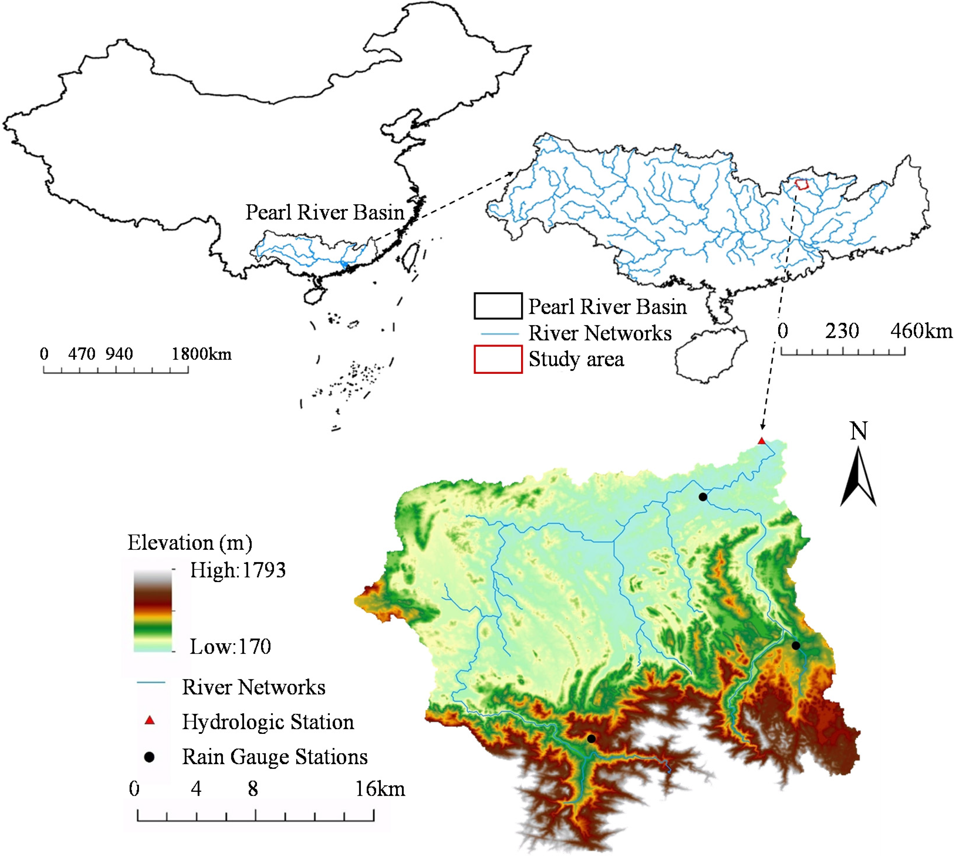
3.1. Study Area

3.2. Data
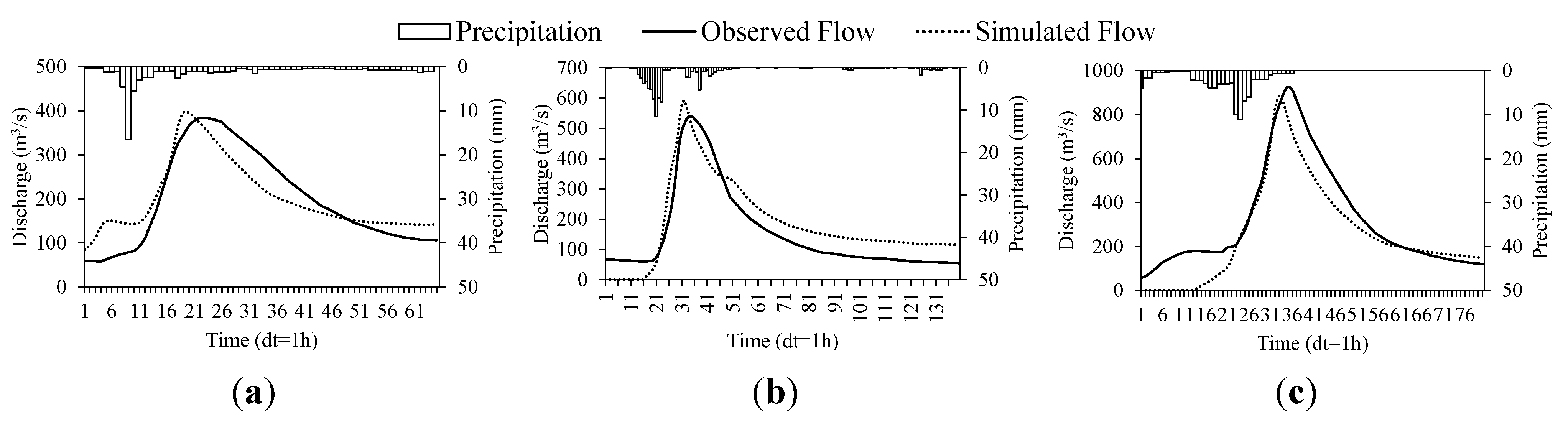
| Event | Magnitude | Precipitation (mm) | Time Step (h) | Duration (h) | Peak Discharge (m3/s) | W0 (mm) | Flood Frequency (%) |
|---|---|---|---|---|---|---|---|
| 198106 | Small | 80.5 | 1 | 131 | 384 | 40 | 75% |
| 198505 | Medium | 90.0 | 1 | 140 | 538 | 50 | 50% |
| 198005 | Large | 99.1 | 1 | 80 | 925 | 60 | 25% |
4. Results and Discussion
4.1. Results of Calibration and Validation
| Period | ENS | WB | EP | ETP (h) |
|---|---|---|---|---|
| Calibration | 0.82 | 1.08 | 0.10 | 0.7 |
| Validation | 0.74 | 1.06 | 0.12 | 1.7 |
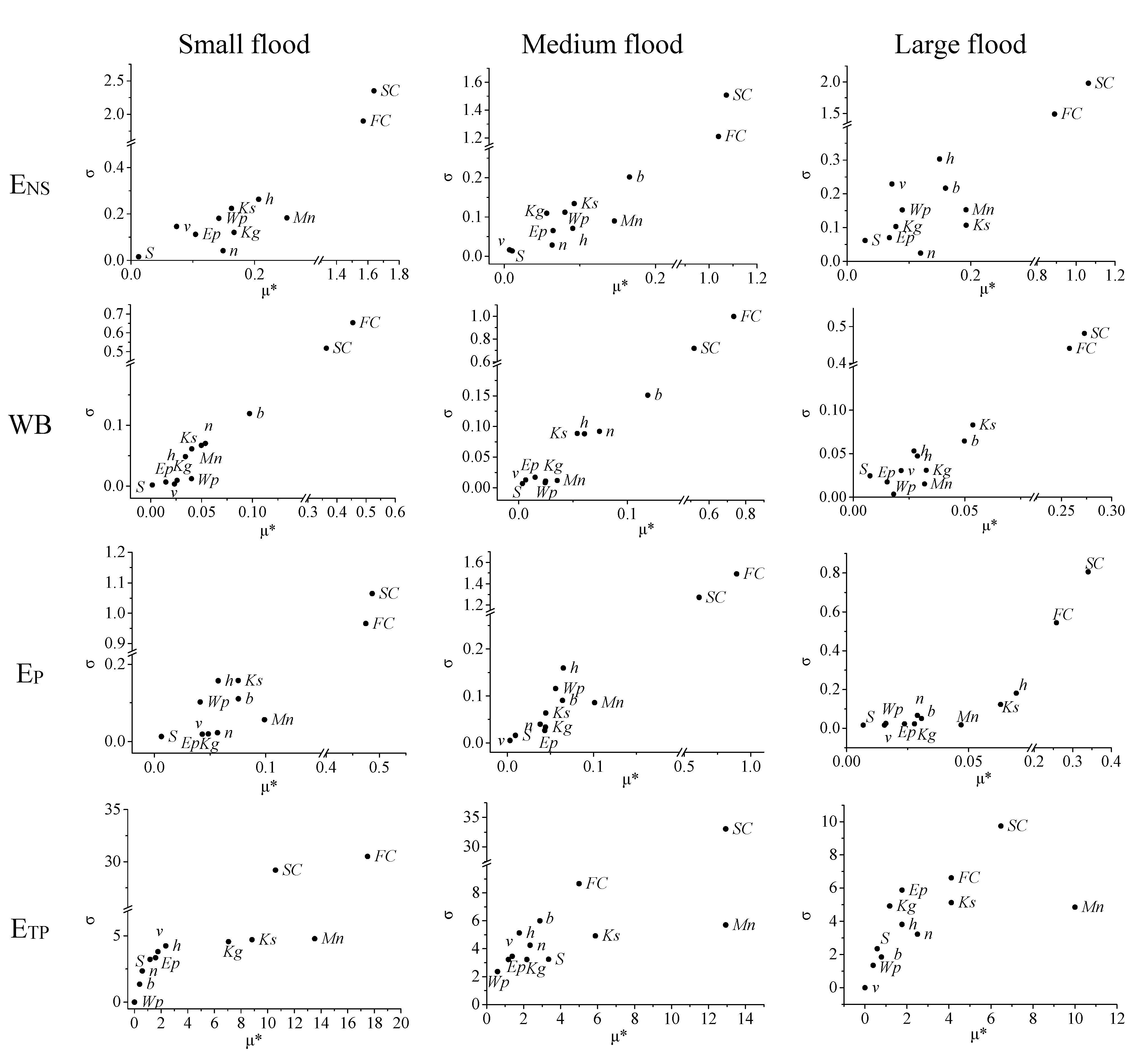
4.2. Results of Morris Screening

4.3. Results of Correlation Identification
| n | Mn | h | b | SC | FC | |
|---|---|---|---|---|---|---|
| Ks | −0.18 | 0.17 | −0.22 * | 0.18 | −0.17 | −0.28 ** |
| n | −0.19 | 0.32 ** | 0.16 | 0.24 * | 0.17 | |
| Mn | −0.34 ** | 0.16 | 0.26 ** | 0.19 | ||
| h | 0.30 ** | −0.19 | −0.16 | |||
| b | 0.16 | 0.24 * | ||||
| SC | 0.96 ** |
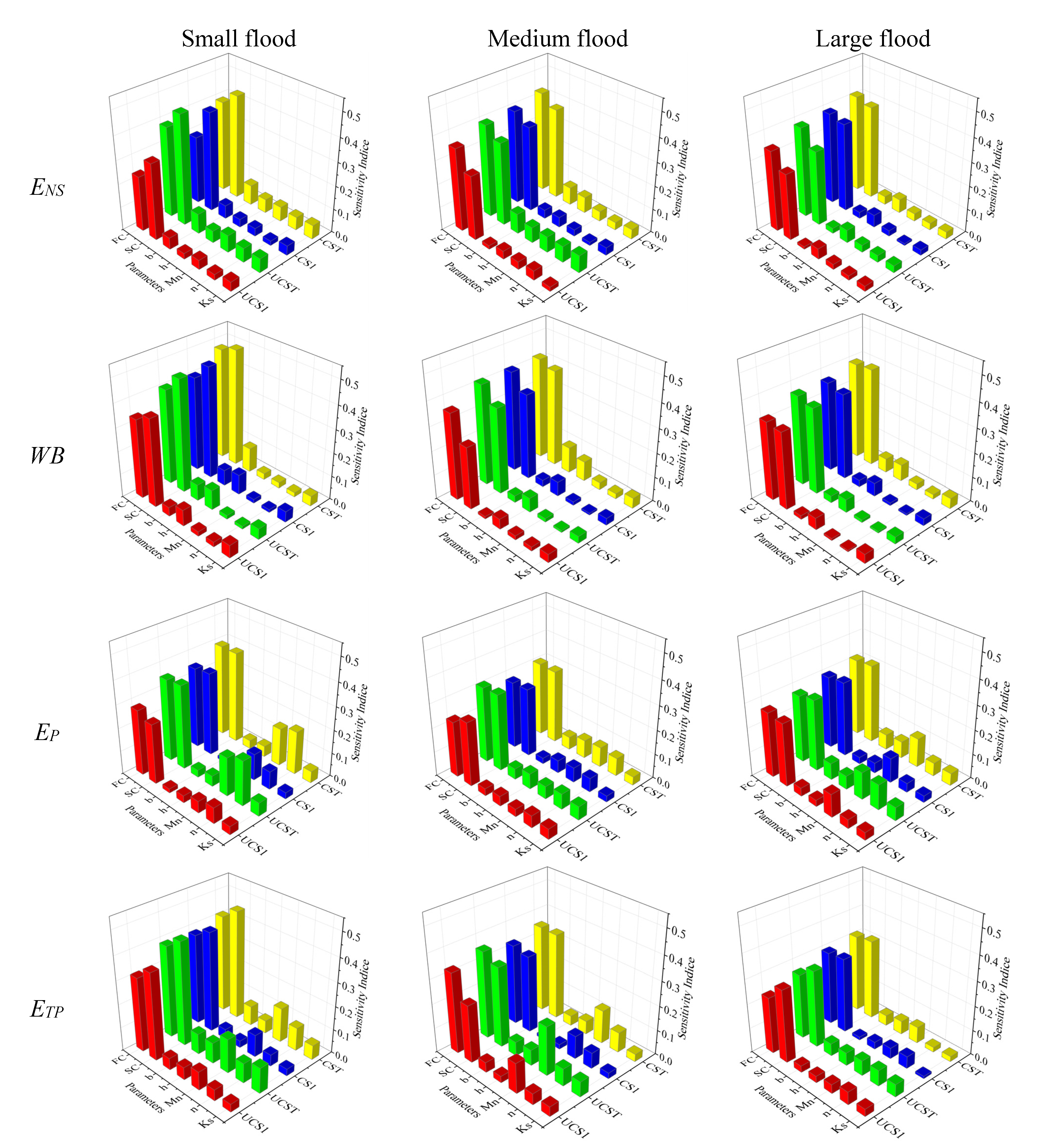
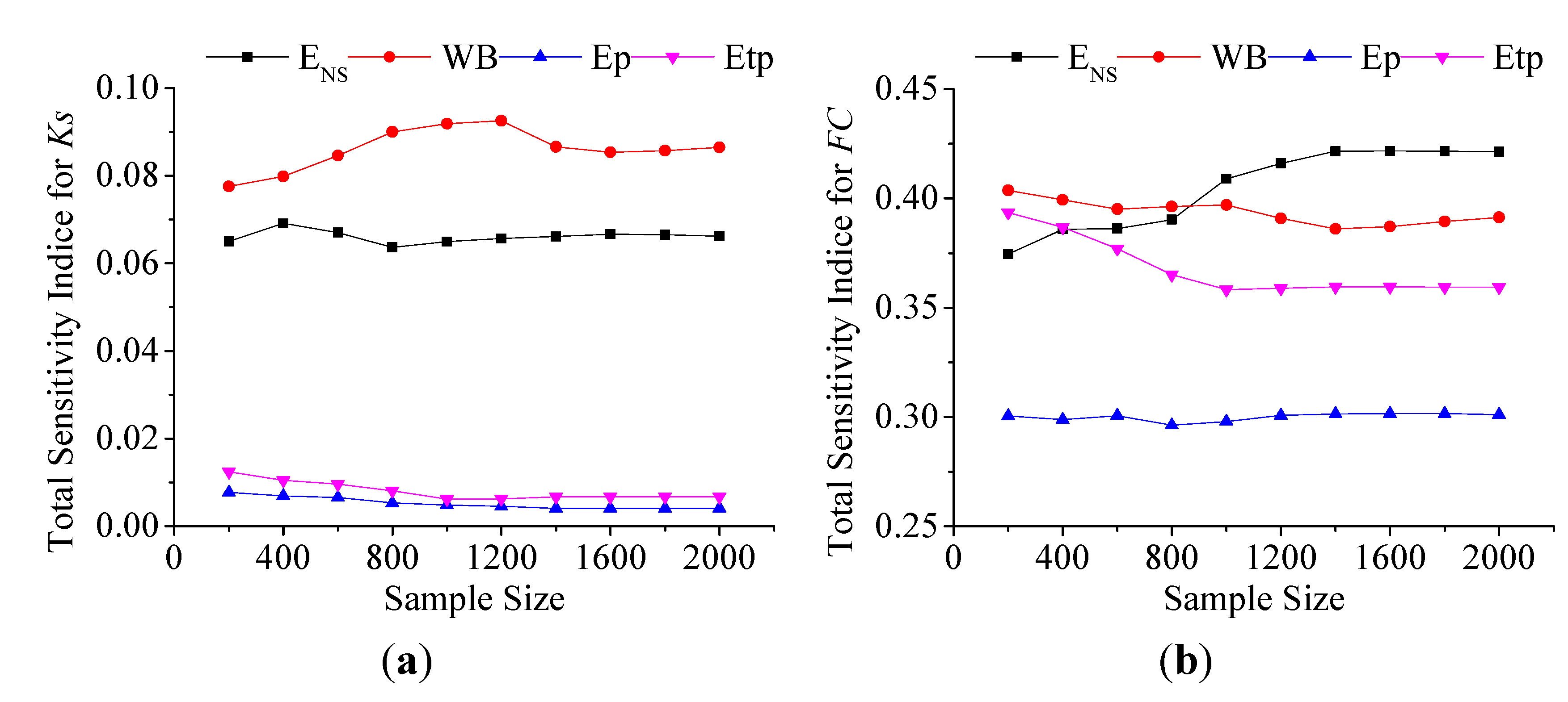
4.4. Results of First and Total Order Sensitivity Analysis

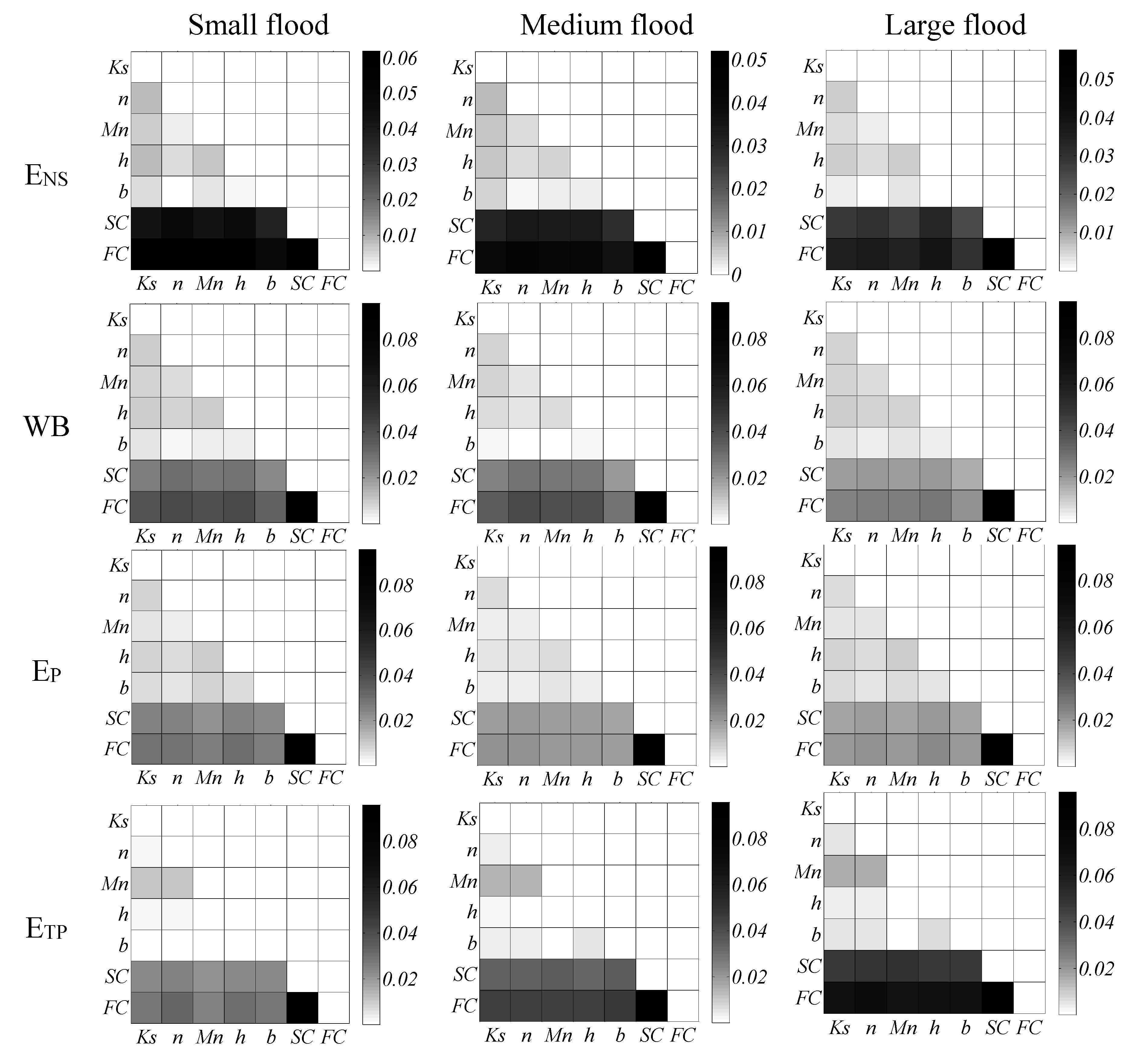
4.5. Results of Second Order and Interactive Sensitivity Analysis
| Objective Functions | First Order | Second Order | Total Order | ||||||
|---|---|---|---|---|---|---|---|---|---|
| Small | Medium | Large | Small | Medium | Large | Small | Medium | Large | |
| ENS | 0.74 | 0.77 | 0.74 | 0.31 | 0.31 | 0.34 | 1.19 | 1.11 | 1.08 |
| WB | 0.82 | 0.74 | 0.75 | 0.24 | 0.23 | 0.28 | 1.06 | 1.00 | 1.09 |
| EP | 0.74 | 0.69 | 0.75 | 0.33 | 0.31 | 0.26 | 1.20 | 1.01 | 1.06 |
| ETP | 0.75 | 0.84 | 0.7 | 0.34 | 0.24 | 0.22 | 1.04 | 1.14 | 1.05 |


5. Conclusions
- The Morris screening method is helpful for computationally demanding distributed models with dozens of parameters. For the 12 parameters in the Liuxihe model, S, v, Wp, Ep, and Kg are detected as insensitive parameters no matter which objective functions or flood magnitudes are selected. The other seven parameters were retained for further global sensitivity analysis.
- The GLUE method provides a convenient approach to identify the correlation relationship between parameters. SC and FC are observed to be nearly linear regressed, with a correlation coefficient of about 0.96 at the significance level of 0.01. Other parameters demonstrated a certain correlated relationship as well.
- For both uncorrelated and correlated parameters, the classification of parameters as first or total order sensitivity indices was affected neither by the choice of objective functions nor by the selection of different flood magnitudes. FC and SC are highly sensitive parameters and the remaining five parameters are sensitive. Meanwhile, the ranking of parameters sensitivity indices was greatly determined by the various objective functions specified and particular flood magnitudes stated. Due to the distinctive antecedent watershed conditions inducing different tolerance to watershed disturbances, the sensitivity indices for small floods were relatively higher than those for large floods. With regard to specific objective functions, flow concentration parameters such as n and Mn had a greater effect on EP and ETP than WB, whereas runoff generation parameters such as Ks, b, and b display totally reversed consequences. Hydrological models behave and respond uniquely to various evaluation functions and application conditions.
- Highly correlated parameters present relatively larger sensitivity indices in the correlated case compared with the uncorrelated, whereas poorly correlated parameters displayed inverse results. Considering that highly sensitive parameters are prone to correlate with each other and commonly sensitive parameters are inclined to be distinguished from other parameters, the sensitivity indices of highly sensitive parameters might be underestimated and that of sensitive parameters might be overestimated without accounting for correlations. Further in-depth second order sensitivity analysis indicated that pairwise interactions, which cannot be neglected, accounted for most interactions.
Acknowledgments
Author Contributions
Conflicts of Interest
References
- Beven, K.J. Rainfall-Runoff Modeling (The Primer), 2nd ed.; John Wiley & Sons, Ltd.: West Sussex, UK, 2012; pp. 1–3. [Google Scholar]
- Wang, G.S.; Xia, J.; Chen, J. Quantification of effects of climate variations and human activities on runoff by a monthly water balance model: A case study of the Chaobai River basin in northern China. Water Resour. Res. 2009, 45. [Google Scholar] [CrossRef] [Green Version]
- Beven, K.; Binley, A. The future of distributed models: Model calibration and uncertainty prediction. Hydrol. Process. 1992, 6, 279–298. [Google Scholar] [CrossRef]
- Beven, K.; Binley, A. GLUE: 20 years on. Hydrol. Process. 2014, 28, 5897–5918. [Google Scholar] [CrossRef]
- Morris, M.D. Factorial sampling plans for preliminary computational experiments. Technometrics 1991, 33, 161–174. [Google Scholar] [CrossRef]
- Zhan, C.; Song, X.; Xia, J.; Tong, C. An efficient approach for global sensitivity analysis of hydrological model parameters. Environ. Model. Softw. 2013, 41, 39–52. [Google Scholar] [CrossRef]
- Van Griensven, A.; Meixner, T.; Grunwald, S.; Bishop, T.; Diluzio, M.; Srinivasan, R.A. Global sensitivity analysis tool for the parameters of multi-variable catchment models. J. Hydrol. 2006, 324, 10–23. [Google Scholar] [CrossRef]
- Katz, R.W. Extreme value theory for precipitation: Sensitivity analysis for climate change. Adv. Water. Resour. 1999, 23, 133–139. [Google Scholar] [CrossRef]
- Plischke, E.; Borgonovo, E.; Smith, C.L. Global sensitivity measures from given data. Eur. J. Oper. Res. 2013, 226, 536–550. [Google Scholar] [CrossRef]
- Jung, Y.; Merwade, V.; Kim, S.; Kang, N.; Kim, Y.; Lee, K.; Kim, G.; Kim, H.S. Sensitivity of subjective decisions in the GLUE methodology for quantifying the uncertainty in the flood inundation map for Seymour reach in Indiana, USA. Water 2014, 6, 2014–2126. [Google Scholar] [CrossRef]
- Doherty, J.; Welter, D. A short exploration of structural noise. Water Resour. Res. 2010, 46. [Google Scholar] [CrossRef]
- Foglia, L.; Hill, M.C.; Mehl, S.W.; Burlando, P. Evaluating model structure adequacy: The case of the Maggia Valley groundwater system, Southern Switzerland. Water Resour. Res. 2013, 49. [Google Scholar] [CrossRef]
- Rakovec, O.; Hill, M.C.; Clark, M.P.; Weerts, A.H.; Teuling, A.J.; Uijlenhoet, R. Distributed evaluation of local sensitivity analysis (DELSA), with application to hydrologic models. Water Resour. Res. 2014, 50. [Google Scholar] [CrossRef]
- Tang, Y.; Reed, P.; Wagener, T.; van Werkhoven, K. Comparing sensitivity analysis methods to advance lumped watershed model identification and evaluation. Hydrol. Earth Syst. Sci. 2007, 11, 793–817. [Google Scholar] [CrossRef]
- Gan, Y.; Duan, Q.; Gong, W.; Tong, C.; Sun, Y.; Chu, W.; Ye, A.; Miao, C.; Di, Z. A comprehensive evaluation of various sensitivity analysis methods: A case study with a hydrological model. Environ. Model. Softw. 2014, 51, 269–285. [Google Scholar] [CrossRef]
- Cibin, R.; Sudheer, K.P.; Chaubey, I. Sensitivity and identifiability of stream flow generation parameters of the SWAT model. Hydrol. Process. 2010, 24, 1133–1148. [Google Scholar] [CrossRef]
- Hornberger, G.; Spear, R. An approach to the preliminary analysis of environmental systems. J. Environ. Manag. 1981, 12, 7–18. [Google Scholar]
- Doherty, J.; Johnston, V.K. Methodologies for calibration and predictive analysis of a watershed model. J. Am. Water. Resour. Assoc. 2003, 39, 251–265. [Google Scholar] [CrossRef]
- Mokhtari, A.; Frey, H.C. Sensitivity analysis of a two-dimensional probabilistic risk assessment model using analysis of variance. Risk Anal. 2005, 25, 1511–1529. [Google Scholar] [CrossRef] [PubMed]
- Reusser, D.E.; Buytaert, W.; Zehe, E. Temporal dynamics of model parameter sensitivity for computationally expensive models with the Fourier amplitude sensitivity test. Water Resour. Res. 2011, 47. [Google Scholar] [CrossRef]
- Zhang, X.L.; Peng, Y.; Xu, W.; Wang, B.D.; Wang, H.X. Sensitivity analysis of Xinanjiang model prameters using Sobol’ method. South-North Water Trans. Water Sci. Technol. 2014, 12, 27–32. (In Chinese) [Google Scholar]
- Sobol’, I.M. Sensitivity estimates for nonlinear mathematical models. Math. Model. Comput. Exp. 1993, 1, 407–417. [Google Scholar]
- Zhang, C.; Chu, J.; Fu, G. Sobol’s sensitivity analysis for a distributed hydrological model of Yichun River Basin, China. J. Hydrol. 2013, 480, 58–68. [Google Scholar] [CrossRef]
- Wagener, T.; van Werkhoven, K.; Reed, P.M.; Tang, Y. Multiobjective sensitivity analysis to understand the information content in streamflow observation for distributed watershed modeling. Water Resour. Res. 2009, 45. [Google Scholar] [CrossRef]
- Nossent, J.; Elsen, P.; Bauwens, W. Sobol’ sensitivity analysis of a complex environmental method. Environ. Model. Softw. 2011, 26, 1515–1525. [Google Scholar] [CrossRef]
- Zhan, Y.; Zhang, M. Application of a combined sensitivity analysis approach on a pesticide environmental risk indicator. Environ. Model. Softw. 2013, 49, 129–140. [Google Scholar] [CrossRef]
- Todri, E.; Amenaghawon, A.N.; del Val, I.J.; Leak, D.J.; Kontoravdi, C.; Sergei Kucherenko, S.; Nilay Shah, N. Global sensitivity analysis and meta-modeling of an ethanol production process. Chem. Eng. Sci. 2014, 114, 114–127. [Google Scholar] [CrossRef]
- Liu, K.; Zeng, X.; Qiao, L.; Li, X.; Yang, Y.; Dai, C.; Hou, A.; Xu, D. The sensitivity and significance analysis of parameters in the model of ph regulation on lactic acid production by Lactobacillus bulgaricus. BMC Bioinform. 2014, 15. [Google Scholar] [CrossRef] [PubMed]
- Lagerwalla, G.; Kiker, G.; Muñoz-Carpena, R.; Wang, N. Global uncertainty and sensitivity analysis of a spatially distributed ecological model. Ecol. Model. 2014, 275, 22–30. [Google Scholar] [CrossRef]
- Kucherenko, S.; Tarantola, S.; Annoni, P. Estimation of global sensitivity indices for models with dependent variables. Comput. Phys. Commun. 2012, 183, 937–946. [Google Scholar] [CrossRef]
- Saltelli, A. Making best use of model evaluations to compute sensitivity indices. Comput. Phys. Commun. 2002, 145, 280–297. [Google Scholar] [CrossRef]
- Campolongo, F.; Saltelli, A.; Cariboni, J. From screening to quantitative sensitivity analysis: A unified approach. Comput. Phys. Commun. 2011, 182, 978–988. [Google Scholar] [CrossRef]
- Sweetapple, C.; Fu, G.; Butler, D. Identifying key sources of uncertainty in the modelling of greenhouse gas emission from wastewater treatment. Water Res. 2013, 47, 4652–4665. [Google Scholar] [CrossRef] [PubMed]
- Sweetapple, C.; Fu, G.; Butler, D. Identifying sensitive sources and key operational parameters for the reduction of greenhouse gas emissions from wastewater treatment. Water Res. 2014, 62, 249–259. [Google Scholar] [CrossRef] [PubMed] [Green Version]
- Campolongo, F.; Cariboni, J.; Saltelli, A. An effective screening design for sensitivity analysis of large models. Environ. Model. Softw. 2007, 22, 1509–1518. [Google Scholar] [CrossRef]
- McKay, M.D.; Beckman, R.J.; Conover, W.J. A comparison of three methods for selecting values of input variables in the analysis of output from a computer code. Technometrics 1979, 21, 239–245. [Google Scholar] [CrossRef]
- Andres, T.H. Sampling method and sensitivity analysis for large parameter sets. J. Stat. Comput. Simul. 1997, 57, 77–110. [Google Scholar] [CrossRef]
- Ratto, M.; Tarantola, S.; Saltelli, A. Sensitivity analysis in model calibration: GSA-GLUW approach. Comput. Phys. Commun. 2001, 136, 212–224. [Google Scholar] [CrossRef]
- Zhao, S.; Zhang, W.; Lin, X.; Li, J.; Song, D.; He, X. Effect of parameters correlation on uncertainty and sensitivity in dynamic thermal analysis of thermal protection blanket in service. Int. J. Therm. Sci. 2015, 87, 158–168. [Google Scholar] [CrossRef]
- Chen, Y.B.; Ren, Q.W.; Huang, F.H.; Xu, H.; Cluckie, L. Liuxihe model and its modeling to river basin flood. J. Hydrol. Eng. 2011, 16, 33–50. [Google Scholar] [CrossRef]
- Chen, Y.; Huang, F.; Xu, H. Research on flood forecasting of the Lianjiang River Basin based on physically based distributed hydrological model. In Proceedings of the Academic Annual Conference of Chinese Hydraulic Engineering Society, Haikou, China, 1–4 April 2008; pp. 955–960. (In Chinese)
- Huang, S.; Chen, Y.; Jiang, H. Flood forecasting of the Wu River Basin based on the Liuxihe model. In Proceedings of the 4th Youth Science and Technology Forum of the Annual Conference of Chinese Hydraulic Engineering Society, Beijing, China, 15 October 2008; pp. 255–260. (In Chinese)
- Fan, Z.; Hao, Z.; Chen, Y.; Wang, J.; Huang, F. The application and research of income flood simulation of the Baipengzhu Reservior with the Liuxihe Model. Acta Sci. Nat. Univ. SunYatSeni 2012, 51, 113–118. (In Chinese) [Google Scholar]
- Liao, H.; Chen, Y.; Xu, H.; He, J. Study of Liuxihe model for flood and rainfall forecast of Tiantoushui watershed. Yangtze River 2012, 43, 12–16. (In Chinese) [Google Scholar]
- Campbell, G.S. A simple method for determining unsaturated conductivity from moisture retention data. Soil Sci. 1974, 117, 311–314. [Google Scholar] [CrossRef]
- Freer, J.; Beven, K.J.; Ambroise, B. Bayesian estimation of uncertainty in runoff prediction and the value of data: An application of the GLUE approach. Water Resour. Res. 1996, 32, 2162–2173. [Google Scholar] [CrossRef]
- Manache, G.; Melching, C.S. Identification of reliable regression- and correlation-based sensitivity measures for importance ranking of water-quality model parameters. Environ. Model. Softw. 2008, 23, 549–562. [Google Scholar] [CrossRef]
- Tong, C.; Graziani, F. A practical global sensitivity analysis methodology for multi-physics applications. Lect. Notes Comput. Sci. Eng. 2008, 62, 277–299. [Google Scholar]
- Arya, L.M.; Paris, J.F. A physioempirical model to predict the soil moisture characteristic from particle-size distribution and bulk density data. Soil Sci. Soc. Am. J. 1981, 45, 1023–1030. [Google Scholar] [CrossRef]
- Nash, J.E.; Sutcliffe, J. River flow forecasting through conceptual models. Part 1. A discussion of principles. J. Hydrol. 1970, 10, 282–290. [Google Scholar] [CrossRef]
- Kannan, N.; White, S.M.; Worrall, F.; Whelan, M.J. Sensitivity analysis and identification of the best evapotranspiration and runoff options for hydrological modelling in SWAT-2000. J. Hydrol. 2007, 332, 456–466. [Google Scholar] [CrossRef]
- Van Werkhoven, K.; Wagener, T.; Reed, P.; Tang, Y. Sensitivity-guided reduction of parametric dimensionality for multi-objective calibration of watershed models. Adv. Water Resour. 2009, 32, 1154–1169. [Google Scholar] [CrossRef]
- Dobler, C.; Pappenberger, F. Global sensitivity analyses for a complex hydrological model applied in an Alpine watershed. Hydrol. Process. 2013, 27, 3922–3940. [Google Scholar] [CrossRef]
- Xu, H.; Chen, Y.; Li, Z.; He, J. Analysis on parameter sensitivity of distributed hydrological model based on LH-OAT Method. Yangtze River 2012, 43, 19–23. (In Chinese) [Google Scholar]
- Pan, F.; Zhu, J.; Ye, M.; Pachepsky, Y.A.; Wu, Y.S. Sensitivity analysis of unsaturated flow and contaminant transport with correlated parameters. J. Hydrol. 2011, 397, 238–249. [Google Scholar] [CrossRef]
- Massmann, C.; Holzmann, H. Analysis of the behavior of a rainfall-runoff model using three global sensitivity analysis methods evaluated at different temporal scales. J. Hydrol. 2012, 475, 97–110. [Google Scholar] [CrossRef]
- Baroni, G.; Tarantola, S. A General Probabilistic Framework for uncertainty and global sensitivity analysis of deterministic models: A hydrological case study. Environ. Model. Softw. 2014, 51, 26–34. [Google Scholar] [CrossRef]
© 2015 by the authors; licensee MDPI, Basel, Switzerland. This article is an open access article distributed under the terms and conditions of the Creative Commons Attribution license (http://creativecommons.org/licenses/by/4.0/).
Share and Cite
Wan, H.; Xia, J.; Zhang, L.; She, D.; Xiao, Y.; Zou, L. Sensitivity and Interaction Analysis Based on Sobol’ Method and Its Application in a Distributed Flood Forecasting Model. Water 2015, 7, 2924-2951. https://doi.org/10.3390/w7062924
Wan H, Xia J, Zhang L, She D, Xiao Y, Zou L. Sensitivity and Interaction Analysis Based on Sobol’ Method and Its Application in a Distributed Flood Forecasting Model. Water. 2015; 7(6):2924-2951. https://doi.org/10.3390/w7062924
Chicago/Turabian StyleWan, Hui, Jun Xia, Liping Zhang, Dunxian She, Yang Xiao, and Lei Zou. 2015. "Sensitivity and Interaction Analysis Based on Sobol’ Method and Its Application in a Distributed Flood Forecasting Model" Water 7, no. 6: 2924-2951. https://doi.org/10.3390/w7062924