
Spatial Downscaling of TRMM Precipitation Product Using a Combined Multifractal and Regression Approach: Demonstration for South China


Abstract
:1. Introduction
2. Materials and Methods
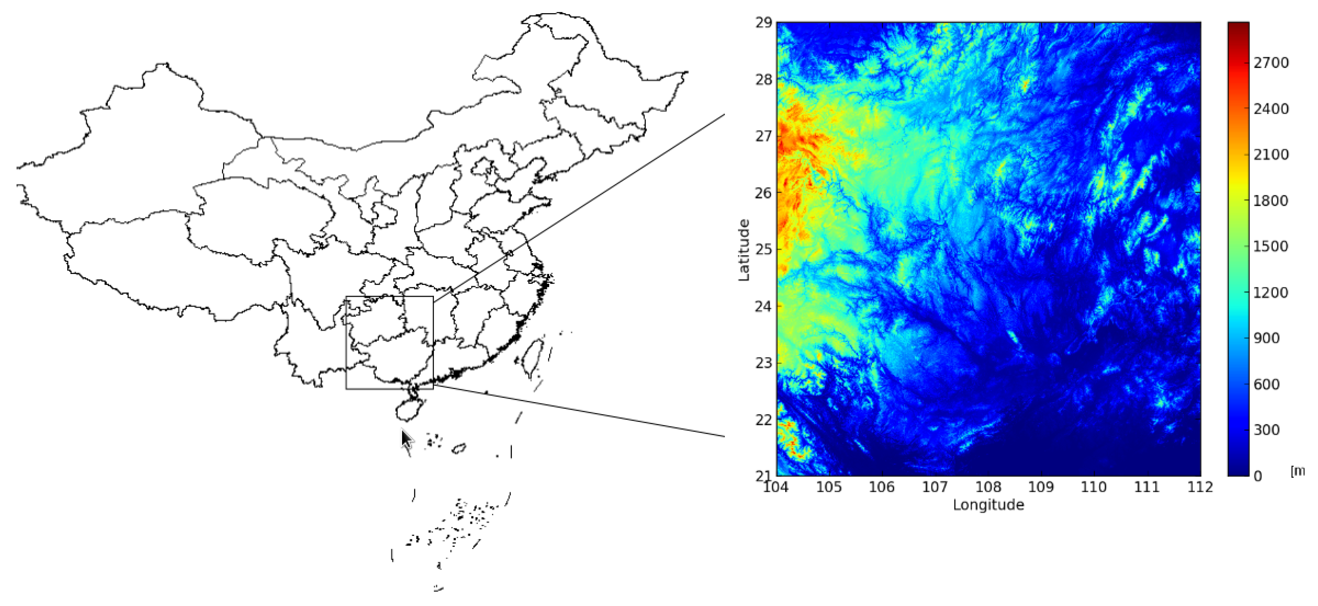
2.1. Study Area

2.2. Datasets
2.2.1. Tropical Rainfall Measuring Mission (TRMM) Precipitation Data
2.2.2. DEM Data
2.2.3. Station Precipitation Data
2.3. Methods
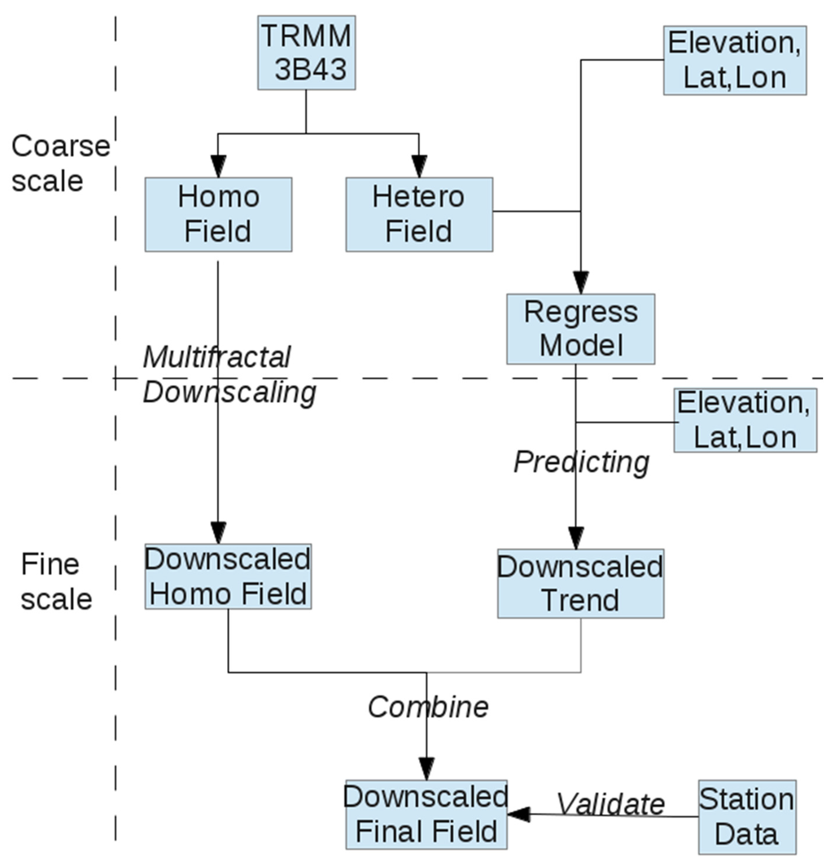
2.3.1. Downscaling

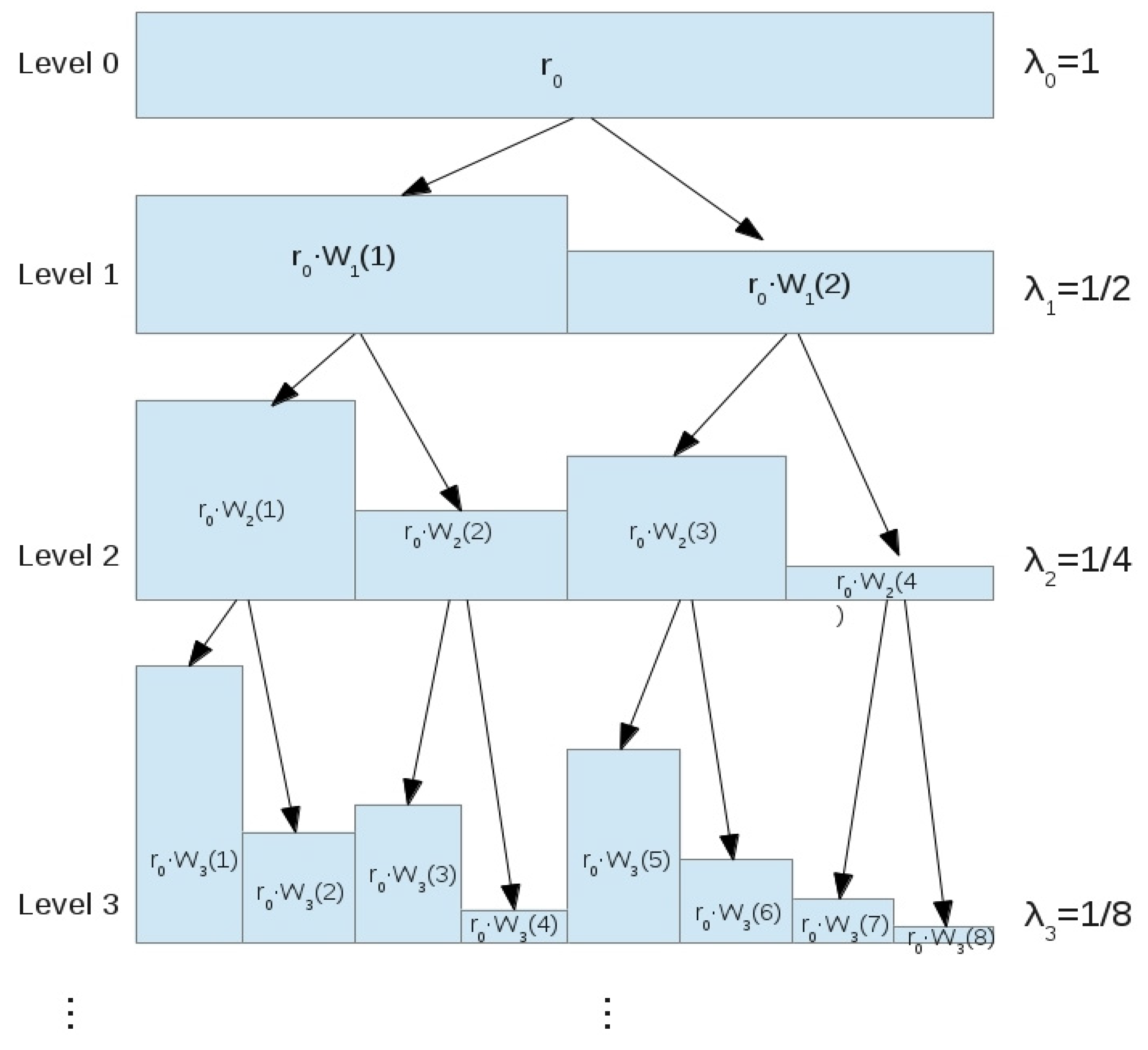
2.3.2. Multifractal Model
2.3.3. Regression Model
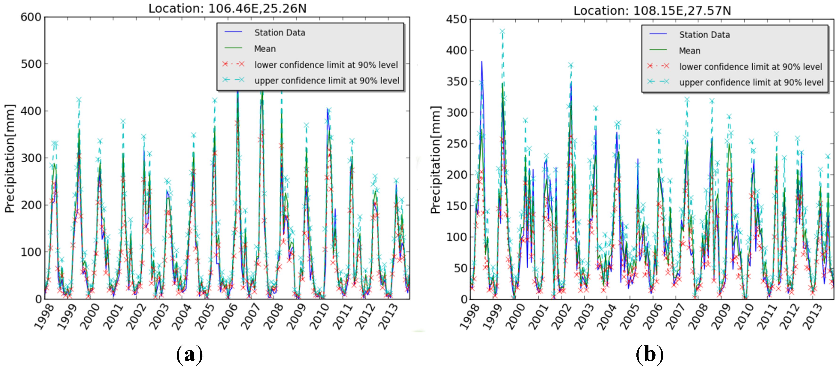
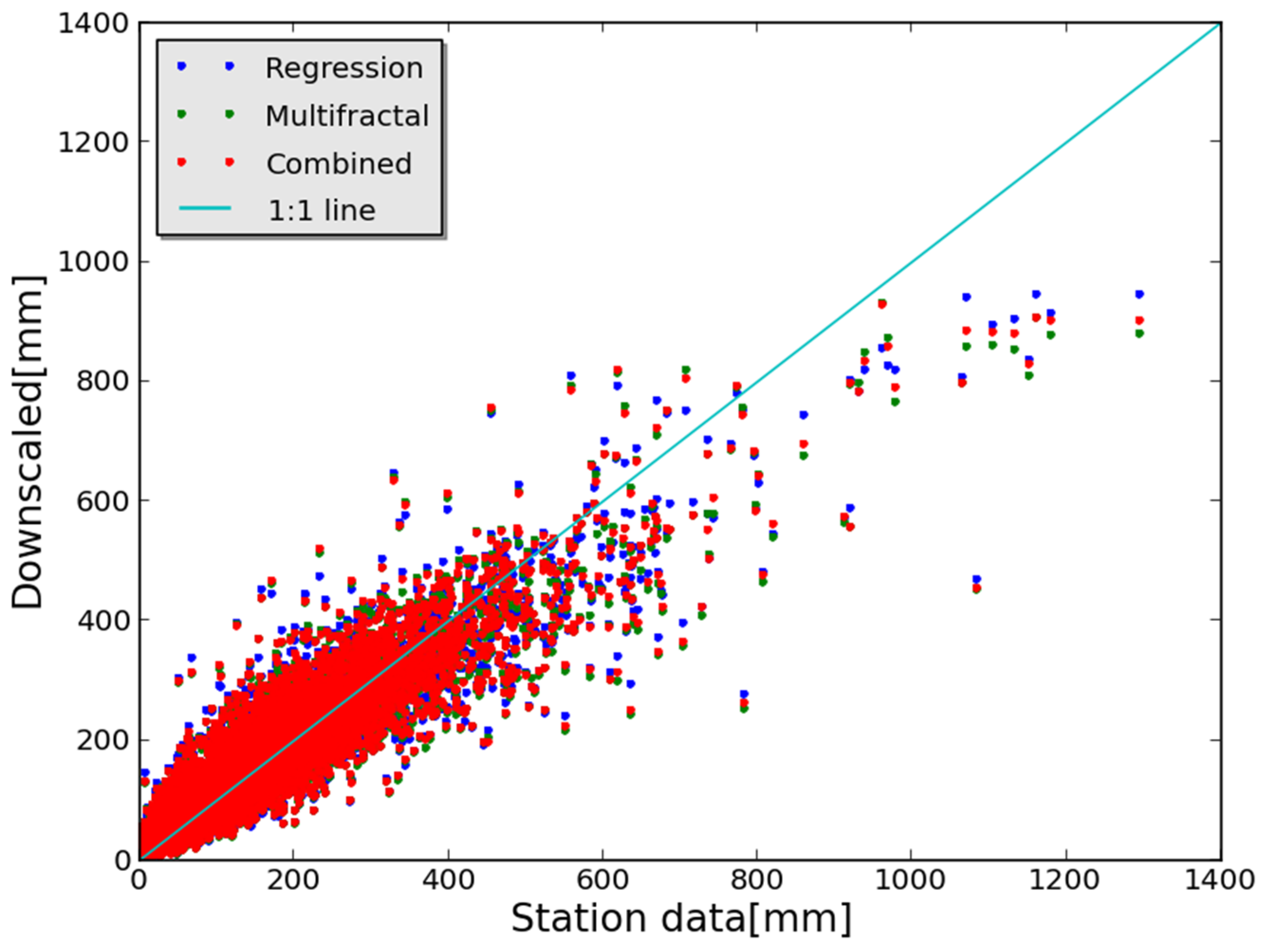
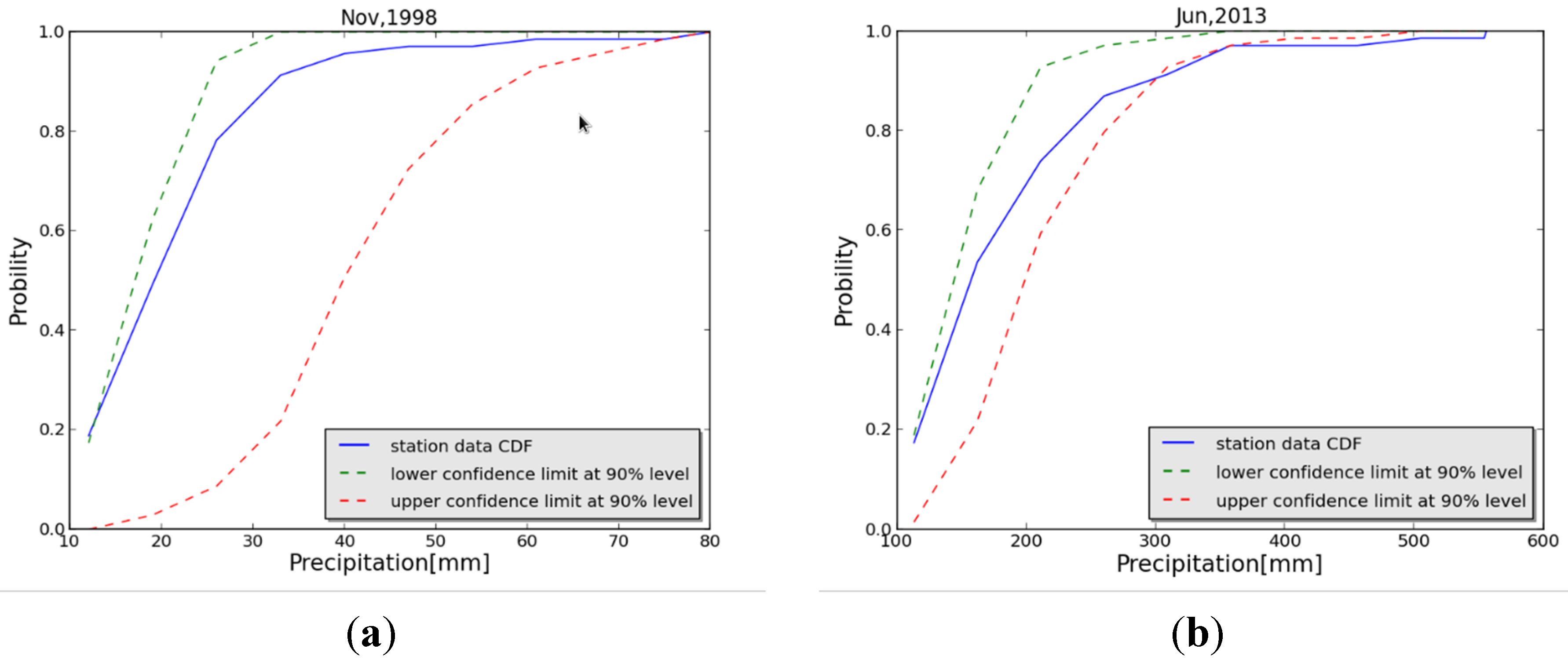
2.3.4. Validation
3. Results
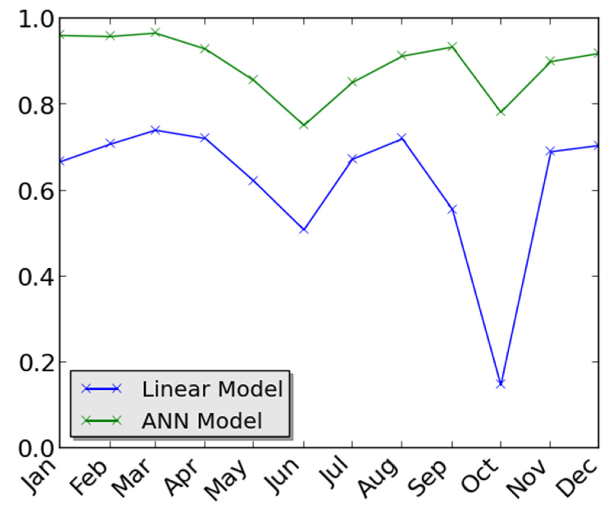
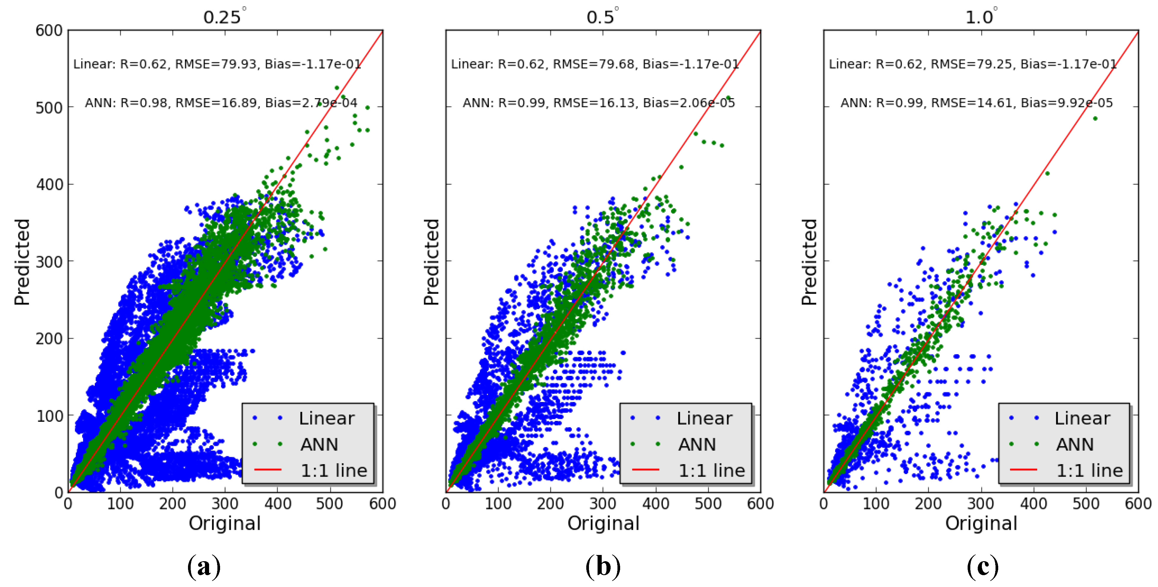
3.1. Regression Analysis


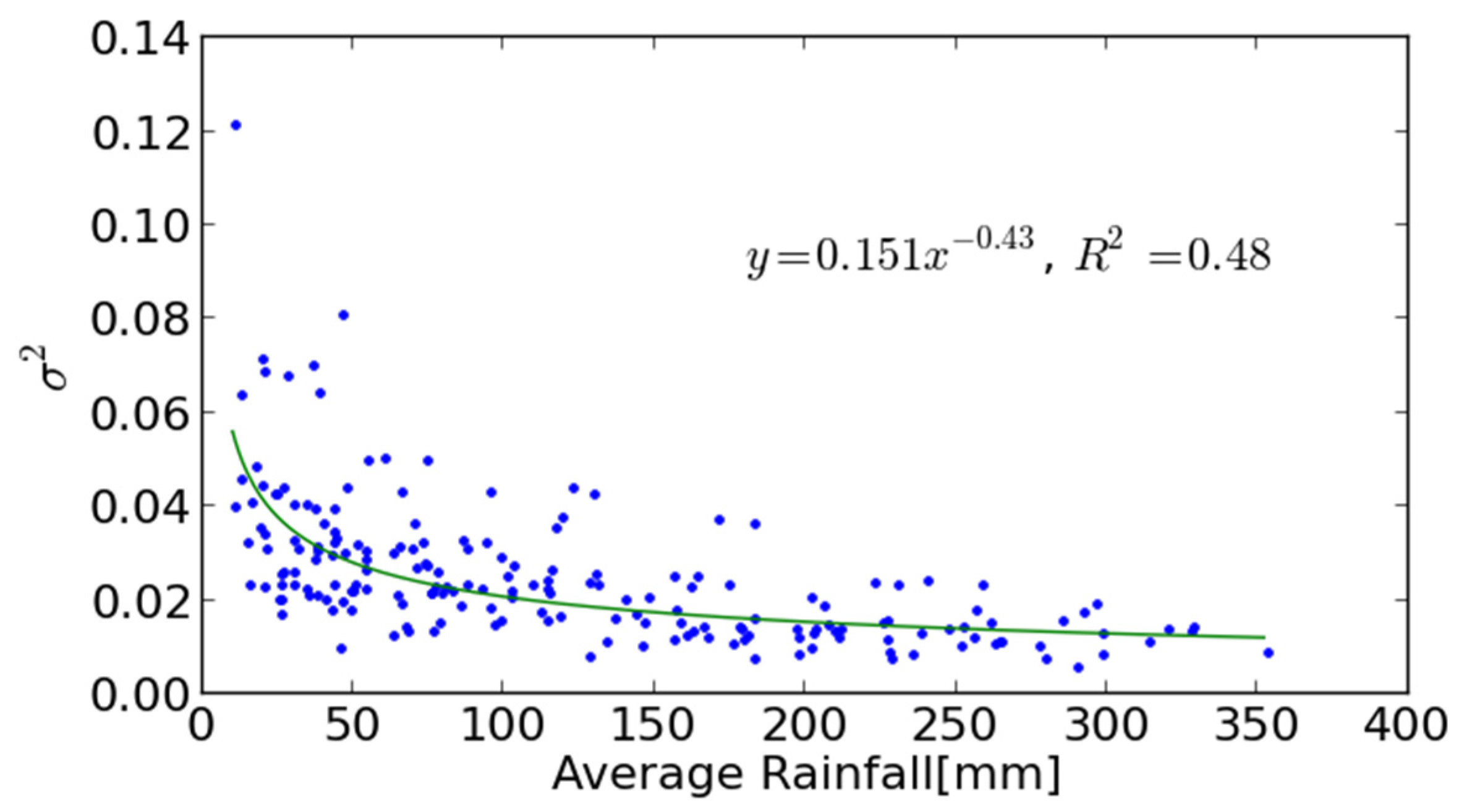
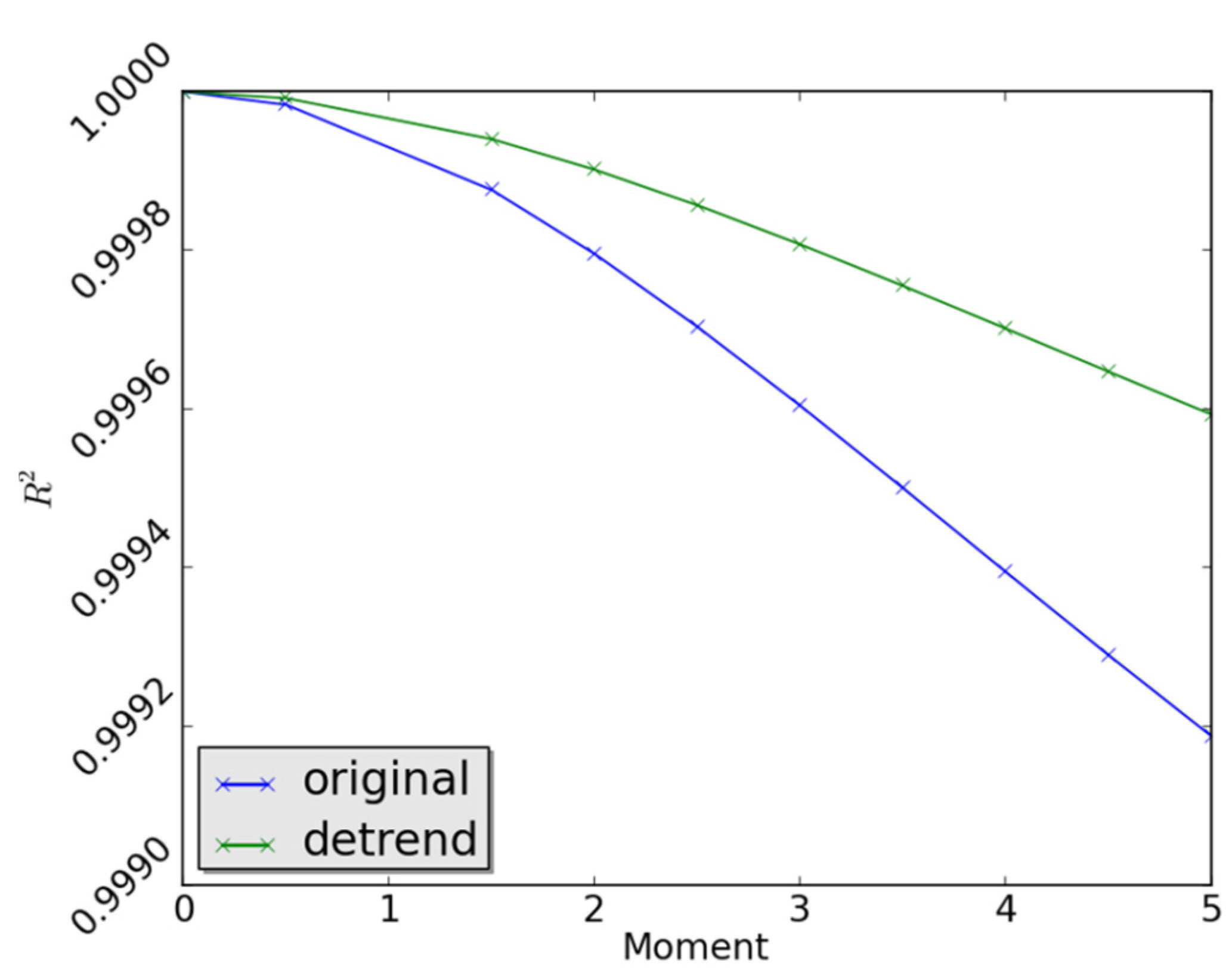
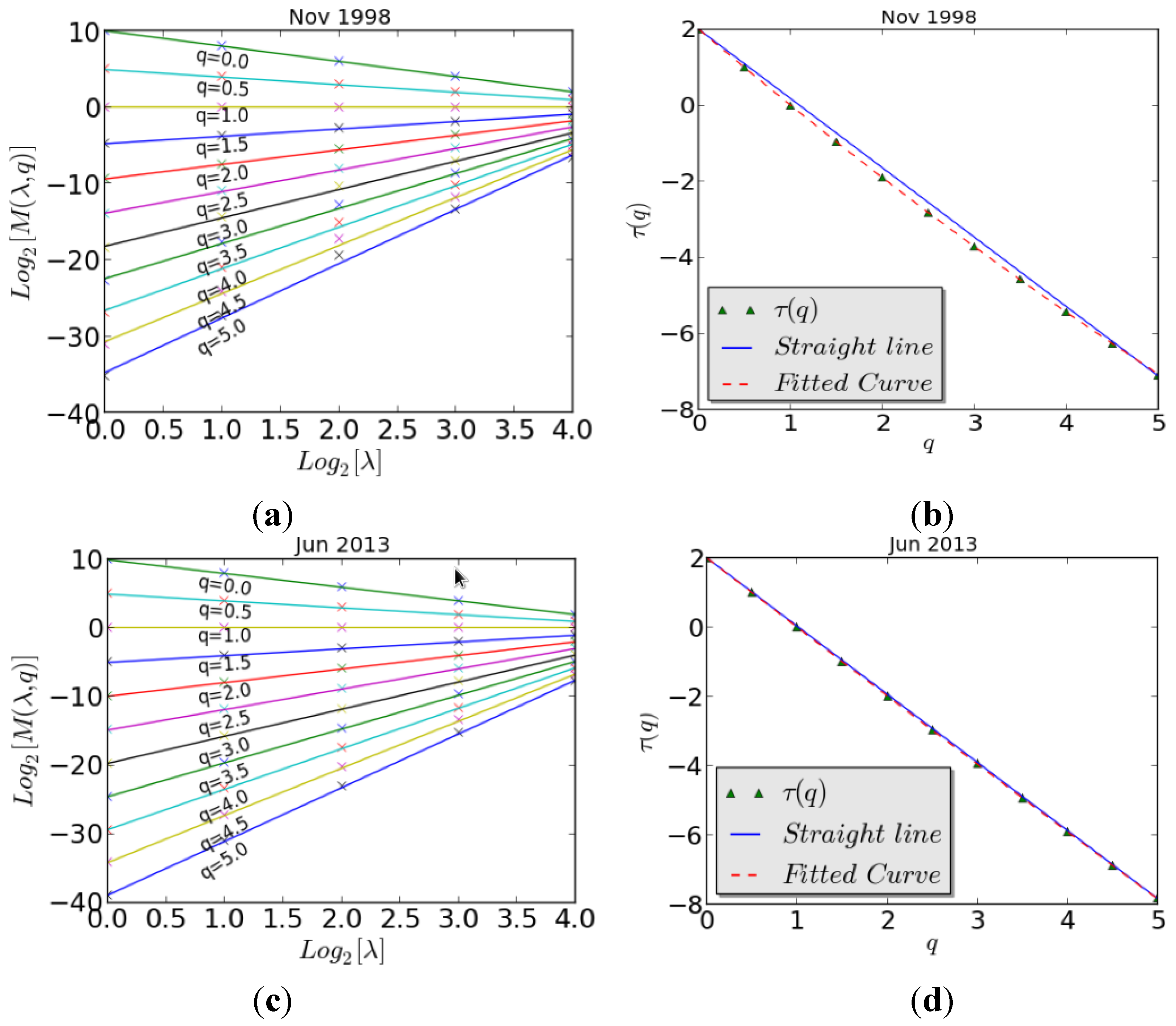
3.2. Multifractal Analysis


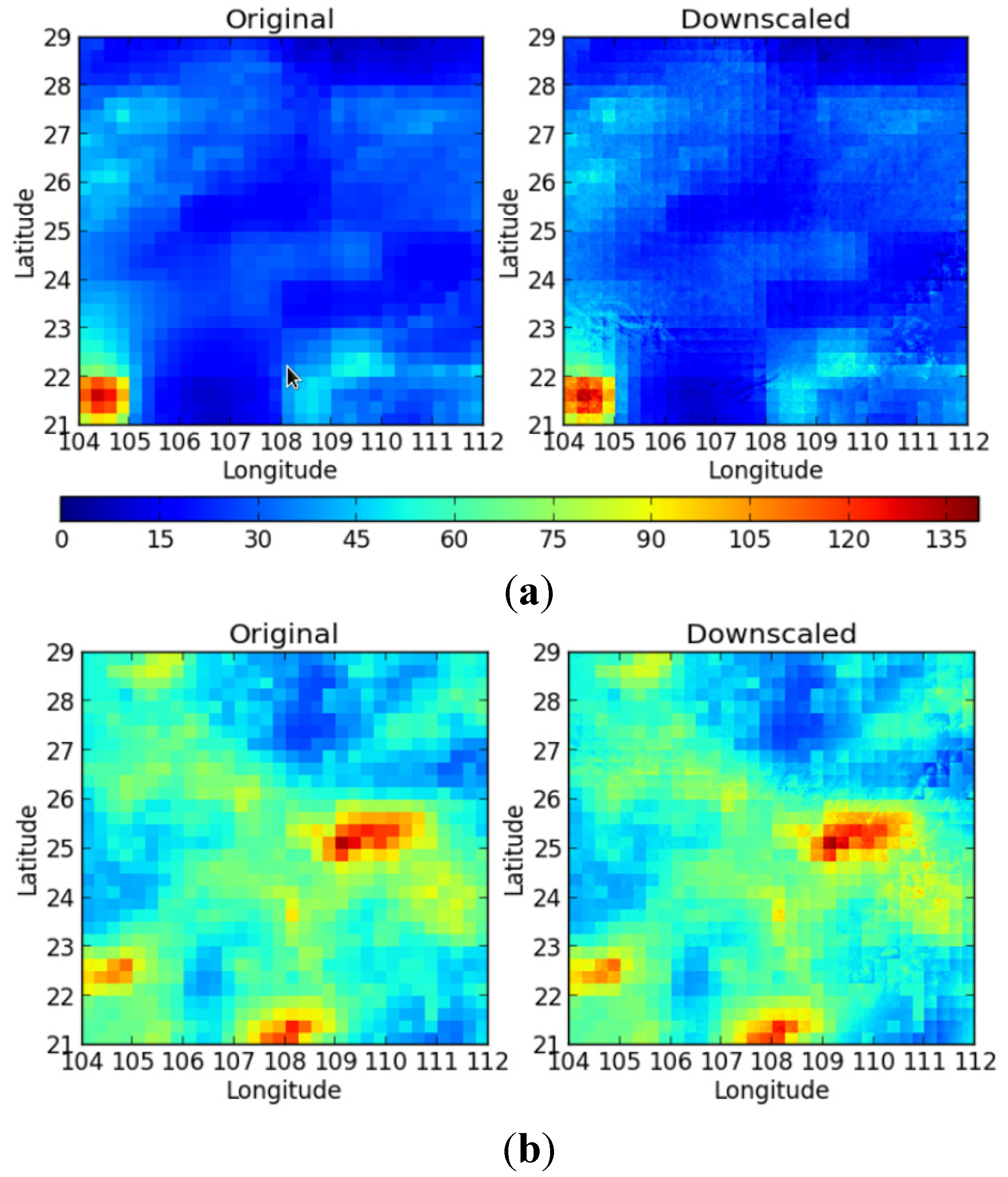
3.3. Downscaling


| Index | ANN | MF | Combined |
|---|---|---|---|
| R | 0.936 | 0.934 | 0.935 |
| RMSE | 40.56 | 41.20 | 41.04 |
| Bias | 0.042 | 0.037 | 0.041 |

4. Discussion
5. Conclusions
Acknowledgments
Author Contributions
Conflicts of Interest
References
- Goovaerts, P. Geostatistical approaches for incorporating elevation into the spatial interpolation of rainfall. J. Hydrol. 2000, 228, 113–129. [Google Scholar] [CrossRef]
- Jia, S.F.; Zhu, W.B.; Lu, A.F.; Yan, T.T. A statistical spatial downscaling algorithm of trmm precipitation based on ndvi and dem in the qaidam basin of china. Remote Sens. Environ. 2011, 115, 3069–3079. [Google Scholar] [CrossRef]
- Kyriakidis, P.C.; Kim, J.; Miller, N.L. Geostatistical mapping of precipitation from rain gauge data using atmospheric and terrain characteristics. J. Appl. Meteorol. 2001, 40, 1855–1877. [Google Scholar] [CrossRef]
- Langella, G.; Basile, A.; Bonfante, A.; Terribile, F. High-Resolution space-time rainfall analysis using integrated ann inference systems. J. Hydrol. 2010, 387, 328–342. [Google Scholar] [CrossRef]
- Li, M.; Shao, Q.X. An improved statistical approach to merge satellite rainfall estimates and raingauge data. J. Hydrol. 2010, 385, 51–64. [Google Scholar] [CrossRef]
- Badas, M.G.; Deidda, R.; Piga, E. Modulation of homogeneous space-time rainfall cascades to account for orographic influences. Nat. Hazards Earth Syst. Sci. 2006, 6, 427–437. [Google Scholar] [CrossRef]
- Goodrich, D.C.; Simanton, J.R. Water research and management in semiarid environments. J. Soil Water Conserv. 1995, 50, 416–419. [Google Scholar]
- Hu, Q.F.; Yang, D.W.; Wang, Y.T.; Yang, H.B. Accuracy and spatio-temporal variation of high resolution satellite rainfall estimate over the ganjiang river basin. Sci. China Technol. Sci. 2013, 56, 853–865. [Google Scholar] [CrossRef]
- Xie, P.P.; Arkin, P.A. Analyses of global monthly precipitation using gauge observations, satellite estimates, and numerical model predictions. J. Clim. 1996, 9, 840–858. [Google Scholar] [CrossRef]
- Wilheit, T.T. Some comments on passive microwave measurement of rain. Bull. Am. Meteorol. Soc. 1986, 67, 1226–1236. [Google Scholar] [CrossRef]
- Kummerow, C.; Barnes, W.; Kozu, T.; Shiue, J.; Simpson, J. The tropical rainfall measuring mission (trmm) sensor package. J. Atmos. Ocean. Technol. 1998, 15, 809–817. [Google Scholar] [CrossRef]
- Islam, M.N.; Uyeda, H. Use of trmm in determining the climatic characteristics of rainfall over bangladesh. Remote Sens. Environ. 2007, 108, 264–276. [Google Scholar] [CrossRef]
- Karaseva, M.O.; Prakash, S.; Gairola, R.M. Validation of high-resolution trmm-3b43 precipitation product using rain gauge measurements over kyrgyzstan. Theor. Appl. Climatol. 2012, 108, 147–157. [Google Scholar] [CrossRef]
- Park, N.W. Spatial downscaling of trmm precipitation using geostatistics and fine scale environmental variables. Adv. Meteorol. 2013. [Google Scholar] [CrossRef]
- Schuurmans, J.M.; Bierkens, M.F.P. Effect of spatial distribution of daily rainfall on interior catchment response of a distributed hydrological model. Hydrol. Earth Syst. Sci. 2007, 11, 677–693. [Google Scholar] [CrossRef]
- Guo, J.Z.; Liang, X.; Leung, L.R. Impacts of different precipitation data sources on water budgets. J. Hydrol. 2004, 298, 311–334. [Google Scholar] [CrossRef]
- Smith, M.B.; Koren, V.I.; Zhang, Z.; Reed, S.M.; Pan, J.J.; Moreda, F. Runoff response to spatial variability in precipitation: An analysis of observed data. J. Hydrol. 2004, 298, 267–286. [Google Scholar] [CrossRef]
- Immerzeel, W.W.; Rutten, M.M.; Droogers, P. Spatial downscaling of trmm precipitation using vegetative response on the iberian peninsula. Remote Sens. Environ. 2009, 113, 362–370. [Google Scholar] [CrossRef]
- Fang, J.; Du, J.; Xu, W.; Shi, P.J.; Li, M.; Ming, X.D. Spatial downscaling of trmm precipitation data based on the orographical effect and meteorological conditions in a mountainous area. Adv. Water Resour. 2013, 61, 42–50. [Google Scholar] [CrossRef]
- Evertsz, C.J.G.; Mandelbrot, B.B. Harmonic measure around a linearly self-similar tree. J. Phys. A Math. Gen. 1992, 25, 1781–1797. [Google Scholar] [CrossRef]
- Lovejoy, S.; Mandelbrot, B.B. Fractal properties of rain, and a fractal model. Tellus A 1985, 37, 209–232. [Google Scholar] [CrossRef]
- Deidda, R.; Benzi, R.; Siccardi, F. Multifractal modeling of anomalous scaling laws in rainfall. Water Resour. Res. 1999, 35, 1853–1867. [Google Scholar] [CrossRef]
- Gupta, V.K.; Waymire, E. Multiscaling properties of spatial rainfall and river flow distributions. J. Geophys. Res. -Atmos. 1990, 95, 1999–2009. [Google Scholar] [CrossRef]
- Gupta, V.K.; Waymire, E.C. A statistical-analysis of mesoscale rainfall as a random cascade. J. Appl. Meteorol 1993, 32, 251–267. [Google Scholar] [CrossRef]
- Lovejoy, S.; Schertzer, D. Multifractals, universality classes and satellite and radar measurements of cloud and rain fields. J. Geophys. Res. -Atmos. 1990, 95, 2021–2034. [Google Scholar] [CrossRef]
- Lovejoy, S.; Schertzer, D. Multifractals, cloud radiances and rain. J. Hydrol. 2006, 322, 59–88. [Google Scholar] [CrossRef]
- Marsan, D.; Schertzer, D.N.; Lovejoy, S. Causal space-time multifractal processes: Predictability and forecasting of rain fields. J. Geophys. Res. Atmos. 1996, 101, 26333–26346. [Google Scholar] [CrossRef]
- Menabde, M.; Harris, D.; Seed, A.; Austin, G.; Stow, D. Multiscaling properties of rainfall and bounded random cascades. Water Resour. Res. 1997, 33, 2823–2830. [Google Scholar] [CrossRef]
- Olsson, J.; Niemczynowicz, J.; Berndtsson, R. Fractal analysis of high-resolution rainfall time-series. J. Geophys. Res. -Atmos. 1993, 98, 23265–23274. [Google Scholar] [CrossRef]
- Schertzer, D.; Lovejoy, S. Physical modeling and analysis of rain and clouds by anisotropic scaling multiplicative processes. J. Geophys. Res. -Atmos. 1987, 92, 9693–9714. [Google Scholar] [CrossRef]
- Venugopal, V.; Foufoula-Georgiou, E.; Sapozhnikov, V. A space-time downscaling model for rainfall. J. Geophys. Res. -Atmos. 1999, 104, 19705–19721. [Google Scholar] [CrossRef]
- Harris, D.; Menabde, M.; Seed, A.; Austin, G. Multifractal characterization of rain fields with a strong orographic influence. J. Geophys. Res. -Atmos. 1996, 101, 26405–26414. [Google Scholar] [CrossRef]
- Schmitt, F.; Lovejoy, S.; Schertzer, D. Multifractal analysis of the greenland ice-core project climate data. Geophys. Res. Lett. 1995, 22, 1689–1692. [Google Scholar] [CrossRef]
- Lovejoy, S.; Schertzer, D.; Allaire, V.C. The remarkable wide range spatial scaling of trmm precipitation. Atmos. Res. 2008, 90, 10–32. [Google Scholar] [CrossRef]
- Groppelli, B.; Bocchiola, D.; Rosso, R. Spatial downscaling of precipitation from gcms for climate change projections using random cascades: A case study in italy. Water Resour. Res. 2011, 47. [Google Scholar] [CrossRef]
- Deidda, R. Multifractal analysis and simulation of rainfall fields in space. Phys. Chem. Earth Pt. B 1999, 24, 73–78. [Google Scholar] [CrossRef] [Green Version]
- Menabde, M.; Seed, A.; Harris, D.; Austin, G. Self-Similar random fields and rainfall simulation. J. Geophys. Res. -Atmos 1997, 102, 13509–13515. [Google Scholar] [CrossRef]
- Over, T.M.; Gupta, V.K. Statistical-analysis of mesoscale rainfall - dependence of a random cascade generator on large-scale forcing. J. Appl. Meteorol. 1994, 33, 1526–1542. [Google Scholar] [CrossRef]
- Gebremichael, M.; Krajewski, W.F.; Over, T.M.; Takayabu, Y.N.; Arkin, P.; Katayama, M. Scaling of tropical rainfall as observed by trmm precipitation radar. Atmos. Res. 2008, 88, 337–354. [Google Scholar] [CrossRef]
- Deidda, R. Rainfall downscaling in a space-time multifractal framework. Water Resour. Res. 2000, 36, 1779–1794. [Google Scholar] [CrossRef] [Green Version]
- Veneziano, D.; Langousis, A.; Furcolo, P. Multifractality and rainfall extremes: A review. Water Resour. Res. 2006, 42. [Google Scholar] [CrossRef]
- Jothityangkoon, C.; Sivapalan, M.; Viney, N.R. Tests of a space-time model of daily rainfall in southwestern australia based on nonhomogeneous random cascades. Water Resour. Res. 2000, 36, 267–284. [Google Scholar] [CrossRef]
- Pathirana, A.; Herath, S. Multifractal modelling and simulation of rain fields exhibiting spatial heterogeneity. Hydrol. Earth Syst. Sci. 2002, 6, 695–708. [Google Scholar] [CrossRef]
- McGinnis, D.L. Synoptic controls on upper colorado river basin snowfall. Int. J. Climatol. 2000, 20, 131–149. [Google Scholar] [CrossRef]
- Crane, R.G.; Hewitson, B.C. Doubled co2 precipitation changes for the susquehanna basin: Down-scaling from the genesis general circulation model. Int. J. Climatol. 1998, 18, 65–76. [Google Scholar] [CrossRef]
- Cavazos, T. Using self-organizing maps to investigate extreme climate events: An application to wintertime precipitation in the balkans. J. Clim. 2000, 13, 1718–1732. [Google Scholar] [CrossRef]
- Olsson, J.; Uvo, C.B.; Jinno, K. Statistical atmospheric downscaling of short-term extreme rainfall by neural networks. Phys. Chem. Earth Part B 2001, 26, 695–700. [Google Scholar] [CrossRef]
- Miksovsky, J.; Raidl, A. Testing the performance of three nonlinear methods of time series analysis for prediction and downscaling of european daily temperatures. Nonlinear Process. Geophys. 2005, 12, 979–991. [Google Scholar] [CrossRef]
- Huth, R.; Kliegrova, S.; Metelka, L. Non-Linearity in statistical downscaling: Does it bring an improvement for daily temperature in europe? Int. J. Climatol. 2008, 28, 465–477. [Google Scholar] [CrossRef]
- LeCam, L. A stochastic description of precipitation. In 4th Berkeley Symposium on Mathematical Statistics and Probability; University of California: Berkeley, CA, USA, 1961; Volume 3, pp. 165–186. [Google Scholar]
- Cowpertwait, P.S.P. A generalized spatial-temporal model of rainfall based on a clustered point process. Proc. R. Soc. -Math. Phys. Sci. 1995, 450, 163–175. [Google Scholar] [CrossRef]
- Cowpertwait, P.; Isham, V.; Onof, C. Point process models of rainfall: Developments for fine-scale structure. Proc. R. Soc. A -Math. Phys. 2007, 463, 2569–2587. [Google Scholar] [CrossRef]
- Burton, A.; Kilsby, C.G.; Fowler, H.J.; Cowpertwait, P.S.P.; O’Connell, P.E. Rainsim: A spatial-temporal stochastic rainfall modelling system. Environ. Model. Softw. 2008, 23, 1356–1369. [Google Scholar] [CrossRef]
- Onof, C.; Chandler, R.E.; Kakou, A.; Northrop, P.; Wheater, H.S.; Isham, V. Rainfall modelling using poisson-cluster processes: A review of developments. Stoch. Environ. Res. Risk A 2000, 14, 384–411. [Google Scholar] [CrossRef]
- Li, Z.X.; He, Y.Q.; Wang, P.Y.; Theakstone, W.H.; An, W.L.; Wang, X.F.; Lu, A.G.; Zhang, W.; Cao, W.H. Changes of daily climate extremes in southwestern china during 1961–2008. Glob. Planet. Change 2012, 80–81, 255–272. [Google Scholar]
- Ou, X.K. Ecological condition and ecological construction in dryhot valley of yunnan province. Resour. Environ. Yangtze 1994, 3, 271–276. [Google Scholar]
- Fan, F.D.; Wang, K.L.; Xiong, Y.; Xuan, Y.; Zhang, W.; Yue, Y.M. Assessment and spatial distribution of water and soil loss in karst regions, southwest china. Acta Ecol. Sin. 2011, 31, 6353–6362. [Google Scholar]
- Qin, N.; Wang, J.; Yang, G.; Chen, X.; Liang, H.; Zhang, J. Spatial and temporal variations of extreme precipitation and temperature events for the southwest china in 1960–2009. Geoenviron. Disasters 2015, 2. [Google Scholar] [CrossRef]
- Yin, H. Research on the Characteristics of Drought Climate and the Formation Analysis for the Extreme Drought Event from 2009 to 2012 in Southwest China. Ms.c. Thesis, Lanzhou University, Lanzhou, China, 2013. [Google Scholar]
- Liu, M.X.; Xu, X.L.; Sun, A.Y.; Wang, K.L.; Liu, W.; Zhang, X.Y. Is southwestern china experiencing more frequent precipitation extremes? Environ. Res. Lett. 2014, 9. [Google Scholar] [CrossRef]
- Liu, M.X.; Xu, X.L.; Sun, A.Y.; Wang, K.L.; Yue, Y.M.; Tong, X.W.; Liu, W. Evaluation of high-resolution satellite rainfall products using rain gauge data over complex terrain in southwest china. Theor. Appl. Climatol. 2015, 119, 203–219. [Google Scholar] [CrossRef]
- Huffman, G.J.; Adler, R.F.; Bolvin, D.T.; Gu, G.J.; Nelkin, E.J.; Bowman, K.P.; Hong, Y.; Stocker, E.F.; Wolff, D.B. The trmm multisatellite precipitation analysis (tmpa): Quasi-Global, multiyear, combined-sensor precipitation estimates at fine scales. J. Hydrometeorol. 2007, 8, 38–55. [Google Scholar] [CrossRef]
- TRMM Data Products. Available online: http://trmm.gsfc.nasa.gov/data_dir/ProductStatus.html (accessed on 13 January 2015).
- SRTM 90 m Digital Elevation Data. Available online: http://srtm.csi.cgiar.org/ (accessed on 10 January 2015).
- China Meteorological Data Sharing Service System. Available online: http://cdc.cma.gov.cn/deepDate.do (accessed on 13 August 2014).
- Over, T.M.; Gupta, V.K. A space-time theory of mesoscale rainfall using random cascades. J. Geophys. Res. -Atmos. 1996, 101, 26319–26331. [Google Scholar] [CrossRef]
- Mandelbrot, B.B. Possible refinement of the lognormal hypothesis concerning the distribution of energy dissipation in intermittent turbulence. In Statistical Models and Turbulence: Proceedings of a Symposium; Rosenblatt, M., Atta, C.V., Eds.; Springer-Verlag: New York, NY, USA, 1972; pp. 333–351. [Google Scholar]
- Gentine, P.; Troy, T.J.; Lintner, B.R.; Findell, K.L. Scaling in surface hydrology: Progress and challenges. J. Contemp. Water Res. Educ. 2012, 147, 28–40. [Google Scholar] [CrossRef]
- Mascaro, G.; Vivoni, E.R.; Gochis, D.J.; Watts, C.J.; Rodriguez, J.C. Temporal downscaling and statistical analysis of rainfall across a topographic transect in northwest mexico. J. Appl. Meteorol. Clim. 2014, 53, 910–927. [Google Scholar] [CrossRef]
- Huang, Q.; Chen, Y.F.; Xu, S.; Liu, J. Case study of applying multifractal models for rainfall idf analysis in china. J. Hydrol. Eng. 2014, 19, 205–210. [Google Scholar] [CrossRef]
- Asner, G.P.; Townsend, A.R.; Braswell, B.H. Satellite observation of el nino effects on amazon forest phenology and productivity. Geophys. Res. Lett 2000, 27, 981–984. [Google Scholar] [CrossRef]
- Zhu, L.K.; Southworth, J. Disentangling the relationships between net primary production and precipitation in southern africa savannas using satellite observations from 1982 to 2010. Remote Sens. (Basel) 2013, 5, 3803–3825. [Google Scholar] [CrossRef]
- Gebremichael, M.; Over, T.M.; Krajewski, W.F. Comparison of the scaling characteristics of rainfall derived from space-based and ground-based radar observations. J. Hydrometeorol. 2006, 7, 1277–1294. [Google Scholar] [CrossRef]
- D’Onofrio, D.; Palazzi, E.; von Hardenberg, J.; Provenzale, A.; Calmanti, S. Stochastic rainfall downscaling of climate models. J. Hydrometeorol. 2014, 15, 830–843. [Google Scholar] [CrossRef]
- Mascaro, G.; Vivoni, E.R.; Deidda, R. Downscaling soil moisture in the southern great plains through a calibrated multifractal model for land surface modeling applications. Water Resour. Res. 2010, 46. [Google Scholar] [CrossRef]
© 2015 by the authors; licensee MDPI, Basel, Switzerland. This article is an open access article distributed under the terms and conditions of the Creative Commons Attribution license (http://creativecommons.org/licenses/by/4.0/).
Share and Cite
Xu, G.; Xu, X.; Liu, M.; Sun, A.Y.; Wang, K. Spatial Downscaling of TRMM Precipitation Product Using a Combined Multifractal and Regression Approach: Demonstration for South China. Water 2015, 7, 3083-3102. https://doi.org/10.3390/w7063083
Xu G, Xu X, Liu M, Sun AY, Wang K. Spatial Downscaling of TRMM Precipitation Product Using a Combined Multifractal and Regression Approach: Demonstration for South China. Water. 2015; 7(6):3083-3102. https://doi.org/10.3390/w7063083
Chicago/Turabian StyleXu, Guanghua, Xianli Xu, Meixian Liu, Alexander Y. Sun, and Kelin Wang. 2015. "Spatial Downscaling of TRMM Precipitation Product Using a Combined Multifractal and Regression Approach: Demonstration for South China" Water 7, no. 6: 3083-3102. https://doi.org/10.3390/w7063083