Modeling Residential Water Consumption in Amman: The Role of Intermittency, Storage, and Pricing for Piped and Tanker Water

Abstract

Jordan faces an archetypal combination of high water scarcity, with a per capita water availability of around 150 m³ per year significantly below the absolute scarcity threshold of 500 m³, and strong population growth, especially due to the Syrian refugee crisis. A transition to more sustainable water consumption patterns will likely require Jordan’s water authorities to rely more strongly on water demand management in the future. We conduct a case study of the effects of pricing policies, using an agent-based model of household water consumption in Jordan’s capital Amman, in order to analyze the distribution of burdens imposed by demand-side policies across society. Amman’s households face highly intermittent piped water supply, leading them to supplement it with water from storage tanks and informal private tanker operators. Using a detailed data set of the distribution of supply durations across Amman, our model can derive the demand for additional tanker water. We find that integrating these different supply sources into our model causes demand-side policies to have strongly heterogeneous effects across districts and income groups. This highlights the importance of a disaggregated perspective on water policy impacts in order to identify and potentially mitigate excessive burdens.

1. Introduction

The water sector in the Hashemite Kingdom of Jordan faces the challenge of finding ways to use its increasingly scarce resources in a sustainable manner. As we outline below, this will likely entail some degree of demand-side policy interventions and changes to current consumption patterns. While such changes can be crucial for the long-term sustainability of the water sector and the welfare of the society depending on it, they can also temporarily impose undesirable burdens on some parts of society. We, therefore, argue for the importance of accompanying long-term policy planning with simulation models that can identify the risks for different parts of society early on and contribute to their avoidance or mitigation.

In this paper we develop an agent-based model (ABM) that highlights the relevance of this idea in a case study of household water consumption in Jordan’s capital, Amman. Piped water supply in Amman and most other parts of Jordan is characterized by a high degree of intermittency, meaning that households only receive piped water for a limited number of days per week, depending on their location. This leads households to adopt a variety of coping strategies, such as collecting water in in-house storage tanks or using alternative water sources, depending on their socio-economic and geographic situation. Alternative water sources mainly include filling the in-house storage with water from private tanker operators, buying 10–20 L bottles from water stores filtering piped or tanker water, or buying 1–2 L water bottles from retail stores [1]. Since bottled and store water is “used exclusively for drinking and cooking” [1], piped and tanker water are by far the most quantitatively significant residential water sources in urban areas. In rural areas, many households additionally have access to private wells [1].

In order to investigate the effects of demand-side policies and related supply-side scenarios in this setting, our objectives are to (1) represent the consequences of different weekly supply durations and different in-house storage sizes for piped water demand; to (2) model the distribution of the non-observed demand [2] for additional water from private tanker operators across households of different districts of Greater Amman and different income classes; and to (3) calculate the impacts of the different scenarios on these household types’ consumer surplus from water consumption (For the formal definition of consumer surplus impacts, see below, Section 5.4). We have developed our model on the basis of a detailed data set capturing the distribution of piped water supply durations in Amman [3]. We combine these data with other available information in order to create a population of 160 household agents representing the populations of five districts, the various supply duration areas therein, and two income classes, which compete for the scarce piped water supply. We show that households’ heterogeneity with regards to their weekly supply duration and coping strategies creates a situation where demand-side policy instruments can indeed affect different socio-economic and geographical subdivisions in society very differently. This case study has been developed in the context of the Stanford-led Belmont Forum project “Integrated Analysis of Freshwater Resources Sustainability in Jordan”, or “Jordan Water Project (JWP)” [4], which will further investigate the policy effects that are analyzed here by developing an integrated model of freshwater use in the whole country of Jordan.

The remainder of this paper is structured as follows: Section 2 outlines the current challenges of the Jordanian water sector. Section 3 develops our model concept. Section 4 describes the conditions for household water consumption in Amman as a background for this case study. Section 5 explains all aspects of our agent-based model, as well as the data sources used. Section 6 describes the analyses conducted with the model and interprets their results. Section 7 discusses the implications of these results. Section 8 concludes the study.

2. Challenges in the Jordanian Water Sector

The key challenge to Jordan’s water sector is the severe and constantly growing scarcity of water, resulting from a combination of declining water resources and growing demands. Jordan’s Ministry of Water and Irrigation (MWI) has estimated the per capita availability of water at 145 m³ per year, comparing this to the internationally acknowledged absolute water scarcity threshold, defined at a significantly higher 500 m³ per capita per year [5,6]. Despite this, Jordan has had one of the highest population growth rates in the world, even before the Syrian refugee crisis [7]. On top of that, the number of refugees from Syria already amounted to about 10% of the overall population in 2013 [8].

A large number of factors contribute to Jordan’s water sector challenges. Jordan’s water authorities generally put the focus on supply-side factors, such as climate change and disadvantageous water sharing agreements with the neighboring states, as well as other exogenous factors, such as the refugee influx [9]. Correspondingly, the main solutions are seen in major supply enhancements, including the “Red Sea-Dead Sea Canal” project, generating large amounts of desalinated water, and the “Disi Water Pipeline,” which now conveys water from Aqaba’s Disi aquifer to the North and contributes a significant share to the water supply of Amman [9]. In contrast, policies aimed at water users are mostly limited to combatting illegal water use. While there have been significant efforts towards introducing more water demand management, even in the current national water strategy [5], water policy is still mainly shaped by supply-side measures [9]. In the literature, a large variety of water demand management strategies have been identified, which could lead to changes in consumption patterns that are necessary to ensure the long-term sustainability of freshwater resources. These include changes in the water tariff structure to better reflect the full cost of water supply, awareness programs, or a phase-out of agricultural subsidies encouraging water-intensive crop production [7,10,11]. The literature identifies two main reasons why demand-side measures are necessary for long-term sustainability: (1) the overexploitation of surface and groundwater resources and the addition of non-renewable groundwater resources like the Disi aquifer will only delay the problems of increasing scarcity while the costs of major supply enhancements are strongly increasing [5,10,12,13]; (2) as long as supply-side enhancements are mainly accompanied by a top-down rationing system where prices have little impact, it remains unclear how much unmet demand different groups in society face [7]. Due to a lack of price signals, little information is available about whether Jordan’s welfare might be much larger under a different distribution of water than the one currently used. However, since the goal of the suggested demand-side measures is to promote a transition to more sustainable consumption patterns, they will necessarily impose burdens on some water users. An understanding of the distribution of these policy impacts across society is necessary in order to be able to mitigate excessive burdens on vulnerable actors and to obtain a more objective idea of the political feasibility of different policy options.

3. Model Concept

In order to analyze these policy impacts, we create a model to determine how the consumer surplus that households derive from using water changes under different scenarios, compared to a baseline scenario. This creates two challenges. Firstly, our model should be able to calculate consumer surplus consistently across all coping strategies used by households. Secondly, since we want to determine policy impacts on heterogeneous groups in society, our model should be able to capture the interaction of these groups in their competition for the scarce water resources available.

The challenge of consistent consumer surplus calculation requires a representation of household demand that is compatible with the use of water storages and multiple supply sources. Various estimates of residential water demand functions are available in the literature. Salman et al. [14] use an instrumental variables regression to estimate demand functions with price and income elasticities from 10,564 cross-sectional observations obtained from the Department of Statistics’ (DOS) Jordan-wide Household Expenditure and Income Survey (HEIS). Tabieh et al. [15] apply the same approach to 1360 observations in the Amman-Zarqa basin and they also derive separate demand functions for the cities of Amman and Zarqa, as well as different income classes. Coulibaly et al. [16] determine separate demand functions, cross-price, and own-price elasticities for the use of piped, tanker, water store, and bottled water in the governorate of Zarqa. Though the governorates of Zarqa and Amman are adjacent, it is not clear whether these estimates would be transferable to the Greater Amman Municipality. Salman et al.’s [14] estimate is based on the largest data set by far and exploratory tests indicate that, compared to Tabieh et al. [15], the estimate also produces demand quantities which are more in line with other observations in the literature. Therefore, the demand functions in our model will be parameterized with the coefficient estimates from Salman et al. [14].

Since Salman et al. [14] do not explicitly model different water supply sources, the question remains how to determine demands and consumer surplus in a situation where consumers obtain significant quantities of water from both the piped system and tanker operators. The complementation of intermittent piped water supply with tanker water exists in many places around the world [17,18]. However, as Kariuju and Schwartz [17] point out, the literature consists mostly of case studies “strongly oriented toward opinion”. Opryszko et al. [18] conducted a survey of literature that also confirms that there are few systematic analyses of the topic. For Jordan, Rosenberg et al. [19] have, however, developed a model applying a stochastic programming approach to minimize the costs of 39 short- and long-term actions available to Amman households for water use under intermittency, which includes tanker water demand. Their approach differs from the one presented here in that they model cost minimization, while we require a simple utility maximization in order to be able to assess consumer surplus changes.

An approach that is compatible with the modeling objective pursued here is the “tiered supply curve” approach developed by Srinivasan et al. [20,21] for a similar case study in Chennai, India. This case study also features important aspects of the situation in Jordan, such as intermittent supply, private (informal) tanker water markets, and the reliance of households on several water sources that differ in quality. The “tiered supply curve” approach is based on ordering water supply sources of comparable quality by their price (see Figure 1). In the case of Jordan, these supply sources include mainly piped and tanker water. High quality bottled water consumption for drinking and cooking purposes is excluded from consideration a priori, due to its low quantitative significance and since we expect piped and tanker water to be weak substitutes for it. This should also be consistent with the demand function of Salman et al. [14], since bottled water consumption also seems to have been excluded in its calculation. The “tiered supply curve” model has the advantage that the consumption quantities from all sources considered and the consumer surplus generated by this consumption can be calculated based on a single demand function [20]. Therefore, it allows for the consistent determination of consumer surplus across supply sources, which we are aiming to conduct.

Figure 1. Illustration of the “tiered supply curve” model for one household buying a constrained quantity of piped water charged according to an increasing block tariff and private tanker water sold at a constant price, based on Srinivasan et al. [20] (p = price, y = water quantity, D = demand, S = supply, Ῡ = maximum individual piped water availability). The consumer surplus area is marked in gray, the water expenditure area in blue. The blue line represents the piped water tariff blocks that are not relevant to the household, since they lie beyond its piped water constraint. Bottled water purchases for drinking purposes are assumed to be constant and are not explicitly included in the model.

Figure 1. Illustration of the “tiered supply curve” model for one household buying a constrained quantity of piped water charged according to an increasing block tariff and private tanker water sold at a constant price, based on Srinivasan et al. [20] (p = price, y = water quantity, D = demand, S = supply, Ῡ = maximum individual piped water availability). The consumer surplus area is marked in gray, the water expenditure area in blue. The blue line represents the piped water tariff blocks that are not relevant to the household, since they lie beyond its piped water constraint. Bottled water purchases for drinking purposes are assumed to be constant and are not explicitly included in the model.

In order to address the second challenge of capturing the interactions of heterogeneous household types, an agent-based modeling approach is used. Agent-based models (ABMs) can be defined to “consist of purposeful agents who interact in space and time and whose micro-level interactions create emergent patterns” [22]. Instead of a centralized optimization process used in many economic models, for example, to calculate the model’s equilibrium state, ABMs rely on decentralized decision-making processes on the level of individual actors (e.g., households, firms, etc.), which then interact according to the rules of a pre-defined environment (e.g., a resource landscape, a market, etc.).

Relevant advantages of the agent-based approach are that it allows for an explicit representation of interactions among heterogeneous actors and for complex integrations of empirical data with theoretical concepts [23]. Here, this approach allows us to capture the interactions of heterogeneous households, whose decisions are based on the “tiered supply curve” approach. The main disadvantage of the decentralized approach of agent-based modeling is that it allows for much higher degrees of complexity than purely equation-based models, which can turn an ABM into a black box whose behavior does not allow for a meaningful interpretation. Here, we try to face this challenge by using simple and transparent assumptions. The behavior of each individual agent is designed in a way that is easily comprehensible, and complexity mainly emerges from agents’ interactions.

We represent the population of different household types in Amman by creating one representative household agent for each unique combination of household parameters which we can derive from the available data. Each of these household agents represents the number of households in Amman exhibiting its parameter combination. Household agents interact by competing for scarce water supplies according to rules that are tailored to the water source in question. The case study at hand will apply this model concept to the water supply system in Greater Amman.

4. The Case Study: Household Water Supply and Consumption in the Greater Amman Municipality

The city of Amman, situated in a larger governorate of the same name, is the capital of the Hashemite Kingdom of Jordan. By the end of 2013, the population of urban Amman, still excluding Syrian refugees, has been estimated to have reached about 2.38 million, which is equivalent to 36.4% of Jordan’s total population [24]. In late 2013, refugees were estimated to contribute 119,200 or 146,000 to Amman’s population, while the largest share of refugees had settled in the North of Jordan [8,25]. The size of the city highlights its relevance for Jordan’s overall water system. Amman has grown rapidly from a population of just 2000–3000 about a century ago, putting strains on infrastructure development and leading to social disparities [26]. Geographically, the high-income districts of Amman are situated in western and northern parts of the city, whereas low-income households as well as refugees are concentrated more in the eastern parts of the city and in the city center [26].

Amman’s piped water system, receiving a quantity of approximately 100 million m³ of water each year, is operated by the state-owned private company Miyahuna, whose supply is regulated by the Water Authority of Jordan (WAJ) [10]. It is, however, estimated that this quantity is reduced by about one quarter due to physical losses in the network [10]. About 98% of Amman’s households are connected to this piped water system [27]. However, supply intermittency greatly reduces the value of this service to consumers, leading to network damages, incorrect meter readings, and health risks [10]. The expectation of health risks seems to have led the majority of the population to abstain from using piped water for drinking purposes [28]. Since 2005, the weekly supply durations have gone down by almost one half to an average of 36 h in 2010 [10].

Depending on the reliability of piped water supply in their district and on their socio-economic characteristics, different parts of Amman’s society have developed different strategies to cope with the shortage and intermittency of water supply from the piped water system. Most households have roof-top and, sometimes, basement storage tanks, with an average capacity of 3.12 m³ among low-income and 16.24 m³ among high-income households, according to a survey [28]. Among the respondents, high quality bottled water was used regularly for drinking and cooking by 44% of high-income and 20% of low-income households [28]. Finally, for other water uses, households complement the unreliable piped water supply with lower quality water sold by the above-mentioned private tanker operators, some of which obtain their water with a license, some illegally [28].

Legal tanker water is sourced from licensed wells operated by WAJ, which are located at a distance of 20–30 km from the city, for fixed prices [1], while illegal water is obtained from surface water bodies or private wells. Illegal abstractions naturally circumvent efforts to regulate ground and surface water use and, therefore, reduce freshwater sustainability. Gerlach and Franceys [29] cite a 2004 WAJ estimate, stating that there are about 1267 private tanker trucks in Amman, the majority of which are operated by small entrepreneurs. The capacity of these trucks ranges from 6 to 20 m³, and the quality of the transported water varies, depending on the source [1]. Households can buy tanker water at relatively high, negotiated prices either via phone order or at congregation points [1,29]. The majority of households do not use tanker water for drinking or cooking, but for purposes such as washing, sanitation, or irrigation [1].

Piped water tariffs in Jordan are determined by the Council of Ministers upon recommendation of the MWI [10]. Amman households pay for piped water and wastewater according to an increasing block tariff, consisting of stepwise increasing per-unit charges and fixed charges for different quantity blocks [30]. The expenditures for piped water supply and disposal amount to about 1% to 1.5% of household incomes [10]. A large study conducted in 2000 found little stated willingness-to-pay for higher piped water tariffs [31]. However, additional income is spent on bottled water and water from tanker trucks, which both come at higher prices [29]. Most current piped water tariffs do not fully cover capital costs and operation and maintenance costs, requiring subsidies of about 0.4% of Jordan’s GDP across the whole water sector [10]. In these cases, the significant environmental and resource costs are not covered at all [7].

Applied to Amman, the fact that tariffs remain below the full cost of supplying water shows that, in the future, water demand management measures such as tariff increases might be necessary from a sustainability perspective. Other policy measures, such as reducing the intermittency of supply, could greatly increase the value of the supplied water to households (e.g., by improving the water quality and/or consumers’ confidence in it), if a greater supply frequency can be reconciled with the available quantity constraints.

5. Method

In order to analyze this case study setting, we have created an ABM of household water consumption decisions in Greater Amman that reflects aspects of piped water supply intermittency, the use of in-house storages, and the availability of water from private tanker operators as an additional supply source.

The ABM consists of representative household agents, which simulate the behavior of average high- and low-income households belonging to different piped water intermittency categories in each of the districts in Amman. These agents calculate their water consumption based on the “tiered supply curve” model. As piped water is usually the least expensive, agents first calculate their piped water demand (Section 5.1). The total quantity of water in the network is, however, constrained by the overall quantity that WAJ transfers to Miyahuna for household supply. If the total demand is greater than the total supply constraint, then households compete for the available piped water, based on their weekly piped water supply duration and their storage capacity (Section 5.2).

Subsequently, agents cover their remaining demand with more expensive tanker water (Section 5.3). Since the private tanker market in Amman is partially informal and even relies on illegal groundwater abstractions and diversions from the piped water system, it is difficult to obtain reliable data on the total quantity of tanker water supplied, on its geographical distribution, or on the cost structure of private tanker operators [1,19]. This study aims at estimating the demand for additional tanker water in each district of Amman, based on empirically observed tanker water prices, thereby generating an upper-bound estimate of the actual quantity of tanker water consumption.

After calculating the baseline distribution of tanker water, the model also allows the simulation of the effects of different scenarios and policy interventions on the tanker water distribution and on consumer surplus (Section 5.4). These scenarios and interventions include changes in the piped and tanker water prices, the total piped water availability, and in the intermittency of piped water supply. The resulting distributions of tanker water supply and consumer surplus changes across Amman’s districts are visualized via GIS maps.

The following sections describe the model in more detail. Table 1 summarizes the variables used in the mathematical formulation of the model. Table 2 summarizes the values of baseline parameters together with the sources from which they were obtained.

Table 1. Variables, subscripts, and superscripts.

Symbol	Explanation	Definition
Subscripts and Superscripts
$i$	Iteration number in the piped water distribution algorithm	$i=0,\dots ,I$
$k$	District identifier	Al-Jameaa = 0, Al-Qwasmeh = 1, Marka = 2, Qasabet Amman = 3, Wadi Essier = 4
$l$	Income class identifier	high-income = 0, low-income = 1
$m$	Unique agent identifier	$\in \left\{1,2,3,\dots 160\right\}$
Variables
${\widehat{Y}}^i$	Total remaining piped water quantity in iteration$i$ of the distribution algorithm	$\in {ℝ}_{\ge 0}$
${\widehat{D}}^i$	Sum of connection days of the agents still dissatisfied in iteration$i$ of the distribution algorithm	$\in {ℝ}_{\ge 0}$
$y^m$	Unconstrained piped water quantity demanded	$\in {ℝ}_{\ge 0}$
$y_b^m$	Unconstrained piped water quantity demanded by tariff block	$\in {ℝ}_{\ge 0}$
$y_{PD}^m$	Piped water quantity demanded	$\in {ℝ}_{\ge 0}$
$y_{PD}^{m, i}$	Preliminary piped water quantity demanded in iteration$i$ of the distribution algorithm	$\in {ℝ}_{\ge 0}$
$y_{PS}^m$	Piped water quantity supplied	$\in {ℝ}_{\ge 0}$
$y_T^m$	Tanker water quantity supplied	$\in {ℝ}_{\ge 0}$
$B^m$	Consumer surplus difference to the baseline by agent	$\in ℝ$
$B^{Total}$	Total consumer surplus difference to the baseline	$\in ℝ$

Table 1. Variables, subscripts, and superscripts.

Symbol	Explanation	Definition
Subscripts and Superscripts
$i$	Iteration number in the piped water distribution algorithm	$i=0,\dots ,I$
$k$	District identifier	Al-Jameaa = 0, Al-Qwasmeh = 1, Marka = 2, Qasabet Amman = 3, Wadi Essier = 4
$l$	Income class identifier	high-income = 0, low-income = 1
$m$	Unique agent identifier	$\in \left\{1,2,3,\dots 160\right\}$
Variables
${\widehat{Y}}^i$	Total remaining piped water quantity in iteration$i$ of the distribution algorithm	$\in {ℝ}_{\ge 0}$
${\widehat{D}}^i$	Sum of connection days of the agents still dissatisfied in iteration$i$ of the distribution algorithm	$\in {ℝ}_{\ge 0}$
$y^m$	Unconstrained piped water quantity demanded	$\in {ℝ}_{\ge 0}$
$y_b^m$	Unconstrained piped water quantity demanded by tariff block	$\in {ℝ}_{\ge 0}$
$y_{PD}^m$	Piped water quantity demanded	$\in {ℝ}_{\ge 0}$
$y_{PD}^{m, i}$	Preliminary piped water quantity demanded in iteration$i$ of the distribution algorithm	$\in {ℝ}_{\ge 0}$
$y_{PS}^m$	Piped water quantity supplied	$\in {ℝ}_{\ge 0}$
$y_T^m$	Tanker water quantity supplied	$\in {ℝ}_{\ge 0}$
$B^m$	Consumer surplus difference to the baseline by agent	$\in ℝ$
$B^{Total}$	Total consumer surplus difference to the baseline	$\in ℝ$

Table 2. Parameters.

Symbol	Explanation	Definition	Source
$a_p$	Price elasticity of demand	$-0.116$	[14]
$a_{INC}$	Income elasticity of demand	$0.0214$	[14]
$b_{RSP}$	Rate structure premium coefficient	$0.0337$	[14]
$b_{HHS}$	Coefficient of household size	$-0.01363$	[14]
$b_{EDU}$	Coefficient of education	$-0.0143$	[14]
$b_{HTYP}$	Coefficient of the house type	$-0.0661$	[14]
$b_{BATH}$	Coefficient of the number of bathrooms	$0.0407$	[14]
$d^k$	Weekly supply duration by district$k$ in days	See Table A1. Definition of agent district, population, supply duration, and income class. Al-Jameaa Marka Q. Amman Al-Qwasmeh Wadi Essier Supply Duration (h/week) No. of Households Supply Duration (h/week) No. of Households Supply Duration (h/week) No. of Households Supply Duration (h/week) No. of Households Supply Duration (h/week) No. of Households High Income Low Income High Income Low Income High Income Low Income High Income Low Income High Income Low Income 24 5261 477 23 513 2450 23 1000 1282 29 2069 5222 24 4381 3557 27 118 11 24 539 2574 24 4379 5610 31 6491 16,383 28 6934 5630 29 3551 322 25 920 4397 25 1795 2300 32 420 1060 32 102 83 30 7000 635 27 26 126 27 214 274 36 4798 12,111 35 220 178 32 6282 570 29 918 4385 28 3341 4280 42 664 1676 48 8871 7203 35 4177 379 30 1917 9159 29 6416 8220 48 6208 15,670 62 2200 1786 36 636 58 32 390 1863 31 11,283 14,455 51 632 1595 70 210 171 48 23,500 2132 33 1635 7812 32 761 974 54 798 2015 61 1931 175 35 1604 7664 35 878 1125 55 361 910 62 13,805 1252 42 908 4336 36 490 627 57 3686 9305 68 8 1 44 5533 26,437 48 165 211 60 244 616 70 1321 120 48 1619 7735 51 2000 2562 61 785 1982 72 7108 645 61 109 521 54 2526 3236 80 852 2151 144 2012 183 62 188 899 57 1793 2296 120 114 289 68 4 17 60 773 990 126 727 1834 70 18 86 61 2485 3184 73 603 2880 62 891 1141 78 1653 7898 70 85 109 80 2349 11,223 73 545 698 102 860 4107 126 6899 8838 120 315 1507 168 4091 5241 144 114 543 168 106 506	[3]
$N^m$	Number of households represented by agent$m$	See Table A1	[3]
$p_b$	Tariffs by block in JD/m3, multiplied by the piped water tariff factor$p_f$	$p_f\times \left(\begin{array}{c}0, 0.115, 0.75, 1.435,\\ 1.84, 2.415, 2.88\end{array}\right)$	[30]
$p_f$	Piped water tariff factor	$1$ (variable scenario parameter)	-
$p_T$	Tanker water price in JD/m3	$3.85$	[1,29,32]
$g^l$	Storage size by income class$l$ in m3	$\left(16.24,3.12\right)$	[28]
$x_{INC}^l$	Income by income class$l$ in JD/a	$\left(23184, 2820\right)$	[28]
$x_{RSP}$	Rate structure premium by block in JD/day	$\left(\begin{array}{c}0, 2.07, 24.93, 61.92, \\ 91.08, 142.83, 201.42\end{array}\right)\times \frac{4}{365}$	[30]
${\overline{x}}_{RSP}$	Rate structure premium sample mean	$4.386$ (The actual RSP value differs from block to block. See explanation at the end of Section 5.1 for the reason for using a single RSP-value.)	[14]
$x_{HHS}$	Household size (persons)	$5.04672$	[33]
$x_{EDU}$	Household head’s level of education (Salman et al. [14] use the following definition: 1 = basic, 2 = secondary, 3 = diploma, 4 = university graduate, 5 = post graduate.)	$1.3858$	[34]
$x_{HTYP}$	House type (Salman et al. [14] use the following definition: 0 = house with garden, 1 = apartment or flat.)	$0.515$	[35]
$x_{BATH}$	Number of bathrooms in the household	$1.66$	[35]
${\overline{y}}_b$	Tariff structure block boundaries in m3/3 month	$\left(0, 18, 36, 54, 72, 90, 126, \infty \right)$	[30]
${\overline{Y}}_p$	Total availability of piped water m3/day	$\left(74706707/365\right)$	[36]

Table 2. Parameters.

Symbol	Explanation	Definition	Source
$a_p$	Price elasticity of demand	$-0.116$	[14]
$a_{INC}$	Income elasticity of demand	$0.0214$	[14]
$b_{RSP}$	Rate structure premium coefficient	$0.0337$	[14]
$b_{HHS}$	Coefficient of household size	$-0.01363$	[14]
$b_{EDU}$	Coefficient of education	$-0.0143$	[14]
$b_{HTYP}$	Coefficient of the house type	$-0.0661$	[14]
$b_{BATH}$	Coefficient of the number of bathrooms	$0.0407$	[14]
$d^k$	Weekly supply duration by district$k$ in days	See Table A1	[3]
$N^m$	Number of households represented by agent$m$	See Table A1	[3]
$p_b$	Tariffs by block in JD/m3, multiplied by the piped water tariff factor$p_f$	$p_f\times \left(\begin{array}{c}0, 0.115, 0.75, 1.435,\\ 1.84, 2.415, 2.88\end{array}\right)$	[30]
$p_f$	Piped water tariff factor	$1$ (variable scenario parameter)	-
$p_T$	Tanker water price in JD/m3	$3.85$	[1,29,32]
$g^l$	Storage size by income class$l$ in m3	$\left(16.24,3.12\right)$	[28]
$x_{INC}^l$	Income by income class$l$ in JD/a	$\left(23184, 2820\right)$	[28]
$x_{RSP}$	Rate structure premium by block in JD/day	$\left(\begin{array}{c}0, 2.07, 24.93, 61.92, \\ 91.08, 142.83, 201.42\end{array}\right)\times \frac{4}{365}$	[30]
${\overline{x}}_{RSP}$	Rate structure premium sample mean	$4.386$ (The actual RSP value differs from block to block. See explanation at the end of Section 5.1 for the reason for using a single RSP-value.)	[14]
$x_{HHS}$	Household size (persons)	$5.04672$	[33]
$x_{EDU}$	Household head’s level of education (Salman et al. [14] use the following definition: 1 = basic, 2 = secondary, 3 = diploma, 4 = university graduate, 5 = post graduate.)	$1.3858$	[34]
$x_{HTYP}$	House type (Salman et al. [14] use the following definition: 0 = house with garden, 1 = apartment or flat.)	$0.515$	[35]
$x_{BATH}$	Number of bathrooms in the household	$1.66$	[35]
${\overline{y}}_b$	Tariff structure block boundaries in m3/3 month	$\left(0, 18, 36, 54, 72, 90, 126, \infty \right)$	[30]
${\overline{Y}}_p$	Total availability of piped water m3/day	$\left(74706707/365\right)$	[36]

5.1. Piped Water Demand

Due to the high scarcity of water, piped water consumption in Amman is strongly shaped by constraints. These come from both the overall allocation of water supplies to Amman’s piped water system and from the limited capacity of households to store water. In cases where these constraints are binding, the demand function only determines the consumer surplus obtained from piped water, but it is irrelevant to the piped water consumption quantity itself. In other cases, however, the demand function and the tariff structure directly determine piped water consumption. In the model, the effective demand for piped water is the lower value of the unconstrained piped water demand and the storage constraint (Equation (1)). The storage constraint is calculated by dividing a household’s storage volume in m³ by the time for which this storage has to last. If the unconstrained demand of a household is lower than its storage constraint, then the household maintains its unconstrained demand. Otherwise, a quantity equal to the storage constraint is demanded.

$$y_{PD}^m=\min \left\{y^m, \frac{d^k{g}^l}{7}\right\}$$

(1)

The unconstrained demand is determined based on a residential water demand function for Jordan, estimated by Salman et al. [14] (Equations (2) and (3)). This function determines the demand quantity in liters per capita per day (l/c/d) based on the prevailing water price per m³, the price elasticity of demand, and a constant calculated on the basis of various household characteristics ($z^m$). We multiply the l/c/d quantity by the household size and divide by 1000 to get the demand quantity in m³ per household per day.

$$y_b^m=\exp \left(a_p\ln \left(p_b\right)+z^m\right)\frac{x_{HHS}}{1000}$$

(2)

$$z^m=a_0+a_{INC}\ln \left(x_{INC}^m\right)+b_{RSP}{\overline{x}}_{RSP}+b_{HHS}{x}_{HHS}+b_{EDU}{x}_{EDU}+b_{HTYP}{x}_{HTYP}+b_{BATH}{x}_{BATH}$$

(3)

The parameters for this function have been obtained from various sources, which are summarized in Table 2. One of the most important sources of geographical information was the map shown in Figure 2. Potter and Darmame [28] used a map of differently valued residential land areas in the Greater Amman Municipality to identify interview respondents for a survey of household water consumption behavior. Their analyses showed that these residential land areas provided a good proxy for household income classes. We analyzed the shares of the differently colored areas in each district with the image processing software GIMP, Version 2.6.10, [37] to obtain the shares of high- and low-income households in the five administrative districts under investigation, Al-Jameaa, Al-Qwasmeh, Marka, Qasabet Amman, and Wadi Essier.

Weekly piped water supply durations for households in different locations were obtained from a report conducted by CDM International for the United States Agency for International Development (USAID), MWI, and WAJ to support water supply planning in Amman [3]. They list several supply duration classes for 44 distribution zones in Greater Amman and the number of households belonging to each of these zones. However, the distribution zones are not perfectly aligned with the borders of the districts. For any distribution zone overlapping a district border, we again used GIMP to determine the percentage of its population belonging to each of the adjacent districts, on the basis of the simplifying assumption that population is distributed equally across the distribution zone’s area. From this, we obtained 80 supply duration classes for the whole of Amman, which we subdivided into one high-income and one low-income agent each, according to the shares of income classes in the different districts. The resulting agent definitions and the populations represented by each agent can be seen in Table A1. The water storage size available to households was obtained from Potter and Darmame’s [28] analysis of the average storage size for the different income classes in Amman. Other variable values were derived from the various references listed in Table 2.

Figure 2. Greater Amman map analyzed to determine income class distributions across districts (Reprinted from [38], Copyright 2009, with permission from Elsevier). The image shows residential land areas used to determine two different income classes in Potter and Darmame [28]. The beige areas indicate high-value and the blue areas low-value residential land, which the authors successfully used to identify respondents from different income groups for their survey.

Figure 2. Greater Amman map analyzed to determine income class distributions across districts (Reprinted from [38], Copyright 2009, with permission from Elsevier). The image shows residential land areas used to determine two different income classes in Potter and Darmame [28]. The beige areas indicate high-value and the blue areas low-value residential land, which the authors successfully used to identify respondents from different income groups for their survey.

Calculating unconstrained piped water demand correctly also requires taking into account the increasing block tariff structure that is currently used by Miyahuna [30]. It consists of a set of consumption quantity block boundaries,${\overline{y}}_b$, and the tariffs applied to the consumption within each of these blocks,$p_b$ (see Table 2). As an example, a household consuming 30 m³ of water in three months has to pay a variable tariff charge of 18 m³ × 0 JD/m³ + (30 − 18) m³ × 0.115 JD/m³ = 1.38 JD for obtaining water from the first two blocks. Additionally, households pay a fixed charge, which differs from block to block. In the current model, this fixed cost will, however, not be considered due to complications in incorporating it in the demand function used, as will be explained further below in this section. During the scenario analyses, we want to be able to vary the piped water tariffs. Due to the increasing block structure, however, there is no single value that can be varied. Therefore, we vary a piped water tariff factor$p_f$, which is a parameter by which all tariff values in the block structure are multiplied.

The tariff structure is incorporated into the model by successively inserting the price for each block into the demand function and testing for which block the quantity lies within that block’s quantity range. If the demand quantity for one tariff block lies above its quantity range, but the demand quantity for the next higher block lies below that block’s range, then the household chooses the highest quantity possible in the lower block. Equation (4) represents this decision-making procedure. It also provides a solution to the following problem: the logarithmic price term in Salman et al.’s [14] demand function does not accept a price of zero. However, the first tariff block features a price of zero. Therefore, the question is whether the quantity demanded under this block can be determined without the demand function. Due to the functional form of the demand function, in which no choke price is present, we know that under no circumstances could the fixed charge present in the tariff structure prevent entry into the first block. Since the marginal price in the first block is zero, we can also assume that agents who have entered the first block will demand the whole quantity available in that block. The choice of the first block is represented by the first option in Equation (4). All other blocks are represented by options two and three. (For those unfamiliar with the notation, “$\exists p_b :$” reads: there exists a tariff for one of the tariff blocks, such that the subsequent condition is fulfilled.)

$$y^m=\{\begin{array}{cc}\hfill {\overline{y}}_1,& \mathrm{if} y_b^m\left(p_1\right)\le {\overline{y}}_1\hfill \\ \hfill y_b^m\left(p_b\right),& \mathrm{if} \exists p_b : {\overline{y}}_b<y_b^m\left(p_b\right)\le {\overline{y}}_{\mathrm{b+1}}\hfill \\ \hfill {\overline{y}}_{\mathrm{b+1}},& \mathrm{if} \exists p_b : y_b^m\left(p_b\right)>{\overline{y}}_{\mathrm{b+1}} \wedge y_b^m\left(p_{\mathrm{b+1}}\right)\le {\overline{y}}_{\mathrm{b+1}}\hfill \end{array}$$

(4)

Having discussed the role of the tariff structure in our decision-making model, we are equipped to describe one deviation from the demand function estimated by Salman et al. [14]. The demand function estimation in Salman et al. [14] uses the concept of a rate structure premium (RSP) [39,40,41] to represent the increasing block tariff structure. This concept allows for an estimation of the demand function based on the marginal price for the block in which a household buys its last units of water, without ignoring the fact that other units were bought at a lower price. This is done by calculating the price elasticity based on the marginal price and assuming that the difference between the hypothetical water bill that would have been paid had all water been charged at that price and the actual water bill paid is a lump sum income transfer to the household. This transfer is called the RSP. Since the RSP term represents a lump sum income transfer related to the water bill, it can also incorporate fixed per block charges, which occur in many tariff structures, including the one currently used in Amman.

For the use in our model, inserting the actual RSP value for each tariff block into Salman et al.’s [14] demand function would, however, lead the theoretically inconsistent result that demand increases with increasing tariffs. The reason is that, while the price effect in the demand function has been estimated in logarithmic form, the effect of the RSP has been estimated in linear form. With increasing tariffs, the influence of the RSP value on the demand quantity quickly outweighs the influence of the price, leading to unrealistically high consumption quantities and water expenditures.

To avoid this, we aim to neutralize the RSP term by always inserting the mean value determined for the household sample used in Salman et al. [14], omitting the actual RSP and fixed charges. We expect that this introduces some distortion into the calculated demands, slightly increasing consumption in all blocks for which the actual RSP is below the mean value and slightly reducing consumption in all blocks above. However, this distortion is unlikely to have a large effect on results, since most quantities usually end up in the tariff block for which the RSP value is closest to the mean RSP value used.

5.2. Piped Water Allocation

Since the total water supply allocated to the piped water system is limited, a mechanism needs to be assumed by which water is distributed among households in cases where not all demands can be satisfied. In practice, this distribution will depend on institutional decision-making about the allocation of water to different parts of the system, as well as constraints and distribution costs imposed by the technological properties of the piped water network. If the piped water system is represented by a very detailed technical model, model complexity can mask the consequences of the assumptions made about institutional decision-making. We take a different approach and try to make very transparent assumptions about the distribution, sacrificing some precision for a better interpretability, which allows for insights into key dynamics of the system.

The main assumption is that households’ access to water corresponds to their supply durations. This means, for example, that a household with a supply duration of 48 h per week will on average have access to twice as much water as a household with a supply duration of 24 h. The distribution of supply durations across the Greater Amman Municipality reflects the influence of both technological and institutional factors. We, therefore, assume that they are a good proxy of the piped water distribution in general and we use the relative supply durations of different groups of households as weights, determining which share of the total available water these groups can draw from the system.

The share that each representative household would get according to this assumption is calculated as follows: for each representative household agent a “connection-days” value is determined, which is equal to the product of the number of piped water connections (i.e., households) belonging to the agent and its supply duration parameter, measured in days. The share of water allocated to each agent is then proportional to the ratio of its “connection-days” to the sum of “connection-days” of all agents.

However, this share does not provide a comprehensive definition of the piped water distribution for all situations, since there might also be agents in a given scenario that are satisfied with quantities below their share. For this case, we make the assumption that the technical and institutional factors shaping the distribution of supply durations will also favor a distribution of the remaining water quantity according to the same shares, among those agents that are still dissatisfied with their allocation. In the implementation of the model, this redistribution is repeated until an iteration is reached in which no additional water is freed up. The corresponding procedure is summarized in pseudo-code in Algorithm 1.

Algorithm 1. Piped water distribution algorithm.
1:	Set${\widehat{Y}}^i=\overline{Y}$
2:	Set${\widehat{D}}^i={\displaystyle \sum }_{m=0}^{160}{d}^k{N}^m$
3:	While${\widehat{Y}}^i\ne {\widehat{Y}}^{i-1}:$
4:	Loop across all household agents (m):
5:	Set$y_{PS}^{m, i}=d^k{N}^m{\widehat{Y}}^i/{\widehat{D}}^i$
6:	If$y_{PD}^m<y_{PS}^{m, i}:$
7:	Set$y_{PS}^m=y_{PD}^m$
8:	Update${\widehat{Y}}^i$ by setting it equal to its current value minus$y_{PS}^m$
9:	Update${\widehat{D}}^i$ by setting it equal to its current value minus$d^k{N}^m$
10:	Else:
11:	Set$y_{PS}^m=y_{PS}^{m, i}$

5.3. Tanker Water Consumption

The demand for tanker water is calculated with the same demand function [14] as the unconstrained demand for piped water (Equation (5)). This implies the simplifying assumption that tanker water supply is flexible enough that the households’ storage constraint is not relevant. We’ve made this assumption, since the main role of tanker water in Amman is to balance the intermittency of piped water supply [10].

$$y_T^m=\exp \left(a_p\ln \left(p_T\right)+z^m\right)\frac{x_{\mathrm{HHS}}}{1000}-y_{PS}^m$$

(5)

The only difference to Equation (2) is that the price variable used here is an average tanker water price obtained from the literature. We found different observations of tanker prices in the literature, which all have advantages and disadvantages: Rosenberg et al. [1] and Gerlach and Franceys [29] provide values specifically determined for the tanker water consumption in Amman, but they are already a few years old. Wildmann [32], on the other hand, provides newer values, but his observations were made across Amman, Balqa, and Zarqa, showing less spatial focus on our area of interest. Since all values differed, we opted to determine the price to be used as the average of the mean values cited in the three references. As we will see during model testing, the average tanker water demand quantity obtained under this price is relatively realistic, giving support to our choice.

5.4. Evaluation Variables

After piped and tanker water supply quantities have been determined for all agents, their consumer surplus differences compared to the baseline scenario ($B^m$) are calculated to evaluate the welfare effects of different policy interventions and scenarios. Note that the consumer surplus component of welfare does not include aspects of the operation and maintenance cost for the water supply system, or the environmental cost that the extraction of water may cause. However, the change in consumer surplus provides direct information about the distribution of burdens from a planned policy intervention or an impending scenario. The total consumer surplus difference ($B^{Total}$) is the sum of the$B^m$-values of all agents (Equation (6)).

$$B^{Total}={\displaystyle \sum }_{m=0}^{160}{B}^m$$

(6)

For each agent, the$B^m$-value is calculated as the area between the “tiered supply curve” [20,21] and the demand function. In order to determine the consumer surplus for one scenario, we determine the definite integral for the area under the demand function and subtract the relevant area under the “tiered supply curve”. The$B^m$-value is then the difference between the consumer surplus for a given scenario and the consumer surplus determined for the baseline scenario. This can be expressed with the following function (Equation (7)), where the asterisk (*) indicates the scenario to be evaluated and variables without an asterisk represent values from the baseline scenario.

$$\begin{gathered} B^m=\mathrm{\beta }\left(\frac{a_p}{a_p+1}\right){\left(y_{PS}^{m*}+y_T^{m*}\right)}^{\left(\frac{a_p+1}{a_p}\right)}-\mathrm{\beta }\left(\frac{a_p}{a_p+1}\right){\left(y_{PS}^m+y_T^m\right)}^{\left(\frac{a_p+1}{a_p}\right)} \\ -\left(p_P^{m*}{y}_{PS}^{m*}-p_P^m{y}_{PS}^m\right)+\left(p_f^{*}{x}_{RSP}^{m*}-x_{RSP}^m\right)-\left(p_T^{*}{y}_T^{m*}-p_T{y}_T^m\right) \end{gathered}$$

(7)

where:

$$p_P^m=\text{The piped water tariff for the tariff block chosen by the agent}$$

$$x_{RSP}^m=\text{The rate structure premium for the tariff block chosen by the agent}$$

$$\mathrm{\beta }={\left(\frac{1}{\exp \left(z^m\right)}\right)}^{\frac{1}{a_p}}$$

5.5. Implementation

The model is implemented on the ABM platform NetLogo, version 5.03 [42], using the GIS extension. The model is first initialized based on the parameter values summarized in Table 2 and additional scenario and policy intervention parameters, which can be varied to analyze different scenarios. The scenario and intervention parameters include the piped water tariff factor, the tanker water price, a piped water availability factor, and an intermittency factor (see Section 5.8).

After the parameters have been set, the model run can be started. Each model run consists of a determination of the initial piped water demand, constrained only by storage capacity, followed by an allocation of actual piped water supply, constrained by the total availability of piped water and by the determination of tanker water demand. Subsequently, the consumer surplus difference to the baseline scenario is calculated. Model outputs are provided in numerical form and via GIS visualizations, as shown in Figure 3. The next two sub-sections test the theoretical consistency and empirical plausibility of this model.

Figure 3. Tanker water distribution across low-income households in Amman’s districts under the baseline scenario, visualized with the GIS module of our NetLogo model [42]. Darker shades indicate higher consumption quantities.

Figure 3. Tanker water distribution across low-income households in Amman’s districts under the baseline scenario, visualized with the GIS module of our NetLogo model [42]. Darker shades indicate higher consumption quantities.

5.6. Sensitivity Analyses

We conduct two basic sensitivity analyses to test the theoretical consistency of the model output [43]. For this, we choose two combinations of independent and dependent variables for which we have clear expectations from theory. We test the effect of varying the piped water tariffs on the demand for piped water and the effect of varying the tanker water price on tanker water demand. In the case of piped water, we vary the piped water tariff factor$p_f$. For tanker water, we have assumed that a constant price prevails in all transactions. In the case of tanker water, we can therefore vary the actual price. We expect the demand and supply quantities for both sources to fall with rising prices. Figure 4 illustrates that this is indeed the case.

Figure 4. Sensitivity analyses. (a) Piped water demand (blue) as a function of the piped water tariff factor; (b) Tanker water demand (orange) as a function of the tanker water price. The baseline values of both variables are indicated by horizontal grey lines.

Figure 4. Sensitivity analyses. (a) Piped water demand (blue) as a function of the piped water tariff factor; (b) Tanker water demand (orange) as a function of the tanker water price. The baseline values of both variables are indicated by horizontal grey lines.

5.7. Additional Model Testing

In addition to this test of the model’s theoretical consistency, we test the empirical plausibility of our agent population by comparing the average income in the model to empirical data. Since our model combines household numbers from a supply planning report, the graphical analysis of a map showing the distribution of residential land categories, and average income data for the corresponding household income classes, it is important to test whether the resulting aggregate values are consistent with empirical observations. Calculating the average of both income classes’ annual per capita income in the model, we get a value of 2277.302 JD. This is 7.985% higher than the DOS [33] value for the governorate of Amman of 2108.900 JD. This value is not a perfect match, but the size of the deviation does not seem to invalidate our approach to approximating the geographical distribution of income classes in Amman, especially given the fact that average income in the whole governorate could plausibly be lower than in the city of Amman.

5.8. Scenario Definitions

Finally, we define scenarios for the subsequent analyses of tanker water demand and consumer surplus changes. All scenarios are compared to a baseline scenario, in which all parameters remain at the values defined in Table 2 (Scenario 1). Scenarios 2 and 3 vary the tanker price$p_T$, halving and doubling it, respectively, compared to the baseline value of 3.85 JD. These scenarios represent changes in the supply-side conditions of the tanker market, which may be due to changes in regulation or resource availability. Scenarios 4–6 vary the piped water tariff factor$p_f$ from 0.1 to 0.5 and 2. As water tariffs are government-regulated, these scenarios simulate the immediate effects of a policy change. Scenario 7 represents a steep increase in the intermittency of the piped water supply in Amman, which is implemented by dividing all agents’ weekly supply duration parameter$d^k$ by two. Finally, in Scenario 8, we investigate the effects of a significant decline in the overall piped water availability, representing a shortage or a planned reduction of supply. This is implemented by multiplying the total piped water availability parameter${\overline{Y}}_p$ with 0.9.

6. Results

This section presents the results of our scenario analyses. We first investigate the effects of different scenarios and policy interventions on the distribution of tanker water demand. This provides new insights into the role of the non-observed tanker water market in Amman’s water supply. It also helps us to understand the effects of the different scenarios on consumer surplus, which we examine in the subsequent set of analyses.

6.1. Analyses of Tanker Water Allocation

In order to find out more about water consumption patterns in Amman, we examine the allocation of tanker water supply. This aspect is of special interest, since there are only limited data about the tanker water market. Also, the tanker market might play an important role for short-term adaptation to a changing water supply situation. Thus, understanding the behavior of tanker water demand under different circumstances contributes to the development of a more comprehensive picture of Amman’s water allocation system as a whole.

Table 3 summarizes the distribution of tanker water among the various household agents in the model across different scenarios. In the baseline scenario, we find a total tanker water quantity of 38,451.163 m³ per day, which would correspond to 14 million m³ per year. At the assumed price, this translates into an average expenditure of 0.28 JD per household per day, or 25.62 JD in three months. Potter and Darmame [28] found an average expenditure for tanker water across the three summer months of 19.57 JD for the Amman households in their survey, which is substantially lower. Considering the current scarcity of data about the partially informal tanker market and the resulting uncertainties involved in modeling it, obtaining an upper-bound estimate in the same order of magnitude as a survey outcome seems quite a reasonable result.

As we can see, tanker water supply is most relevant for households in the Qasabet Amman and Wadi Essier districts across scenarios. These two districts are similar with regards to their socio-economic structure, since Wadi Essier has a share of high-income households of 55% and Qasabet Amman has one of 44%. However, looking at the weekly supply durations, the finding seems puzzling, since Wadi Essier receives the lowest (38.712 h), but Qasabet Amman receives the highest mean duration (58.416 h). However, each district contains a number of agents, and the mean value might not tell us enough about the distribution of supply durations within a district. The tanker water quantity in the model is driven by those households whose supply durations are relatively short. Therefore, the median is a better indicator. Indeed, Qasabet Amman and Wadi Essier have the lowest supply durations for their median households with 31 and 34 h, respectively. In comparison, the districts Al-Jameaa, Al-Qwasmeh, and Marka have considerably higher supply durations of 48, 42, and 44 h for their median households.

We have already seen above that, as expected, the total tanker water quantity demanded is monotonically decreasing in the tanker water price. Scenarios 2 and 3 show that this also holds for each individual agent’s tanker quantity demanded. In contrast, the tanker water quantity shows an unexpected reaction to changes in the piped water tariff factor (Scenarios 4–6). It falls with increases in the piped water tariff factor across all agents that use tanker water. At first glance, this seems surprising, as piped water and tanker water are substitutes. To explain this, we have to consider the stepwise nature of the water price structure. In the baseline scenario, the agents using tanker water are the ones that have the weakest position in the competition for piped water, since they have by far the fewest hours of access to the piped water system per week. As the piped water tariff factor increases from 0.1 to 0.5 to 2, the number of higher-duration households not using their full potential to abstract water from the piped water system during the distribution algorithm increases from 38,286 to 79,011 to 84,119. This means that the available piped water becomes more evenly distributed, leaving less demand for tanker water. This effect of the piped water tariff on tanker water demand also indicates that the piped water tariff can even be employed to reduce the overall freshwater use when the piped water constraint is so low that all available piped water will be consumed. When the tariff factor is, for example, doubled (Scenario 6) total piped water consumption remains equal to the total piped water constraint, but due to the tanker water demand reduction, the overall freshwater use falls from 243,127.073 m³ per day to 239,039.540 m³.

Note that an additional factor contributing to tanker water consumption could be the storage constraint, requiring agents with a shorter supply duration to surpass more days with their storage capacity. However, in neither of the tariff scenarios do any agents reach their storage constraint. Therefore, in those scenarios, the mechanism that was described above drives tanker water demand.

Increasing the intermittency of piped water supply to twice its original value without changing the quantity of piped water available (Scenario 7) has the relatively straight-forward effect of increasing the total tanker water demand. However, surprisingly, all high-income agents actually reduce their tanker water consumption. Here, the storage constraint comes into play. In this scenario, about half of the total number of households (215,178) reaches their storage constraint. Consistent with the fact that low-income households have a much smaller storage capacity (3.12 m³) than high-income households (16.24 m³), all of these 215,178 households belong to the low-income class. In contrast, only 59,987 low-income households manage to avoid the storage constraint. Since low-income households reduce their piped water consumption, high-income households can replace expensive tanker water with cheaper piped water.

Table 3. Tanker water allocations (m³/hhld./day).

Scenario	Al-Jameaa (Low)	Al-Jameaa (High)	Al-Qwasmeh (Low)	Al-Qwasmeh (High)	Marka (Low)	Marka (High)	Qasabet Amman (Low)	Qasabet Amman (High)	Wadi Essier (Low)	Wadi Essier (High)	Total (m3/day)
1. Baseline	0.057	0.064	0.066	0.077	0.065	0.080	0.100	0.113	0.099	0.11	38,451.163
2.$p_T$ = 1.925	0.076	0.091	0.089	0.106	0.092	0.109	0.123	0.137	0.126	0.147	50,938.482
3.$p_T$ = 7.7	0.044	0.051	0.048	0.058	0.046	0.055	0.08	0.091	0.081	0.091	29,453.320
4.$p_f$ = 0.1	0.068	0.082	0.080	0.096	0.083	0.098	0.112	0.125	0.113	0.133	45,953.797
5.$p_f$ = 0.5	0.058	0.068	0.069	0.081	0.069	0.084	0.103	0.115	0.101	0.115	39,952.404
6.$p_f$ = 2	0.051	0.059	0.058	0.069	0.054	0.068	0.092	0.104	0.092	0.103	34,363.630
7. Intermittency × 2	0.073	0.050	0.085	0.055	0.088	0.053	0.115	0.091	0.120	0.092	39,900.407
8.${\overline{Y}}_p$ × 0.9	0.086	0.100	0.100	0.116	0.102	0.117	0.125	0.139	0.136	0.155	54,518.790

Table 3. Tanker water allocations (m³/hhld./day).

Scenario	Al-Jameaa (Low)	Al-Jameaa (High)	Al-Qwasmeh (Low)	Al-Qwasmeh (High)	Marka (Low)	Marka (High)	Qasabet Amman (Low)	Qasabet Amman (High)	Wadi Essier (Low)	Wadi Essier (High)	Total (m3/day)
1. Baseline	0.057	0.064	0.066	0.077	0.065	0.080	0.100	0.113	0.099	0.11	38,451.163
2.$p_T$ = 1.925	0.076	0.091	0.089	0.106	0.092	0.109	0.123	0.137	0.126	0.147	50,938.482
3.$p_T$ = 7.7	0.044	0.051	0.048	0.058	0.046	0.055	0.08	0.091	0.081	0.091	29,453.320
4.$p_f$ = 0.1	0.068	0.082	0.080	0.096	0.083	0.098	0.112	0.125	0.113	0.133	45,953.797
5.$p_f$ = 0.5	0.058	0.068	0.069	0.081	0.069	0.084	0.103	0.115	0.101	0.115	39,952.404
6.$p_f$ = 2	0.051	0.059	0.058	0.069	0.054	0.068	0.092	0.104	0.092	0.103	34,363.630
7. Intermittency × 2	0.073	0.050	0.085	0.055	0.088	0.053	0.115	0.091	0.120	0.092	39,900.407
8.${\overline{Y}}_p$ × 0.9	0.086	0.100	0.100	0.116	0.102	0.117	0.125	0.139	0.136	0.155	54,518.790

Table 4. Consumer surplus difference to baseline (JD/hhld./day).

Scenario	Al-Jameaa (Low)	Al-Jameaa (High)	Al-Qwasmeh (Low)	Al-Qwasmeh (High)	Marka (Low)	Marka (High)	Qasabet Amman (Low)	Qasabet Amman (High)	Wadi Essier (Low)	Wadi Essier (High)	Total (JD/Day)
1. Baseline	0	0	0	0	0	0	0	0	0	0	0
2.$p_T$ = 1.925	0.122	0.146	0.145	0.173	0.148	0.178	0.212	0.237	0.210	0.243	84,179
3.$p_T$ = 7.7	−0.191	−0.219	−0.215	−0.255	−0.206	−0.253	−0.341	−0.387	−0.343	−0.383	−128,046
4.$p_f$ = 0.1	0.019	0.018	−0.009	−0.015	0	0.003	0.017	0.018	−0.028	−0.033	1282
5.$p_f$ = 0.5	0.033	0.032	0.023	0.021	0.023	0.023	0.026	0.026	0.015	0.012	11,694
6.$p_f$ = 2	−0.054	−0.053	−0.033	−0.032	−0.029	−0.032	−0.031	−0.037	−0.024	−0.016	−16,397
7. Intermittency × 2	−0.072	0.084	−0.084	0.103	−0.080	0.111	−0.061	0.086	−0.091	0.107	−2292
8.${\overline{Y}}_p$ × 0.9	−0.116	−0.123	−0.140	−0.152	−0.128	−0.130	−0.100	−0.107	−0.147	−0.154	−60,474

Table 4. Consumer surplus difference to baseline (JD/hhld./day).

Scenario	Al-Jameaa (Low)	Al-Jameaa (High)	Al-Qwasmeh (Low)	Al-Qwasmeh (High)	Marka (Low)	Marka (High)	Qasabet Amman (Low)	Qasabet Amman (High)	Wadi Essier (Low)	Wadi Essier (High)	Total (JD/Day)
1. Baseline	0	0	0	0	0	0	0	0	0	0	0
2.$p_T$ = 1.925	0.122	0.146	0.145	0.173	0.148	0.178	0.212	0.237	0.210	0.243	84,179
3.$p_T$ = 7.7	−0.191	−0.219	−0.215	−0.255	−0.206	−0.253	−0.341	−0.387	−0.343	−0.383	−128,046
4.$p_f$ = 0.1	0.019	0.018	−0.009	−0.015	0	0.003	0.017	0.018	−0.028	−0.033	1282
5.$p_f$ = 0.5	0.033	0.032	0.023	0.021	0.023	0.023	0.026	0.026	0.015	0.012	11,694
6.$p_f$ = 2	−0.054	−0.053	−0.033	−0.032	−0.029	−0.032	−0.031	−0.037	−0.024	−0.016	−16,397
7. Intermittency × 2	−0.072	0.084	−0.084	0.103	−0.080	0.111	−0.061	0.086	−0.091	0.107	−2292
8.${\overline{Y}}_p$ × 0.9	−0.116	−0.123	−0.140	−0.152	−0.128	−0.130	−0.100	−0.107	−0.147	−0.154	−60,474

Finally, in Scenario 8, we analyze a situation where the overall piped water availability drops by 10%, representing a significant shortage. In this context, we also analyzed the effects of a simultaneous doubling of the intermittency factor, since such a severe water shortage might be answered by a stricter rationing scheme. This, however, did not change the results in any way. The reasons why intermittency did not have an added effect here are twofold. Firstly, the storage constraints, which could usually become binding under increased intermittency, were not reached, since the greater overall shortage prevented storages from being completely filled. Secondly, the halving of all supply durations preserved the relative power of the different agents in competing for piped water. Therefore, the distribution also did not change. Since the results for both scenarios are the same, this scenario can be read as either a pure piped-water-shortage scenario or as a piped-water-shortage-plus-intermittent-supply scenario. In either case, the scenario increases the pressure on the overall system, causing all agents to consume some quantity of tanker water. The geographical distribution of this tanker water demand is similar for high- and low-income households.

6.2. Analyses of Consumer Surplus Impacts

We evaluate the impacts of the different scenarios by calculating the consumer surplus effects they have on the different household types (see Table 4 and Figure 5). As we will see, the main factor driving consumer surplus development in the different scenarios is the fact that the different districts have different distributions of supply durations and different shares of high-income households, which have a higher water demand and a larger storage capacity.

Increasing the tanker water price (from Scenario 2 to 1, and from Scenario 1 to 3) has an unambiguously negative effect on consumer surplus across all agents using tanker water. This result is a natural consequence of the fact that, to these agents, the tanker price is the marginal price, which directly determines their demand quantity. Increasing this price lowers their tanker water consumption without affecting their piped water consumption. The resulting decrease in the consumption quantity and the increase in the overall water expenditure uniformly reduce their consumer surplus. The consumer surplus of those agents not using tanker water is not affected in any way. Al-Jameaa and the low-income households in Al Qwasmeh and Marka are affected the least. Qasabet Amman and Wadi Essier, which are most strongly reliant on tanker water, naturally see the strongest decreases in consumer surplus.

Tariff changes (Scenarios 4–6), on the other hand, can have more interesting effects. Generally in the range from 2 to 0.5, decreases in the tariff factor seem to have unambiguously positive impacts. However, as the tariff factor is further decreased to 0.1, the total consumer surplus decreases again, and Al-Qwasmeh and Wadi Essier experience strong negative effects. This is related to the explanation for the effect of the piped water tariff factor on tanker water consumption. In the baseline scenario, not all of the households with long supply durations use the full leverage they have on the piped water system, since they are already satisfied at a quantity below their potential maximum system abstraction. As the price falls, more and more high-duration households start exploiting their full leverage, creating an increasingly unequal water distribution (see Section 6.1). Al-Qwasmeh and Wadi Essier have the lowest average supply durations and, thus, low leverage in the distribution, causing them to end up with substantially less piped water than in the baseline scenario. The marginal benefit that this water provides to the high-duration households, however, tends to be lower than average, and the prices they pay belong to increasingly expensive tariff blocks. Therefore, total consumer surplus falls again, and a seemingly unambiguous policy creates a geographical pattern of winners and losers.

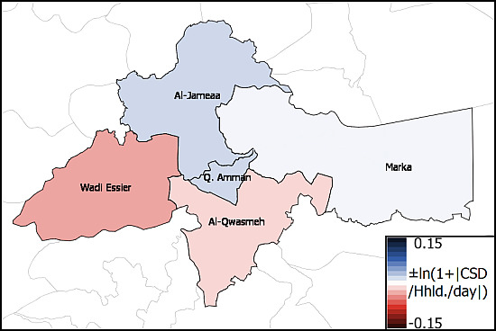
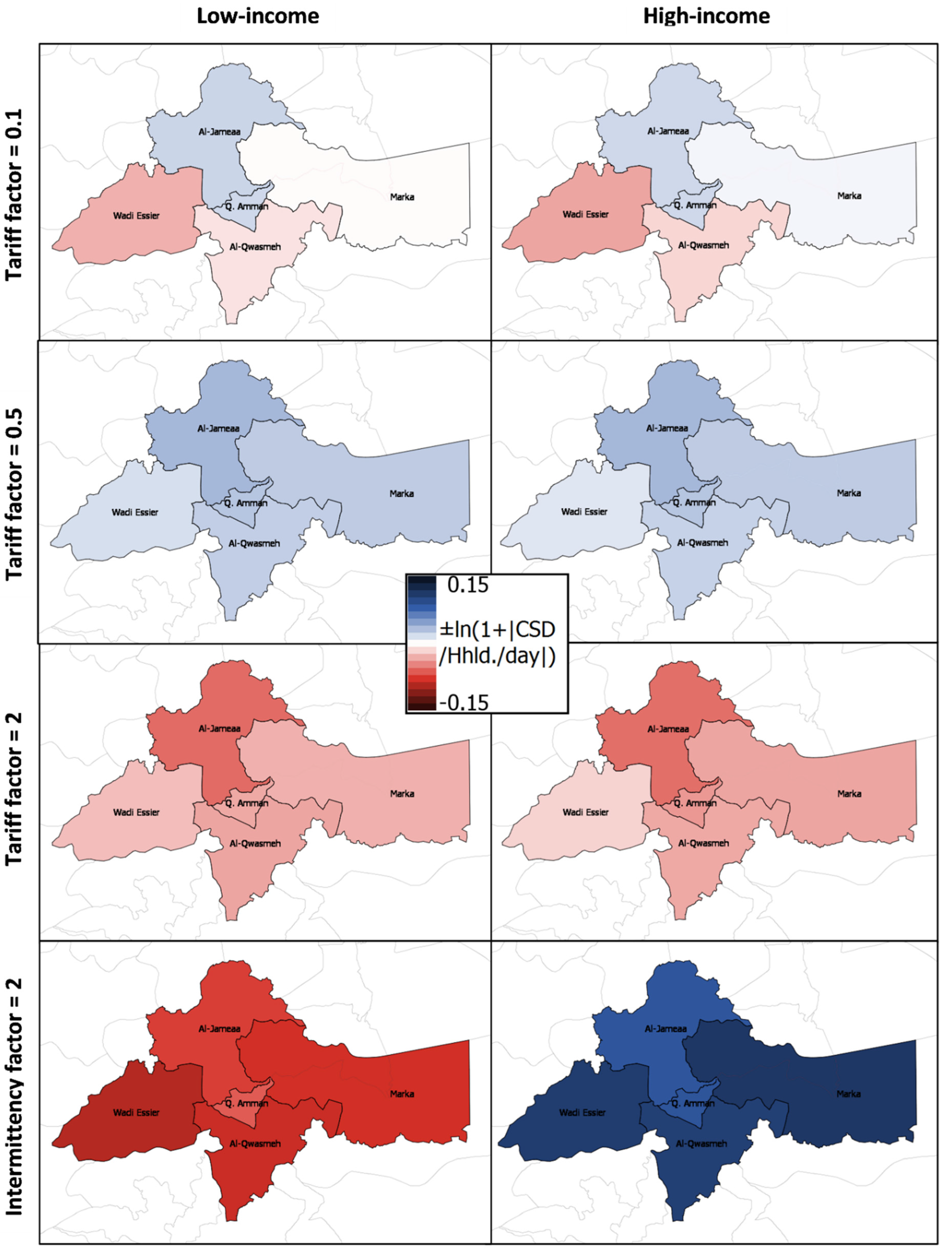
Figure 5. GIS maps showing average consumer surplus deviations from the baseline value due to changes in the piped water tariff and intermittency factors for households in different districts and income groups. Blue = gain; red = loss; darker colors indicate higher deviations from the baseline values, measured on a log-scale.

Figure 5. GIS maps showing average consumer surplus deviations from the baseline value due to changes in the piped water tariff and intermittency factors for households in different districts and income groups. Blue = gain; red = loss; darker colors indicate higher deviations from the baseline values, measured on a log-scale.

Increasing supply intermittency (Scenario 7) also creates winners and losers, though not differentiated by district, but by income class. The effects of this scenario are almost a zero-sum game and hardly as small as they seem. While the total consumer surplus difference is −2292 JD per day, high-income households gain a total of 18,905.556 JD per day and low-income households lose 21,197.531 JD per day. The reason is again the fact mentioned in Section 6.1: that most low-income households start to reach their storage constraint, switching to tanker water and thus freeing up piped water for the high-income households. Interestingly, reducing intermittency by half has no effect. The explanation for this is that, in this case as well as in the baseline, no storage constraints are met. This means that all households are able to store enough water to satisfy their demands throughout the supply breaks.

Finally, decreasing the overall availability in the piped water system (Scenario 8) naturally leads to a uniform consumer surplus loss across all agents. The decreased availability of relatively cheap piped water decreases the overall water consumption quantity and increases expenditure. This result, however, does not allow us to draw conclusions with regard to the overall welfare effect of decreasing the total water supply quantity. Since the model does not include the cost of supplying water, its implications are limited to the distribution of benefits from water consumption.

7. Discussion

The simulation results highlight the importance of a spatially and socially disaggregated perspective on the consumer surplus effects of demand-side policies and related supply-side scenarios. The first notable result is the significant size of the upper-bound estimate for the tanker water quantity throughout the different scenarios. This indicates that the tanker market is in fact very relevant in balancing the shortcomings of the piped water system.

This balancing role of tanker water is also confirmed by the substantial impact of the tanker price on consumer surplus. Despite the fact that the piped water tariff has a higher political relevance, the tanker price actually has the larger effect on consumer surplus since it is the marginal good for most households in the scenarios tested. This implies that any regulation affecting tanker water supply, be it changing the bulk water price at licensed wells or even just a stronger enforcement of rules against the illegal provision of tanker water, can potentially cause significant adverse consumer surplus impacts. This finding indicates a conflict with the objective of reducing illegal water abstractions in the interest of sustainability. A resolution of this conflict might be found in well-targeted approaches, avoiding excessive burdens on specifically vulnerable groups in society. Our analyses indicate that the strongest impact of changes in the tanker water supply conditions is found among households in parts of the city facing very high intermittency, such as the districts Qasabet Amman and Wadi Essier, whereas the income group plays a smaller role. It is, however, likely that socio-economic factors not included in the model might lead to an increased vulnerability of low-income households. Policy decisions affecting tanker water supply could benefit from considering these geographical and social vulnerabilities based on disaggregated impact analyses.

Another relevant finding in this regard is that, in the current situation, the quantity of tanker water consumed actually decreases with increases in the piped water tariff. Tariff increases lead to a more equal distribution of piped water and thereby take pressure of the households most reliant on tanker water. This finding indicates that tariff increases might actually benefit freshwater sustainability in two ways: firstly, by making households internalize some of the full costs of piped water provision and, secondly, by reducing their demand for partially unregulated tanker water. An important implication is that tariff increases can effectively be used to reduce the overall quantity of freshwater used, even when the piped water tariff is below the level where it can influence the rationed piped water consumption directly. From a purely environmental perspective, tariff increases should therefore always be worthwhile. With regards to the social impacts, however, Scenario 4 showed that a seemingly straight-forward tariff reduction can create winners and losers among districts, even when only households’ consumer surplus is considered. Under different circumstances, such a heterogeneous distribution of effects could also occur with a tariff increase. While adequate water pricing can improve the long-term sustainability and welfare contribution of the water sector, these efficiency effects are not immediately visible. In contrast, the unequal distribution of the costs imposed by demand-side measures across society is much more tangible, potentially creating problems of equity and political feasibility. This indicates that a disaggregated perspective could be beneficial for demand-side policies as well. It could help to identify measures that mitigate excessive burdens that might arise during a transition phase to more sustainable consumption patterns. These measures could range from the standard economic recommendation of targeted lump-sum transfers to more complex measures, such as a restructuring of the tariff scheme, which could distribute the projected burdens more equitably.

In all scenarios analyzed, the total piped water availability constrained the water use of some agents. In contrast, the storage constraint was not binding for any households in the baseline scenario. This result is, however, consistent with theoretical expectations. Since small storages are relatively inexpensive, households facing a binding storage constraint would likely have already expanded their capacity. A different situation arises in the intermittency scenario. Here, low-income households’ current storage does not provide sufficient flexibility to avoid negative impacts from the changed circumstances. This effect is so strong that, under a constant total water quantity, high-income households in all districts benefit substantially from the additional water that low-income households are not able to store. Given time, most low-income households would likely adapt their capacity to the situation of heightened intermittency. The implication is, however, that a sudden increase in intermittency could lead to a transition phase in which low-income households are severely affected. If the increased intermittency is foreseeable, it might be possible to mitigate this effect by means of targeted efforts, such as ensuring acceptable supply to the most vulnerable households or supporting them in extending their storage capacities in time.

8. Conclusions

The analyses above have shown that the demand-side policies necessary for sustainable water use in Jordan can have very diverse effects on different districts and socio-economic groups. In our case study of the Greater Amman Municipality, this was a direct result of including complex aspects of the water supply system, such as intermittency, in-house storage, and additional water from private tanker operators, and thus accounting for the heterogeneity among households in the city. Thereby, the particular vulnerabilities of two districts in Amman to policies affecting tanker water supply could be identified, and some unexpected results were encountered, including the fact that seemingly unambiguous policies can create spatial and socio-economic patterns of winners and losers. The model has also shown a promising approach to estimating water quantities sold on the informal water tanker market in Amman and other places featuring a similar water supply situation. Further investigations into the cost structure of water tanker operators could improve these results. Both strands of investigation, estimating tanker water quantities and simulating disaggregated policy effects across consumer groups will be further pursued in the context of the Jordan Water Project.

References and Notes

1. Rosenberg, D.E.; Talozi, S.; Lund, J.R. Intermittent water supplies: Challenges and opportunities for residential water users in Jordan. Water Int. 2008, 33, 488–504. [Google Scholar] [CrossRef]
2. The term “non-observed” has been introduced by an OECD handbook on the topic to more precisely define parts of the economy also referred to as: “hidden economy, shadow economy, parallel economy, subterranean economy, informal economy, cash economy, black market”, etc. See: Organization for Economic Co-operation and Development (OECD). Measuring the Non-Observed Economy; OECD: Paris, France, 2002; Available online: http://www.oecd.org/std/na/1963116.pdf (accessed on 25 May 2015).
3. Abu Amra, B.; Al-A’raj, A.; Al Atti, N.; Dersieh, T.; Hanieh, R.; Hendi, S.; Homoud, F.; Hussein, Y.; Jaloukh, R.; Rayyan, N. Amman Water Supply Planning Report, Volume 3, Appendices G & H; Report prepared by CDM for the United States Agency for International Development (USAID), the Ministry of Water and Irrigation (MWI), and the Water Authority of Jordan (WAJ); USAID: Amman, Jordan, 2011. [Google Scholar]
4. Jordan Water Project. Available online: https://pangea.stanford.edu/researchgroups/jordan/ (accessed on 25 May 2015).
5. Ministry of Water and Irrigation (MWI). Water for Life—Jordan’s Water Strategy 2008–2022; MWI: Amman, Jordan, 2009.
6. United Nations Development Programme (UNDP). Human Development Report 2006: Beyond Scarcity—Power, Poverty and the Global Water Crisis; Palgrave Macmillan: New York, NY, USA, 2006. [Google Scholar]
7. Kubursi, A.; Grover, V.; Darwish, A.R.; Deutsch, E. Water Scarcity in Jordan: Economic Instruments, Issues and Options; The Economic Research Forum (ERF) Working Paper 599; ERF: Cairo, Egypt, 2011. [Google Scholar]
8. Ministry of Planning and International Cooperation and United Nations (MPIC and UN). Needs Assessment Review of the Impact of the Syrian Crisis on Jordan; Host Community Support Platform (HCSP) Report. HCSP: Amman, Jordan, 2013. Available online: http://www.hcspjordan.org/s/Needs-Assessment-Review_Jordan.pdf (accessed on 25 May 2015).
9. Bonn, T. On the political sideline? The institutional isolation of donor organizations in Jordanian hydropolitics. Water Policy 2013, 15, 728–737. [Google Scholar] [CrossRef]
10. Humpal, D.; El-Naser, H.; Irani, K.; Sitton, J.; Renshaw, K.; Gleitsmann, B. Review of Water Policies in Jordan and Recommendations for Strategic Priorities: Final report; United States Agency for International Development (USAID): Washington, DC, USA, 2012.
11. French Development Agency (FDA/AFD). Jordan Water Demand Management Study; Report prepared for the Ministry of Water and Irrigation of Jordan (MWI). FDA/AFD: Paris, France, 2011. Available online: http://cmimarseille.org/cmiarchive/_src/EW2_wk1/EW2_wk1_JordanFinalReport.pdf (accessed on 25 May 2015).
12. Yorke, V. Politics Matter: Jordan’s Path to Water Security Lies through Political Reforms and Regional Cooperation; Swiss National Centre of Competence in Research (NCCR) Working Paper No. 2013/19; NCCR: Bern, Switzerland, 2013. [Google Scholar]
13. Al-Kharabsheh, A.; Ta’any, R. Challenges of Water Demand Management in Jordan. Water Int. 2005, 30, 210–219. [Google Scholar] [CrossRef]
14. Salman, A.; Al-Karablieh, E.K.; Haddadin, M.A. Limits of pricing policy in curtailing household water consumption under scarcity conditions. Water Policy 2008, 10, 295–304. [Google Scholar] [CrossRef]
15. Tabieh, M.; Salman, A.; Al-Karablieh, E.; Al-Qudah, H.; Al-Khatib, H. The Residential Water Demand Function in Amman-Zarka Basin in Jordan. Wulfenia J. 2012, 19, 324–333. [Google Scholar]
16. Coulibaly, L.; Jakus, P.M.; Keith, J.E. Modeling water demand when households have multiple sources of water. Water Resour. Res. 2014, 50, 6002–6014. [Google Scholar] [CrossRef]
17. Kariuki, M.; Schwartz, J. Small-Scale Private Service Providers of Water Supply and Electricity: A Review of Incidence, Structure, Pricing and Operating Characteristics; World Bank Policy Research Working Paper 3727; World Bank: Washington, DC, USA, 2005. [Google Scholar]
18. Opryszko, M.C.; Huang, H.; Soderlund, K.; Schwab, K.J. Data gaps in evidence-based research on small water enterprises in developing countries. J. Water Health 2009, 7, 609–622. [Google Scholar] [CrossRef] [PubMed]
19. Rosenberg, D.E.; Tarawneh, T.; Abdel-Khaleq, R.; Lund, J.R. Modeling integrated water user decisions in intermittent supply systems. Water Resour. Res. 2007, 43. [Google Scholar] [CrossRef]
20. Srinivasan, V.; Gorelick, S.M.; Goulder, L. Sustainable urban water supply in south India: Desalination, efficiency improvement, or rainwater harvesting? Water Resour. Res. 2010, 46. [Google Scholar] [CrossRef]
21. Srinivasan, V.; Gorelick, S.M.; Goulder, L. Factors determining informal tanker water markets in Chennai, India. Water Int. 2010, 35, 254–269. [Google Scholar] [CrossRef]
22. Page, S.E. Agent-based models. In The New Palgrave Dictionary of Economics, 2nd ed.; Durlauf, S.N., Blume, L.E., Eds.; Palgrave Macmillan: London, UK, 2008; Available online: http://www.dictionaryofeconomics.com/article?id=pde2008_A000218 (accessed on 25 May 2015).
23. Epstein, J.M. Generative Social Science: Studies in Agent-Based Computational Modeling; Princeton University Press: Princeton, NJ, USA, 2006; pp. 4–46. [Google Scholar]
24. Department of Statistics (DOS). Jordan Statistical Yearbook 2013; Issue No. 64; DOS: Amman, Jordan, 2013. Available online: http://www.dos.gov.jo/ (accessed on 25 May 2015).
25. Ministry of Water and Irrigation and Ministry of Planning and International Cooperation (MWI and MPIC). Quantification of the Impact of Syrian Refugees on the Water Sector in Jordan. In Proceedings of the High Level Conference on Jordan’s Water Crisis, Amman, Jordan, 2 December 2013; MWI: Amman, Jordan, 2013. [Google Scholar]
26. Potter, R.B.; Darmame, K.; Barham, N.; Nortcliff, S. “Ever-growing Amman”, Jordan: Urban expansion, social polarisation and contemporary urban planning issues. Habitat Int. 2009, 33, 81–92. [Google Scholar] [CrossRef]
27. Potter, R.B.; Darmame, K.; Nortcliff, S. Issues of water supply and contemporary urban society: the case of Greater Amman, Jordan. Philos. Trans. R. Soc. A Math. Phys. Eng. Sci. 2010, 368, 5299–5313. [Google Scholar] [CrossRef] [PubMed]
28. Potter, R.B.; Darmame, K. Contemporary social variations in household water use, management strategies and awareness under conditions of “water stress”: The case of Greater Amman, Jordan. Habitat Int. 2010, 34, 115–124. [Google Scholar] [CrossRef]
29. Gerlach, E.; Franceys, R. Regulating water services for the poor: The case of Amman. Geoforum 2009, 40, 431–441. [Google Scholar] [CrossRef]
30. Water Authority of Jordan (WAJ). Water and Wastewater Tariff for Quarterly Bills for Governorates which are Managed by Companies 2012; WAJ: Amman, Jordan, 2012. Available online: http://www.waj.gov.jo/ (accessed on 25 May 2015).
31. Theodory, G. Willingness and Ability of Residential and Non-Residential Subscribers in Greater Amman to Pay More for Water: A Study Conducted for the Water Authority of Jordan; Prepared for the United States Agency for International Development (USAID); Development Alternatives, Inc. (DAI): Amman, Jordan, 2000; p. 237. Available online: http://pdf.usaid.gov/pdf_docs/pnacq616.pdf (accessed on 25 May 2015).
32. Wildmann, T. Water Market System in Balqa, Zarqa,& Informal Settlements of Amman & the Jordan Valley—Jordan; Oxfam: Oxford, UK, 2013. [Google Scholar]
33. Department of Statistics (DOS). Table 3.12: Average Annual Current Income of Household Member by Source, Governorate and Urban/Rural (in JD). In Household Expenditure & Income Survey 2010; DOS: Amman, Jordan, 2010. Available online: http://www.dos.gov.jo/ (accessed on 25 May 2015). [Google Scholar]
34. Department of Statistics (DOS). Table 4.2: Distribution of Jordanian Population Living in Jordan Aged 5-29 Years Who Enrolled in Educational Institutions by Grade, Educational Stage, Sex and Governorates. In Population and Housing Census 2004; DOS: Amman, Jordan, 2004. Available online: http://www.dos.gov.jo/ (accessed on 25 May 2015). [Google Scholar]
35. Al-Najjar, F.O.; Al-Karablieh, E.K.; Salman, A. Residential Water Demand Elasticity in Greater Amman Area. Jordan J. Agric. Sci. 2011, 7, 93–103. [Google Scholar]
36. Miyahuna. Customer Demand Profile; Miyahuna: Amman, Jordan, 2008. [Google Scholar]
37. GIMP Home Page. Available online: http://www.gimp.org/ (accessed on 25 May 2015).
38. Potter, R.B.; Darmame, K. Contemporary social variations in household water use, management strategies and awareness under conditions of “water stress”: The case of Greater Amman, Jordan. Habitat Int. 2010, 34, 115–124, (118). [Google Scholar] [CrossRef]
39. Taylor, L.D. The Demand for Electricity: A Survey. Bell J. Econ. 1975, 6, 74–110. [Google Scholar] [CrossRef]
40. Nordin, J.A. A proposed modification of Taylor’s demand analysis: Comment. Bell J. Econ. 1976, 7, 719–721. [Google Scholar] [CrossRef]
41. Billings, R.B.; Agthe, D.E. Price elasticities for water: A case of increasing block rates. Land Econ. 1980, 56, 73–84. [Google Scholar] [CrossRef]
42. Wilensky, U. NetLogo; Center for Connected Learning and Computer-Based Modeling. Northwestern University: Evanston, IL, USA, 1999. Available online: http://ccl.northwestern.edu/netlogo/ (accessed on 25 May 2015).
43. Mulligan, M.; Wainwright, J. Modelling and Model Building. In Environmental Modelling: Finding Simplicity in Complexity; Wainwright, J., Mulligan, M., Eds.; John Wiley and Sons: Chichester, UK, 2004; pp. 7–74. [Google Scholar]