Extraction and Preference Ordering of Multireservoir Water Supply Rules in Dry Years

Abstract

This paper presents a new methodology of combined use of the nondominated sorting genetic algorithm II (NSGA-II) and the approach of successive elimination of alternatives based on order and degree of efficiency (SEABODE) in identifying the most preferred multireservoir water supply rules in dry years. First, the suggested operation rules consists of a two-point type time-varying hedging policy for a single reservoir and a simple proportional allocation policy of common water demand between two parallel reservoirs. Then, the NSGA-II is employed to derive enough noninferior operation rules (design alternatives) in terms of two conflicting objectives (1) minimizing the total deficit ratio (TDR) of all demands of the entire system in operation horizon, and (2) minimizing the maximum deficit ratio (MDR) of water supply in a single period. Next, the SEABODE, a multicriteria decision making (MCDM) procedure, is applied to further eliminate alternatives based on the concept of efficiency of order k with degree p. In SEABODE, the reservoir performance indices and water shortage indices are selected as evaluation criteria for preference ordering among the design alternatives obtained by NSGA-II. The proposed methodology was tested on a regional water supply system with three reservoirs located in the Jialing River, China, where the results demonstrate its applicability and merits.

1. Introduction

At present, China is facing a serious situation with increasing frequency of water shortage caused by high population growth and limited water resources. The problem gets even worse in dry years and has become a major bottleneck inhibiting sustainable economic and social developments. As is known to all, reservoirs play a significant role in regulating the fluctuant surface runoff to stably supply water for human needs. Actually, the design and optimization of reservoir water supply operation rules can yield the greatest benefit and least loss under drought conditions.

In previous studies, several types of water supply operation rules for guiding reservoir releases to meet planned demands have been suggested, such as the standard operating policy (SOP) [1,2], the linear decision rule (LDR) [3], the parametric rule [4], and diverse forms of hedging policy [5,6,7,8]. Among the operation rules mentioned above, the hedging policy can avoid one potential catastrophic deficit of large magnitude that may occur in future by allowing a sequence of smaller deficits in current periods [9] and has been widely applied for managing single reservoir water supply operations during drought periods [5,8,9,10,11,12]. However, multireservoir systems with water supply tasks often have complex structures of more than one reservoir in series or parallel topologies and numerous parameter variables. The design of multireservoir operation rules is a challenging work. In this study, a kind of multireservoir water supply rules integrating the hedging policy and a proportional allocation policy of downstream common water demand between two parallel reservoirs is designed for management of a multireservoir water supply system.

Additionally, it is necessary to consider different objectives simultaneously in reservoir operation models; it is noteworthy that multiobjective evolutionary algorithms (MOEAs) especially the NSGA-II algorithm, have shown excellent performance in extracting the optimal reservoir operation rules [11,13]. However, former researchers focused most of their attentions on the reservoir optimal operations [14,15] or techniques for obtaining the noninferior set that contains numbers of various multireservoir operation rules [11,13,16,17,18]. Few works on further preference ordering to reduce the scope of choices for decision makers were carried out. Therefore, the main purpose of this paper is to propose a new framework that tries solving such problems. The proposed framework includes two parts: (1) a multireservoir optimization model employing the NSGA-II for deriving a set of noninferior design alternatives of operation rules; and (2) a preference ordering procedure based on Pareto domination theories and evaluation criteria to further eliminate alternatives and determine the most preferred alternatives. Two categories of evaluation criteria are introduced: the reservoir performance indices and the shortage indices of water supply.

The remainder of this paper is organized as follows. Firstly, the problem of operation rules optimization of a multireservoir water supply system is formulated in Section 2.1. The NSGA-II algorithm and its implementation to solve the problem are also specified in this section. Secondly, the SEABODE approach is illustrated in details in Section 2.2. Thirdly, Section 2.3 shows the clear framework of the proposed methodology. Thereafter, Section 3 and Section 4 demonstrate the application study and result analysis. Finally, the paper concludes with Section 5.

2. Methodology

2.1. Optimization of Multireservoir Water Supply System

2.1.1. Hedging Policy for Single Reservoir Operations

Hedging policies are primarily designed for reservoirs to rationally allocate the limited water resources in drought conditions. By water rationing in filling or emptying or both phases of the reservoir water supply operation, the hedging policy can smooth fluctuations in water deficits and avoid unacceptable single period shortages of high percentage that may occur in future. The three most common forms of hedging policy are: (1) continuous hedging, where the slope of the hedging portion can vary continuously [7]; (2) zone-based hedging, where hedging values are a series of discrete proportions of target demands for different zones of water availability [9]; and (3) two-point type hedging, where a linear hedging policy (slope < 1) connects a first point somewhere up from the origin on the shortage portion of the SOP rule to a second point occurring on the target release line [6,19]. However, whatever the form of hedging rules, the following two critical questions must to be answered: (1) when to hedge? and (2) how much to hedge? A two-point type hedging policy, developed by Srinivasan and Philipose [6], which is characterized by three constant parameters (fixed values for the whole year), namely, starting water availability (SWA, above which the release is to be hedged), ending water availability (EWA, at which hedging is stopped) and hedging factor (HF, degree of hedging), gives an ideal answer to the two questions. 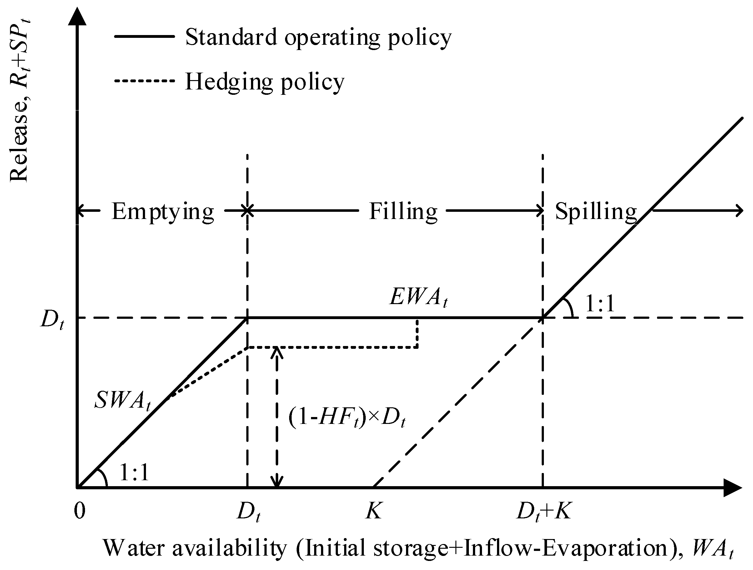In this section, an extended version of the two-point type hedging policy that considers the temporal variation (i.e., parameters SWA, EWA, and HF are varying with time) is employed as the operation rules for guiding releases of a single reservoir, as illustrated in Figure 1.

Figure 1. Two-point type time-varying hedging policy for a single period.

Figure 1. Two-point type time-varying hedging policy for a single period.

For a reservoir with water supply purpose, the water availability in period t is defined as

$$W{A}_t=S_t+Q_t-E_t$$

(1)

where $W{A}_t$ = water availability in period $t$; $S_t$ = active storage in reservoir at the beginning of period $t$, which is constrained between empty and the reservoir active capacity $K$, i.e., $0\le S_t\le K$; $Q_t$ = predicted inflow to reservoir in period $t$; and $E_t$ = water loss volume in period $t$ due to evaporation and seepage. As is shown in Figure 1, the reservoir release volume in each time period $t$ is determined according to what phase $W{A}_t$ is in and the three time-varying parameters ($SW{A}_t$, $EW{A}_t$, $H{F}_t$). The mathematical expressions of the employed hedging rules for a single reservoir are as follows.

For $W{A}_t<D_t$, i.e., in the emptying phase

$$\begin{array}{c}\begin{array}{cc}{R}_t=W{A}_t,S{P}_t=0,& \text{if} W{A}_t<SW{A}_t,\end{array}\\ \begin{array}{cc}{R}_t=SW{A}_t+\left[\left(1-H{F}_t\right)D_t-SW{A}_t\right]\frac{W{A}_t-SW{A}_t}{D_t-SW{A}_t},S{P}_t=0,& \text{otherwise}.\end{array}\end{array}$$

(2)

For $D_t\le W{A}_t\le D_t+K$, i.e., in the filling phase

$$\begin{array}{c}\begin{array}{cc}{R}_t=\left(1-H{F}_t\right)\times D_t,S{P}_t=0,& \text{if} D_t\le W{A}_t\le EW{A}_t,\end{array}\\ \begin{array}{cc}{R}_t=D_t,S{P}_t=0,& \text{otherwise}.\end{array}\end{array}$$

(3)

For $W{A}_t>D_t+K$, i.e., in the spilling phase

$$R_t=D_t,S{P}_t=W{A}_t-R_t-K$$

(4)

where $D_t$ = planned or target water demand in period $t$; $R_t$ = reservoir water supply volume in period $t$, $0\le R_t\le D_t$; $S{P}_t$ = reservoir spill flow (unused release) in period $t$; $SW{A}_t$ = starting water availability at period $t$, $0\le SW{A}_t\le D_t$; $EW{A}_t$ = ending water availability at period $t$, $D_t\le EW{A}_t\le D_t+K$; and $H{F}_t$ = hedging factor, i.e., the reduction percentage, $0\le H{F}_t\le 1$, 0 denoting a null hedging (no rationing) and 1 denoting a full hedging (no release).

The storage at the end of period $t$ is computed using the continuity equation:

$$S_{t+1}=S_t+Q_t-E_t-R_t-S{P}_t$$

(5)

in which $S_{t+1}=K$, if $S_{t+1}>K$. Other basic constraints that should be considered in the optimization model are: mass balance equation for each reservoir, reservoir minimum storage constraint, and the minimum reservoir release for downstream ecological requirements.

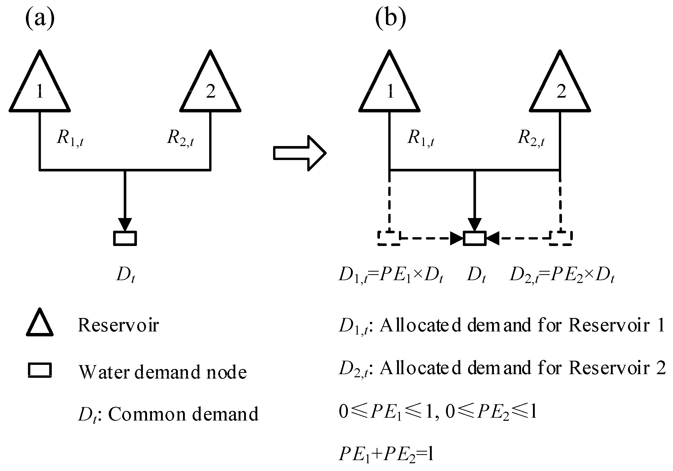
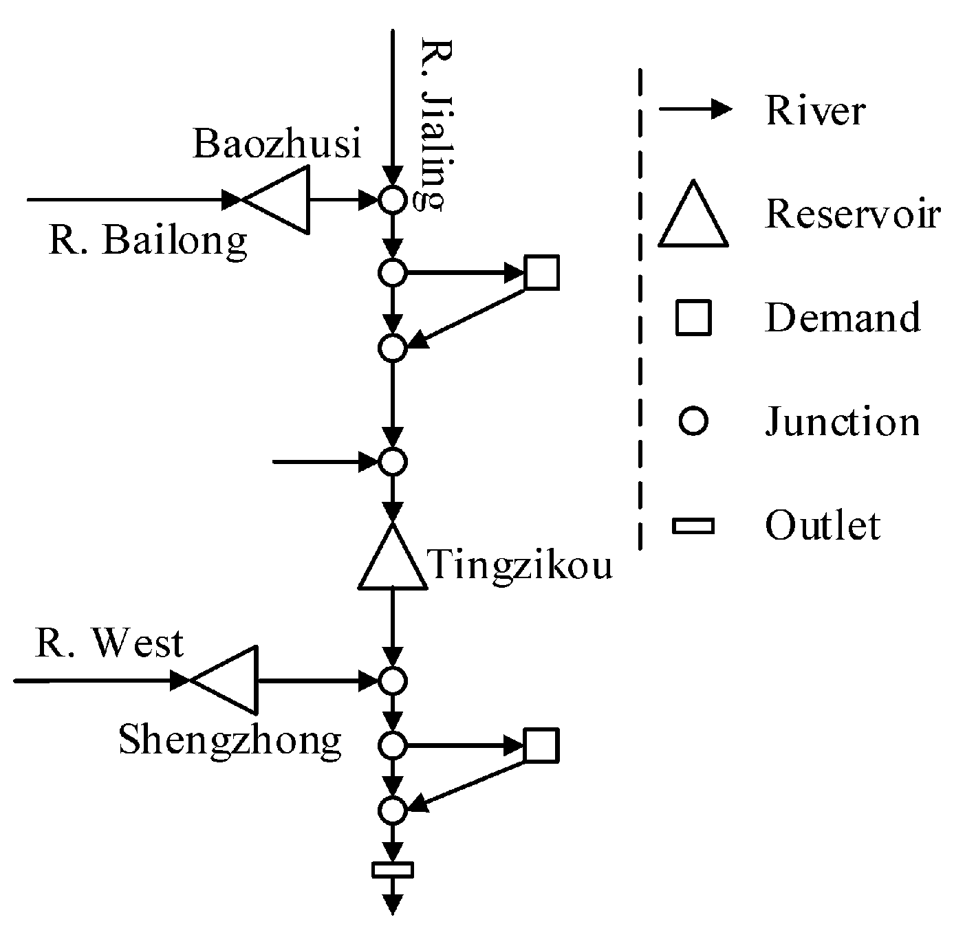
2.1.2. Allocation Policy of Common Water Demand between Parallel Reservoirs

Hedging policy can normally guide the operation of a single reservoir only when the target delivery is specified beforehand. However, for a complex multireservoir water supply system, there are always some reservoirs in parallel topology and they jointly provide downstream common water demand, which means the total amount of water supply to downstream is the summation of releases from all parallel reservoirs. It is difficult to implement hedging policy in this special configuration because the task assignment of common water demand between parallel reservoirs is inconstant and uncertain. Therefore, a proportional allocation policy is put forward to deal with this issue, shown in Figure 2. Figure 2a is the simplest two-reservoir in parallel connection; where R_1,t and R_2,t are releases from Reservoirs 1 and 2, respectively. Assume that the percentage of target demand allocated for each reservoir are PE₁ and PE₂, which are determined according to the reservoir storage capacities and respective inflow conditions. For example, PE₁ = 0.4 and PE₂ = 0.6. Then the water supply target for Reservoir 1 is D_1,t = PE₁ × D_t and D_2,t = PE₂ × D_t for Reservoir 2 shown as Figure 2b. For a parallel configuration with more than two reservoirs, the allocation policy of D_t is also in proportion.

Figure 2. (a) The parallel two-reservoir system; (b) allocation policy of common water demand.

Figure 2. (a) The parallel two-reservoir system; (b) allocation policy of common water demand.

2.1.3. Objective Functions

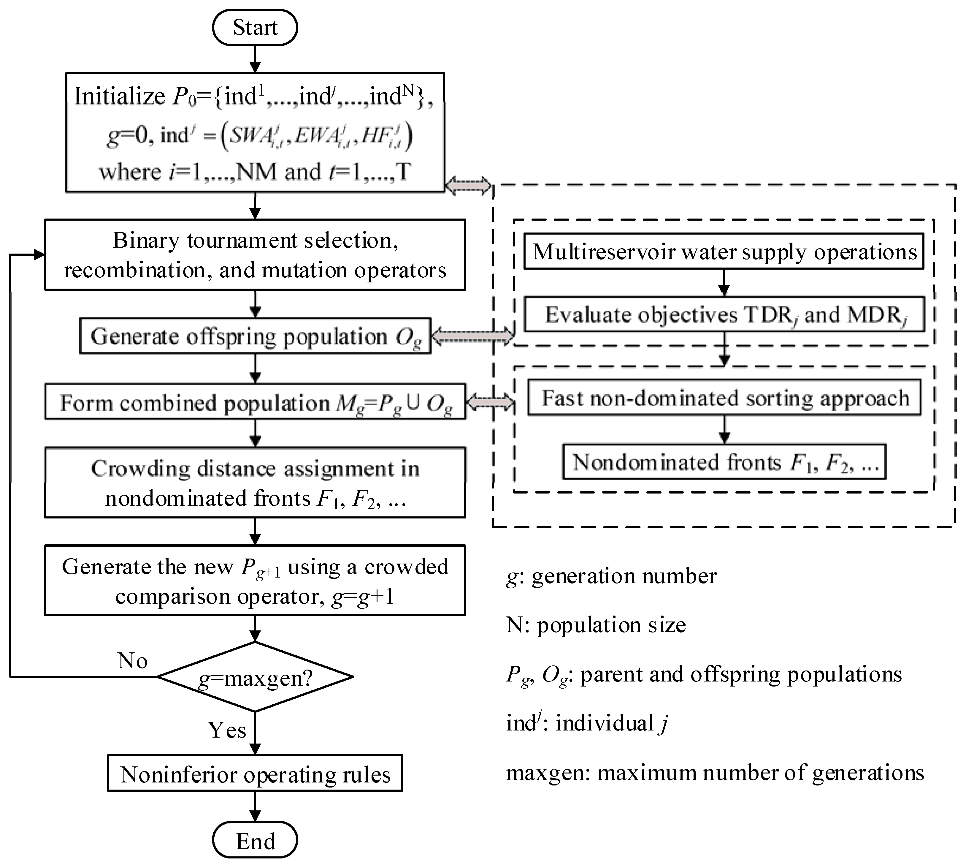
Suppose a system with NM water supply reservoirs and i denote the reservoir index, i = 1, 2, ..., NM. The allocation policy helps determine the allocated demand task D_i,t for each parallel reservoir i by the coefficient PE_i and planned common water demand. Then reservoirs could operate in order according to their respective time-varying hedging rules, represented by a parameter vector (SWA_i,t, EWA_i,t, HF_i,t). So, in optimization of a multireservoir water supply system, our purpose is to find the optimal hedging policy that makes the system perform best. Two objective functions are concerned: (1) minimizing the total deficit ratio (TDR) of all demands of the entire system in operation horizon and (2) minimizing the maximum deficit ratio (MDR) of water supply in a single period.

A deficit occurs when the reservoir releases for water supply is insufficient. The total deficit ratio of the system is defined as the ratio of total water supply deficits to the total projected demands over the operation horizon, which is expressed as

$$\text{TDR}=\frac{{\displaystyle \sum _{t=1}^{\mathrm{T}}{\displaystyle \sum _{i=1}^{\text{NM}}\left(D_{i,t}-R_{i,t}\right)}}}{{\displaystyle \sum _{t=1}^{\mathrm{T}}{\displaystyle \sum _{i=1}^{\text{NM}}{D}_{i,t}}}}\times 100\%$$

(6)

where T is the length of operation periods.

To guard against unacceptable deficits of large magnitude, minimizing single-period deficit is also important during droughts.

$$\text{MDR}=\underset{\forall i,t}{\text{Max}}\left\{\frac{D_{i,t}-R_{i,t}}{D_{i,t}}\times 100\%\right\}$$

(7)

Actually, objectives TDR and MDR are conflicting: reservoir release for water demand at each time period should be as full as possible to minimize MDR, but no hedging would induce frequent deficit events and sacrifice long-term water supply reliability, which may increase TDR; conversely, satisfying the TDR would enlarge the MDR [11,18].

2.1.4. Solution Technique to Extract Design Alternatives

The NSGA-II, developed by Deb et al. [20], is one of the most efficient and steady population-based MOEAs and has been widely reported by various investigators in solving water resource systems-related problems. Some recent applications are: parameter calibration of hydrologic models [21,22], optimal design and management of flood control on watershed scale [23,24], reservoir systems optimization [14,25,26,27], and extraction of optimal operation policies [13]. 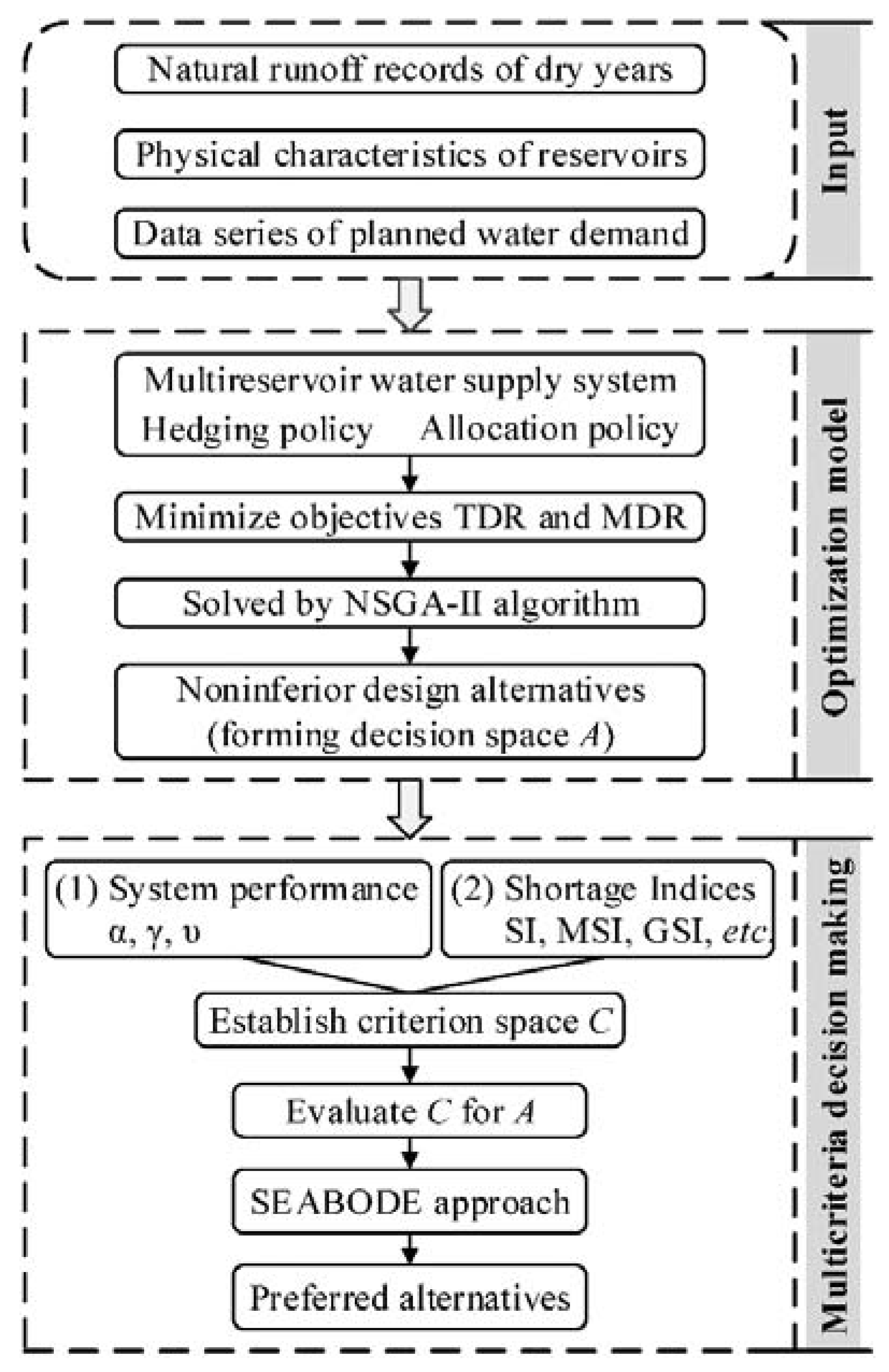Figure 3 shows the flowchart of applying the NSGA-II to derive a noninferior set of operation rules for a multireservoir water supply system. The main steps are summarized as follows:

Step 1: Create initial parent population $P_0$ of size $\mathrm{N}$ and set the generation number $g=0$; the $j\text{th}$ individual ${\text{ind}}^j$ represents a scheme of hedging policy, i.e., variables $SW{A}_{i,t}^j$, $EW{A}_{i,t}^j$, $H{F}_{i,t}^j$ with $t=1,\mathrm{...},\mathrm{T}$ and $i=1,\mathrm{...},\text{NM}$.

Step 2: For different ${\text{ind}}^j$ in $P_0$, implement the water supply operations of reservoirs one by one, then calculate objectives ${\text{TDR}}_j$ and ${\text{MDR}}_j$.

Step 3: Sort $P_0$ based on non-domination and assign a rank to each individual equal to its non-domination level (1 is the best level, 2 is the next-best level, and so on).

Step 4: Generate an offspring population $O_g$ of size $\mathrm{N}$ using binary tournament selection, crossover, and mutation operators.

Step 5: Evaluate offspring population $O_g$; the same as step 2.

Step 6: Combine the parent and offspring population to form a mating pool $M_g$ of size $2\mathrm{N}$, $M_g=P_g\cup O_g$.

Step 7: Sort $M_g$ by the fast non-dominated sorting algorithm to identify all non-dominated fronts $F_1$,$F_2$,…

Step 8: Estimate the crowding distance of each individual in different non-dominated fronts (crowding-distance-assignment).

Step 9: Perform the crowded comparison operator on $M_g$ to generate a new parent population, $P_{g+1}$.

Step 10: Set $g=g+1$, and go to Step 4. Repeat steps 4–9 until the stopping criterion is satisfied ($g=\max \text{gen}$).

Figure 3. Flowchart to optimize a multireservoir water supply system using the NSGA-II.

Figure 3. Flowchart to optimize a multireservoir water supply system using the NSGA-II.

2.2. Preference Ordering according to Quantitative Criteria

Now a set (the decision space) that includes N noninferior design alternatives of operation rules in terms of objectives TDR and MDR will be presented to decision makers. However, the size is too large to choose. Further eliminating some alternatives and setting up a preference ordering among the remainder are necessary. In general, none of these alternatives can be pronounced better than others in the absence of more information. Therefore, it is practicable to consider several relevant quantitative criteria so as to evaluate and rank them.

2.2.1. Evaluation Criteria

Two types of quantitative evaluation criteria are used for assessing different design alternatives: reservoir performance indices mainly contain reliability α, resiliency γ, and vulnerability υ [7]; shortage indices of water supply such as shortage index (SI) or modified SI (MSI) [28], deficit percent day index (DPD), and generalized shortage index (GSI) [29].

Reservoir Performance Indices

Reliability α describes how likely a system is to fail; resilience γ indicates how quickly it recovers from failure; and vulnerability υ measures how severe the consequences of failure may be. They are defined as Equations (8)–(10).

$$\mathsf{\alpha }=1-\frac{\underset{t=1}{\overset{\text{TN}}{\Pi }}\left(D_t>R_t\right)}{\text{TN}}$$

(8)

$$\mathsf{\gamma }=\frac{\underset{t=1}{\overset{\text{TN}-1}{\Pi }}\left(D_{t+1}\le R_{t+1}|D_t>R_t\right)}{\underset{t=1}{\overset{\text{TN}}{\Pi }}\left(D_t>R_t\right)}$$

(9)

$$\mathsf{\upsilon }=\underset{t=1}{\overset{\text{TN}}{\text{max}}}\left(\frac{D_t-R_t}{D_t}|D_t>R_t\right)$$

(10)

where TN = length of periods in counting; $\underset{t=1}{\overset{\text{TN}}{\Pi }}\left(D_t>R_t\right)$ = count of periods in which target demands are not fully satisfied; $\underset{t=1}{\overset{\text{TN}-1}{\Pi }}\left(D_{t+1}\le R_{t+1}|D_t>R_t\right)$ = count of events that reservoir success to supply target demand after a failure state; and $\underset{t=1}{\overset{\text{TN}}{\text{max}}}\left(\frac{D_t-R_t}{D_t}|D_t>R_t\right)$ = maximum relative deficit in the failure periods.

Shortage Indices

The shortage index (SI), introduced by the U.S. Army Corps of Engineers to indicate the degree of water shortage [30], and the modified shortage index (MSI) are defined in Equations (11) and (12), respectively.

$$\text{SI}=\frac{100}{\mathrm{Y}}{\displaystyle \sum {\left(\frac{\text{Annual} \text{water} \text{deficit}}{\text{Planned} \text{annual} \text{demand}}\right)}^2}$$

(11)

$$\text{MSI}=\frac{100}{\mathrm{T}}{\displaystyle \sum _{t=1}^{\mathrm{T}}{\left(\frac{{\text{TS}}_t}{{\text{TD}}_t}\right)}^2}$$

(12)

where Y = the number of sample years; ∑ = the summation of the indicated values for all deficit periods; TS_t = shortage in period t; TD_t = demand in period t; and T = number of periods.

The deficit duration is the total time of a continuous drought event; the deficit intensity is the average of deficit in the event. They are also vital to water resources planning. The deficit percent day index (DPD) includes these two characteristics:

$$\text{DPD}={\displaystyle \sum \left[\text{Daily} \text{deficit} \text{rate}(\%)\times \text{Number} \text{of} \text{days} \text{in} \mathrm{a} \text{continuous} \text{deficit}\right]}$$

(13)

where ∑ represents the summation of the indicated values for all deficit events in the period under consideration. The generalized shortage index (GSI) not only incorporates all essential aspects of SI and DPD, but also emphasizes the consequential socioeconomic impacts of water supply. It can be expressed as follows:

$$\text{GSI}=\frac{100}{\mathrm{Y}}{\displaystyle \sum _{i=1}^{\mathrm{Y}}{\left(\frac{{\text{DPDa}}_i}{100\times {\text{DY}}_i}\right)}^{\mathsf{\beta }}}$$

(14)

where Y = number of sample years; β = coefficient, usually taken as 2; DY_i = number of days in the ith year (365 or 366); and DPDa_i = sum of all DPDs in the ith year.

2.2.2. The SEABODE Approach

There are a number of approaches to evaluate different design alternatives according to multiple criteria, and they can be classified into two categories: aggregation approaches and Pareto domination approaches. The former is to form a “scalarization” form of multiple evaluation criteria and rank the alternatives based on this specific scalar, such as the conversion tools of weighted sum [31], distance function [32], and utility function [33]. However, the results may be highly sensitive to the scalarization method we used and there is no well-defined means of picking the right scalarization. Besides, due to some subjective factors of decision makers, the aggregation approach cannot always guarantee that all final choices are strictly reasonable. However, in contrast, a Pareto domination approach, called successive elimination of alternatives based on order and degree of efficiency (SEABODE), does not need to specify weigh coefficients to any evaluation criterion and can overcome the drawbacks of aggregation approaches [34]. The SEABODE is based on two theorems: efficiency of order k and efficiency of order k with degree p. For a feasible set of a large number of design alternatives, the SEABODE to select the preferred alternatives involves two steps: (1) find all alternatives belonging to the same lowest order of efficiency, recorded as k_min; (2) among the result set, only retain the alternatives that are efficient of order (k_min − 1) with highest degree p_max. Definitions of the two domination theorems used in the SEABODE approach are given as follows.

Efficiency of Order k

An alternative is defined as being efficient of order k or k-Pareto-optimal, if it is not dominated by any other alternatives for all the possible k-dimensional subspace of the original m-dimensional criterion space C (1 ≤ k ≤ m).

Efficiency of Order k with Degree p

Assume that there are a number of (k + 1)-Pareto-optimal alternatives, but none of them is k-Pareto-optimal. An alternative is defined as efficiency of order k with degree p if it is not dominated by any other alternatives for the exact p k-dimensional subspaces of C and is denoted as [k, p]-Pareto-optimal.

2.2.3. Numerical Illustration

Table 1 shows a set of 10 design alternatives (a1–a10) in a three-dimensional criterion space C = (c1–c3) as a numerical illustration, where c1–c3 are minimized. It can be clearly seen from Table 1 that all 10 design alternatives are 3-Pareto-optimal because no one can fully dominate the others. For example, the values of criteria c1 and c2 for a2 are both larger than those of a1, but the value of criterion c3 of a2 is lower than that of a1, which indicates that neither a1 or a2 dominates the other totally. Figure 4 plotted the alternatives from Table 1 in two-dimensional criterion subspace for the possible combinations of any two of the three criteria in C. In Figure 4, alternatives surrounded by circles are Pareto-optimal in their respective two-dimensional criterion subspace. As can be seen from Figure 4a, a1, a3, and a7 are on the Pareto front of criteria c1 versus c2; criteria c1 versus c3 in Figure 4b has four 2-Pareto-optimal alternatives (a7–a10); c3 versus c2 in Figure 4c has six 2-Pareto-optimal alternatives (a1, a2, a5–a8). Through the analysis, k_min = 3, p_max = 3, a7 is the most preferred choice.

Table 1. Numerical values of all three criteria for each alternative.

Alternatives	Criteria (m = 3)			3-Pareto-Optimal	[k, p]-Pareto-Optimal
	c1	c2	c3		[2,1]	[2,2]	[2,3]
a1	6.33	2.45	51.31	√	√	√
a2	13.91	3.68	36.54	√	√
a3	4.12	6.01	58.15	√	√
a4	8.62	7.57	46.22	√
a5	12.35	9.74	32.13	√	√
a6	10.11	11.96	23.15	√	√
a7	1.05	15.51	15.20	√	√	√	√ (preferred)
a8	5.71	26.53	5.22	√	√	√
a9	2.43	31.26	13.84	√	√
a10	3.57	43.22	9.01	√	√

Table 1. Numerical values of all three criteria for each alternative.

Alternatives	Criteria (m = 3)			3-Pareto-Optimal	[k, p]-Pareto-Optimal
	c1	c2	c3		[2,1]	[2,2]	[2,3]
a1	6.33	2.45	51.31	√	√	√
a2	13.91	3.68	36.54	√	√
a3	4.12	6.01	58.15	√	√
a4	8.62	7.57	46.22	√
a5	12.35	9.74	32.13	√	√
a6	10.11	11.96	23.15	√	√
a7	1.05	15.51	15.20	√	√	√	√ (preferred)
a8	5.71	26.53	5.22	√	√	√
a9	2.43	31.26	13.84	√	√
a10	3.57	43.22	9.01	√	√

Figure 4. Two-dimensional Pareto plots of the three criteria: (a) c1 versus c2; (b) c1 versus c3; (c) c3 versus c2.

Figure 4. Two-dimensional Pareto plots of the three criteria: (a) c1 versus c2; (b) c1 versus c3; (c) c3 versus c2.

2.3. Framework of the Proposed Methodology in Application

As shown in Figure 5, application of the proposed methodology to determine the optimal operation rules for a multireservoir water supply system in dry years is manipulated according to the following three steps: (1) an input module (a process of data preparation); (2) an optimization model using the NSGA-II algorithm to derive a number of noninferior hedging policies in terms of objectives TDR and MDR, which forms the decision space A; (3) a MCDM procedure to further select the most preferred alternatives according to criterion space C and the SEABODE approach.

Figure 5. Framework to select preferred operation rules in application.

Figure 5. Framework to select preferred operation rules in application.

3. Case Study

3.1. System Description

Jialing River is a major tributary of the Yangtze River in China. A regional water supply system with three reservoirs (Baozhusi, Tingzikou, and Shengzhong) located in the upper and middle reaches of the Jialing River is employed as a case study. Figure 6 is the layout of the investigated system. As shown in Figure 6, Tingzikou is a leading water conservancy project in the mainstream of the Jialing River; Baozhusi and Shengzhong are two smaller reservoirs in tributaries, Bailong River and West River, respectively. Some critical parameters of the three reservoirs are listed in Table 2. The flood season is concentrated from June to August.

Figure 6. Sketch map of the investigated system.

Figure 6. Sketch map of the investigated system.

Table 2. Reservoir characteristic parameters.

Reservoir	Active Storage Capacity K (102 Million m3)		PE (Predefined)
	Normal Season (September–May)	Flood Season (June–August)
Baozhusi	13.40	10.58	-
Tingzikou	17.32	4.72	0.7
Shengzhong	6.72	6.72	0.3

Table 2. Reservoir characteristic parameters.

Reservoir	Active Storage Capacity K (102 Million m3)		PE (Predefined)
	Normal Season (September–May)	Flood Season (June–August)
Baozhusi	13.40	10.58	-
Tingzikou	17.32	4.72	0.7
Shengzhong	6.72	6.72	0.3

3.2. Dry Years and Water Demand Data

The Changjiang Institute of Survey, Planning, Design and Research provided all input data including runoff records of typical years and water demand target data [35]. As inflows to reservoirs, monthly runoff series for 50 years (from 1959 to 2008) were collected and are sufficient to characterize the varying hydrological regime of the Jialing River.

The division of water years was based on the specific guaranteed rate (GR) of annual runoff series at a watershed mainstream control station. Specifically, the water years were divided into exceptionally wet years (GR < 12.5%), slightly wet years (12.5% ≤ GR < 37.5%), normal years (37.5% ≤ GR ≤ 62.5%), slightly dry years (62.5% < GR ≤ 87.5%), and exceptionally dry years (GR > 87.5%) [36]. Figure 7 shows the annual natural runoff series in ascending rank. The first 20 dry years (five exceptionally dry years and 15 slightly dry years) were selected for demonstration, resulting in Y = 20 hydrological scenarios of different degrees of drought, or 240 operation periods in total for the optimization model (T = 240). Since the 20 dry years are not continuous, the optimization model needs to be run for each (dry) year separately (12 months) in calculations. The water demand series in different months of one dry year are predicted data for future planning horizon (level year of 2020). The reservoir evaporation losses are roughly equal to the average reservoir water-spread areas multiplying the evaporation rate in one period. The seepage loss is neglected. Table 3 shows the average inflows of the demonstration dry years and the target demands data in 2020 level for each reservoir.

Figure 7. Annual runoff series in ascending rank (1959–2008).

Figure 7. Annual runoff series in ascending rank (1959–2008).

Table 3. Average natural inflows of the demonstration dry years (Y = 20) and corresponding target demands in 2020 level year (m³/s).

	Reservoir	Months
		January	February	March	April	May	June	July	August	September	October	November	December
Average Inflows	Baozhusi	202.3	180.3	185.8	289.7	472.8	532.7	754.9	684.6	681.6	512.4	318.6	222.9
	Shengzhong	106.1	92.5	101.3	184.7	301.2	345.3	502.7	537.8	508.7	350.1	200.1	132.2
	Tingzikou	257.7	197.1	230.3	415.9	670.6	686.1	1691.3	1266.4	1342.9	653.0	467.8	317.5
Demands (2020)	Baozhusi	39.5	51.2	48.4	52.9	54.9	67.6	54.2	49.7	33.9	39.6	41.0	39.8
	Shengzhong	106.4	111.3	114.4	98.3	291.9	237.7	179.1	169.1	78.6	72.4	86.1	127.0
	Tingzikou	159.6	167.0	171.6	147.4	437.9	356.5	268.7	253.6	117.9	108.6	129.1	190.5

Table 3. Average natural inflows of the demonstration dry years (Y = 20) and corresponding target demands in 2020 level year (m³/s).

	Reservoir	Months
		January	February	March	April	May	June	July	August	September	October	November	December
Average Inflows	Baozhusi	202.3	180.3	185.8	289.7	472.8	532.7	754.9	684.6	681.6	512.4	318.6	222.9
	Shengzhong	106.1	92.5	101.3	184.7	301.2	345.3	502.7	537.8	508.7	350.1	200.1	132.2
	Tingzikou	257.7	197.1	230.3	415.9	670.6	686.1	1691.3	1266.4	1342.9	653.0	467.8	317.5
Demands (2020)	Baozhusi	39.5	51.2	48.4	52.9	54.9	67.6	54.2	49.7	33.9	39.6	41.0	39.8
	Shengzhong	106.4	111.3	114.4	98.3	291.9	237.7	179.1	169.1	78.6	72.4	86.1	127.0
	Tingzikou	159.6	167.0	171.6	147.4	437.9	356.5	268.7	253.6	117.9	108.6	129.1	190.5

3.3. Parameter Settings and Search Ranges of Decision Variables

In this study, parameters of the NSGA-II algorithm used to search various noninferior design alternatives are set to: population size N = 100, maximum number of generations maxgen = 1000, crossover probability p_c = 0.9, mutation probability p_m = 1/108, crossover and mutation distribution indexes η_c = 20 and η_m = 20 [20,22,23]. Moreover, a genetic algorithm (GA) with real-coded pattern and elite strategy is applied to find the extreme optimal MDR and TDR separately. The parameter setting for GA is: population size = 200, maximum number of iterations = 1000, crossover and mutation probabilities p_c = 0.9, p_m = 0.05 [11], elites to be reserved are the top 5% of individuals in each generation.

It is not realistic to adopt a large value of HF that exceeds the allowable degree of damage to the water supply. To avoid such an unreasonable result in practical applications, the search ranges of decision variables SWA, EWA, and HF are reset to [0.1D, 0.9D], [1.1D, D + K], and [0.1, 0.3], respectively [6]. In the optimization model, the time step is one month. For a single reservoir, the number of variables of monthly varying hedging rules is 36. The total number of decision variables in the optimization model equals to 108 (NM = 3).

4. Results and Discussion

Usually, for evolutionary algorithms in engineering applications, multiple trials are needed depending on two aspects: (1) the randomness and initialization, which may largely influence the performance of evolutionary algorithms; and (2) the complexity of the optimization problem. However, for the case study in this paper, optimization results (noninferior solutions) obtained by the NSGA-II between multiple trials are similar and have no obvious difference. This may be due to the model structure (only including three reservoirs and 108 decision variables) and the input data used in calculations. Furthermore, the aim of the case study is to illustrate the application process and feasibility of the proposed methodology. So, in this section, we only choose and analyze a relatively superior trial among many tries.

4.1. Decision Space Obtained by the Optimization Model

The Pareto front or the decision space A, derived by the NSGA-II algorithm, contains 100 feasible design alternatives (a1, ..., a100) that are well-distributed in the area from 8.38% to 10.00% for TDR, and from 34.59% to 63.50% for MDR, as shown in Figure 8a. The extreme values of TDR and MDR obtained by optimizations of single-objective GA are 8.30% and 34.41%, respectively, and Figure 8b gives corresponding convergence trajectories.

Figure 8. (a) The decision space A derived by NSGA-II; (b) results of single-objective optimizations obtained by GA.

Figure 8. (a) The decision space A derived by NSGA-II; (b) results of single-objective optimizations obtained by GA.

4.2. Preferred Alternatives Determined by the SEABODE

A point to note is that even after eliminating all inferior alternatives and preserving the Pareto optimal ones in terms of objectives MDR and TDR by using the NSGA-II algorithm, the decision maker is still left with a sizeable number of options to choose from (alternatives a1, ..., a100). To further pick out the preferred alternatives, the three performance indices (reliability α, resilience γ, and vulnerability υ) and the generalized shortage index (GSI) are selected and constitute a four-dimensional criterion space C for evaluating each alternative. For each reservoir in the system, variation ranges for the four criteria by statistical results from the 100 alternatives in decision space A are listed in Table 4. It can be seen from Table 4 that: (1) all values of the four selected criteria for Baozhusi are constant among all the 100 alternatives, implying no preferences exist between different alternatives for Baozhusi; (2) variation ranges of the four criteria for Shengzhong and Tingzikou fluctuate obviously, largely affected by different alternatives. Therefore, we chose Shengzhong and Tingzikou as the analysis objects to apply the SEABODE approach and determine the preferred alternative for each reservoir.

Table 4. Statistics of the specified evaluation criteria for each reservoir in decision space A.

Reservoir		Four-Dimensional Criterion Space C
		1-α	2-γ	3-υ	4-GSI
Baozhusi	Range	= 1	= 1	= 0	= 0
	Std.	–	–	–	–
Shengzhong	Range	[0.658, 0.825]	[0.297, 0.637]	[0.345, 0.520]	[0.203, 0.541]
	Std.	0.054	0.079	0.061	0.112
Tingzikou	Range	[0.592, 0.842]	[0.342, 0.665]	[0.346, 0.635]	[0.434, 1.487]
	Std.	0.092	0.097	0.089	0.336

Table 4. Statistics of the specified evaluation criteria for each reservoir in decision space A.

Reservoir		Four-Dimensional Criterion Space C
		1-α	2-γ	3-υ	4-GSI
Baozhusi	Range	= 1	= 1	= 0	= 0
	Std.	–	–	–	–
Shengzhong	Range	[0.658, 0.825]	[0.297, 0.637]	[0.345, 0.520]	[0.203, 0.541]
	Std.	0.054	0.079	0.061	0.112
Tingzikou	Range	[0.592, 0.842]	[0.342, 0.665]	[0.346, 0.635]	[0.434, 1.487]
	Std.	0.092	0.097	0.089	0.336

Table 5 gives the number of Pareto-optimal alternatives in the original four-dimensional criterion space and its four subspaces of any three criteria. It can be observed from Table 5 that (1) for Shengzhong, only 29 alternatives are Pareto-optimal if all four evaluation criteria are considered, i.e., 71 alternatives, about 71% of the decision space A are eliminated; (2) for Tingzikou, 31 inferior alternatives, about 31% of the decision space A are eliminated. However, one must be able to sieve through these alternatives to obtain a smaller number of representative alternatives. Table 6 shows applications of the SEABODE approach on the remainder of 4-Pareto-optimal alternatives for Shengzhong and Tingzikou. It is clearly seen in Table 6 that as the degree (p) of any order increases, the number of preferred alternative decreases or does not change. Take for example Shengzhong, where we see that the number of preferred alternatives decreases from 29 to 5 when the degree of order 3 increases from 1 to 4, while the number reduces from 5 to 1 when the degree of order 2 increases from 1 to 6. Thus the number of alternatives becomes small but the qualities are still good (they are of the highest degree and a high order of efficiency, i.e., [2,6]-Pareto-optimal alternative a86). The same analysis can be applied for Tingzikou and the finally selected preferred alternative is a54 ([2,4]-Pareto-optimal alternative).

Table 5. Number of Pareto-optimal alternatives in all possible three-dimensional subspaces of C.

Reservoir	C	Three-dimensional subspaces
	(1-2-3-4)	(1-2-3)	(1-2-4)	(1-3-4)	(2-3-4)
Shengzhong	29	15	7	28	29
Tingzikou	69	18	2	63	63

Note: 1-α, 2-γ, 3-υ, 4-GSI.

Table 5. Number of Pareto-optimal alternatives in all possible three-dimensional subspaces of C.

Reservoir	C	Three-dimensional subspaces
	(1-2-3-4)	(1-2-3)	(1-2-4)	(1-3-4)	(2-3-4)
Shengzhong	29	15	7	28	29
Tingzikou	69	18	2	63	63

Note: 1-α, 2-γ, 3-υ, 4-GSI.

Table 6. Preferred alternatives resulting from the SEABODE approach.

Reservoir	4-Pareto	[3,1]	[3,2]	[3,3]	[3,4]	[2,1]	[2,2]	[2,3]	[2,4]	[2,5]	[2,6]
Shengzhong	29	29	28	14	5	5	5	5	5	2	1
Tingzikou	69	68	60	17	0	17	15	9	1	0	0

Table 6. Preferred alternatives resulting from the SEABODE approach.

Reservoir	4-Pareto	[3,1]	[3,2]	[3,3]	[3,4]	[2,1]	[2,2]	[2,3]	[2,4]	[2,5]	[2,6]
Shengzhong	29	29	28	14	5	5	5	5	5	2	1
Tingzikou	69	68	60	17	0	17	15	9	1	0	0

Table 7 shows a comparison between the results of the finally selected preferred alternatives and the optimal results by optimizing single objective MDR or TDR. As can be expected, values of MDR and TDR of preferred alternatives a86 and a54 are generally within the range of the corresponding values of single objective optimizations. The preferred alternatives a86 and a54 are not only noninferior alternatives in terms of MDR and TDR but also the alternatives that can make Shengzhong and Tingzikou have good performance in reservoir performance indices and GSI.

Table 7. Results of the preferred alternative and single objective optimizations.

		GA-MDR	GA-TDR	NSGA-II + SEABODE
				Shengzhong (a86)	Tingzikou (a54)
Objectives	MDR (%)	34.41	68.76	56.13	60.30
	TDR (%)	19.16	8.30	8.51	8.42
Shengzhong	α	0.379	0.825	0.825	0.821
	γ	0.159	0.529	0.529	0.504
	υ	0.320	0.494	0.494	0.520
	GSI	3.371	0.200	0.204	0.204
Tingzikou	α	0.296	0.842	0.804	0.842
	γ	0.164	0.648	0.610	0.665
	υ	0.344	0.688	0.561	0.603
	GSI	4.316	0.482	0.597	0.440

Table 7. Results of the preferred alternative and single objective optimizations.

		GA-MDR	GA-TDR	NSGA-II + SEABODE
				Shengzhong (a86)	Tingzikou (a54)
Objectives	MDR (%)	34.41	68.76	56.13	60.30
	TDR (%)	19.16	8.30	8.51	8.42
Shengzhong	α	0.379	0.825	0.825	0.821
	γ	0.159	0.529	0.529	0.504
	υ	0.320	0.494	0.494	0.520
	GSI	3.371	0.200	0.204	0.204
Tingzikou	α	0.296	0.842	0.804	0.842
	γ	0.164	0.648	0.610	0.665
	υ	0.344	0.688	0.561	0.603
	GSI	4.316	0.482	0.597	0.440

4.3. Areas for Future Research

Some improved versions of NSGA, such as epsilon-NSGA-II [37] or BORG [38], have been proposed recently. Although these newly developed evolutionary algorithms were regarded as more efficient in theory and mathematical experiments, there are few case studies applying them in practical engineering, especially for BORG. Moreover, the most important innovation of this research is the novel methodology we proposed on preference ordering for the reduction of the scope of multi-reservoir operation choices. Since NSGA-II (also an improved version of NSGA) has been widely used by various investigators in solving water resource systems-related problems and is a mature technique, we employed it to derive noninferior solutions. However, trying these modified algorithms in our extensive research is a very attractive direction for us to take in the future.

Originally, when we conceived and designed the methodology, it was quite natural to consider the allocation ratio PE_i,t (i is the reservoir index of parallel reservoirs, t is the time index) as decision variables. However, we noted that the variation ranges of the decision variables SWA_i,t (0 ≤ SWA_i,t ≤ D_i,t) and EWA_i,t (D_i,t ≤ EWA_i,t ≤ D_i,t + K_i) are associated to PE_i,t because D_i,t = PE_i,t × D_t (D_t is the water demand in period t and its value is known beforehand). That way, the boundaries on SWA_i,t and EWA_i,t vary with the value of PE_i,t during iterative computations of NSGA-II; even the initial solutions are produced in different search spaces depending on the randomly generated PE_i,t. There are correlations between some decision variables, which makes the optimization problem very complicated and varying (violating the consistency requirement for optimization problems). This type of problem is seldom seen in multiobjective optimizations. For most applications of multiobjective evolutionary algorithms (MOEAs), the search spaces of decision variables are fixed. Thereupon, fixed PE_i,t values were used in our study, which were determined according to the reservoir storage capacities and average reservoir inflow conditions. We and maybe other researches are expecting to see PE_i,t as decision variables and explore new techniques to deal with constraints of this type that are dynamically changing. This is another interesting area for future research.

5. Summary and Conclusions

A few conclusions arising out of this paper are listed as follows:

• A simple multireservoir operation policy includes the hedging policy for water supply operation of a single reservoir and the proportional allocation policy of downstream common water demand between two parallel reservoirs is suggested by the authors.
• A new methodology, which aims at deriving a certain number of noninferior multireservoir water supply rules in dry years or drought conditions and making a preference ordering among the extracted alternatives according to several specified evaluation criteria, is proposed. The proposed methodology is implemented as the following two main steps (1) an optimization model of multireservoir operation using the NSGA-II algorithm to obtain a number of noninferior hedging rules in terms of objectives TDR and MDR, which forms a decision space containing enough design alternatives for decision makers to choose between; and (2) a multicriteria decision-making procedure to further eliminate the alternatives according to the SEABODE approach.
• In order to illustrate the application and effect of the proposed methodology, the three-reservoir water supply system in Jialing River is employed as a case study. Results show that we can always find the preferred alternative among a sizeable number of noninferior alternatives for each reservoir with the help of the SEABODE approach. The proposed methodology was able to sieve through the numerous noninferior alternatives and short-list a small number of preferred alternatives to present to decision makers for further consideration.

References

1. Maass, A.; Hufschmidt, M.M.; Dorfman, R.; Thomas, H.A., Jr.; Marglin, S.A.; Fair, G.M. Design of Water-Resource Systems; Harvard University Press: Cambridge, MA, USA, 1962. [Google Scholar]
2. Stedinger, J.R. The performance of LDR models for preliminary design and reservoir operation. Water Resour. Res. 1984, 20, 215–224. [Google Scholar] [CrossRef]
3. Revelle, C.; Joeres, E.; Kirby, W. The linear decision rule in reservoir management and design: 1, Development of the stochastic model. Water Resour. Res. 1969, 5, 767–777. [Google Scholar] [CrossRef]
4. Nalbantis, I.; Koutsoyiannis, D. A parametric rule for planning and management of multiple-reservoir systems. Water Resour. Res. 1997, 33, 2165–2177. [Google Scholar] [CrossRef] [Green Version]
5. Shih, J.-S.; ReVelle, C. Water-supply operations during drought: Continuous hedging rule. J. Water Resour. Plan. Manag. 1994, 120, 613–629. [Google Scholar] [CrossRef]
6. Srinivasan, K.; Philipose, M.C. Evaluation and selection of hedging policies using stochastic reservoir simulation. Water Resour. Manag. 1996, 10, 163–188. [Google Scholar] [CrossRef]
7. Hashimoto, T.; Stedinger, J.R.; Loucks, D.P. Reliability, resiliency, and vulnerability criteria for water resource system performance evaluation. Water Resour. Res. 1982, 18, 14–20. [Google Scholar] [CrossRef]
8. Neelakantan, T.R.; Pundarikanthan, N.V. Hedging rule optimisation for water supply reservoirs system. Water Resour. Manag. 1999, 13, 409–426. [Google Scholar] [CrossRef]
9. Shih, J.-S.; ReVelle, C. Water supply operations during drought: A discrete hedging rule. Eur. J. Oper. Res. 1995, 82, 163–175. [Google Scholar] [CrossRef]
10. Felfelani, F.; Movahed, A.J.; Zarghami, M. Simulating hedging rules for effective reservoir operation by using system dynamics: A case study of Dez Reservoir, Iran. Lake Reserv. Manag. 2013, 29, 126–140. [Google Scholar] [CrossRef]
11. Shiau, J.-T. Optimization of reservoir hedging rules using multiobjective genetic algorithm. J. Water Resour. Plan. Manag. 2009, 135, 355–363. [Google Scholar] [CrossRef]
12. Tu, M.; Hsu, N.; Yeh, W. Optimization of reservoir management and operation with hedging rules. J. Water Resour. Plan. Manag. 2003, 129, 86–97. [Google Scholar] [CrossRef]
13. Ahmadi, M.; Haddad, O.B.; Mariño, M.A. Extraction of flexible multi-objective real-time reservoir operation rules. Water Resour. Manag. 2014, 28, 131–147. [Google Scholar] [CrossRef]
14. Scola, L.A.; Neto, O.M.; Takahashi, R.H.C.; Cerqueira, S.A.A.G. Multi-objective optimal multiple reservoir operation. In Proceedings of the 2011 IEEE Congress on Evolutionary Computation, New Orleans, LA, USA, 5–8 June 2011; pp. 1927–1933.
15. Ngo, L.L.; Madsen, H.; Rosbjerg, D. Simulation and optimisation modelling approach for operation of the Hoa Binh reservoir, Vietnam. J. Hydrol. 2007, 336, 269–281. [Google Scholar] [CrossRef]
16. Afshar, A.; Sharifi, F.; Jalali, M.R. Non-dominated archiving multi-colony ant algorithm for multi-objective optimization: Application to multi-purpose reservoir operation. Eng. Optim. 2009, 41, 313–325. [Google Scholar] [CrossRef]
17. Afshar, M.H. Large scale reservoir operation by constrained particle swarm optimization algorithms. J. Hydro-Environ. Res. 2012, 6, 75–87. [Google Scholar] [CrossRef]
18. Guo, X.; Hu, T.; Wu, C.; Zhang, T.; Lv, Y. Multi-objective optimization of the proposed multi-reservoir operating policy using improved NSPSO. Water Resour. Manag. 2013, 27, 2137–2153. [Google Scholar] [CrossRef]
19. Bayazit, M.; Ünal, N.E. Effects of hedging on reservoir performance. Water Resour. Res. 1990, 26, 713–719. [Google Scholar] [CrossRef]
20. Deb, K.; Pratap, A.; Agarwal, S.; Meyarivan, T. A fast and elitist multiobjective genetic algorithm: NSGA-II. IEEE Trans. Evol. Comput. 2002, 6, 182–197. [Google Scholar] [CrossRef]
21. Khu, S.T.; Madsen, H. Multiobjective calibration with Pareto preference ordering: An application to rainfall-runoff model calibration. Water Resour. Res. 2005, 41. [Google Scholar] [CrossRef]
22. Bekele, E.G.; Nicklow, J.W. Multi-objective automatic calibration of SWAT using NSGA-II. J. Hydrol. 2007, 341, 165–176. [Google Scholar] [CrossRef]
23. Yazdi, J.; Salehi Neyshabouri, S.A.A. Optimal design of flood-control multi-reservoir system on a watershed scale. Nat. Hazards 2012, 63, 629–646. [Google Scholar] [CrossRef]
24. Yazdi, J.; Salehi-Neyshabouri, S.A.A. A simulation-based optimization model for flood management on a watershed scale. Water Resour. Manag. 2012, 26, 4569–4586. [Google Scholar] [CrossRef]
25. Hosseini, P.; Chen, D.; Leon, A.S. Optimizing short-term operation of a multireservoir system during transition of objectives and constraints. In Proceedings of the World Environmental and Water Resources Congress 2014, Portland, OR, USA, 1–5 June 2014; pp. 1093–1105.
26. Suen, J.-P.; Eheart, J.W. Reservoir management to balance ecosystem and human needs: Incorporating the paradigm of the ecological flow regime. Water Resour. Res. 2006, 42. [Google Scholar] [CrossRef]
27. Yin, X.A.; Yang, Z.F. Development of a coupled reservoir operation and water diversion model: Balancing human and environmental flow requirements. Ecol. Model. 2011, 222, 224–231. [Google Scholar] [CrossRef]
28. Hsu, N.-S.; Cheng, K.-W. Network flow optimization model for basin-scale water supply planning. J. Water Resour. Plan. Manag. 2002, 128, 102–112. [Google Scholar] [CrossRef]
29. Hsu, S.-K. Shortage indices for water-resources planning in Taiwan. J. Water Resour. Plan. Manag. 1995, 121, 119–131. [Google Scholar] [CrossRef]
30. Hydrologic Engineering Center. Reservoir Yield. In Hydrologic Engineering Methods for Water Resources Development; U.S. Army Corps of Engineers: Davis, CA, USA, 1975; Volume 8. [Google Scholar]
31. Madsen, H. Parameter estimation in distributed hydrological catchment modelling using automatic calibration with multiple objectives. Adv. Water Resour. 2003, 26, 205–216. [Google Scholar] [CrossRef]
32. Liong, S.; Khu, S.; Chan, W. Derivation of Pareto front with genetic algorithm and neural network. J. Hydrol. Eng. 2001, 6, 52–61. [Google Scholar] [CrossRef]
33. Krzysztofowicz, R.; Duckstein, L. Preference criterion for flood control under uncertainty. Water Resour. Res. 1979, 15, 513–520. [Google Scholar] [CrossRef]
34. Das, I. A preference ordering among various pareto optimal alternatives. Struct. Optim. 1999, 18, 30–35. [Google Scholar] [CrossRef]
35. Changjiang Institute of Survey, Planning, Design and Research. Report of Water Resources Assessment for the Planning of Jialing River Basin; Changjiang Water Resources Commission of the Ministry of Water Resources: Wuhan, China, 2013. [Google Scholar]
36. Ji, X.; Wang, J.; Xiong, M.; Chen, J. Hydrological Analysis, Calculation and Water Resources Assessment; China Water & Power Press: Beijing, China, 2008. [Google Scholar]
37. Tang, Y.; Reed, P.; Wagener, T. How effective and efficient are multiobjective evolutionary algorithms at hydrologic model calibration? Hydrol. Earth Syst. Sci. 2006, 10, 289–307. [Google Scholar] [CrossRef]
38. Hadka, D.; Reed, P. Borg: An auto-adaptive many-objective evolutionary computing framework. Evol. Comput. 2012, 21, 231–259. [Google Scholar] [CrossRef] [PubMed]