Assessing Variation in Water Balance Components in Mountainous Inland River Basin Experiencing Climate Change

Abstract

Quantification of the changes of water balance components is significant for water resource assessment and management. This paper employed the Soil and Water Assessment Tool (SWAT) model to estimate the water balance in a mountainous watershed in northwest China at different spatial scales over the past half century. The results showed that both Nash-Sutcliffe efficiency (NSE) and determination coefficient (R²) were over 0.90 for the calibration and validation periods. The water balance components presented rising trends at the watershed scale, and the total runoff increased by 30.5% during 1964 to 2013 period. Rising surface runoff and rising groundwater flow contributed 42.7% and 57.3% of the total rising runoff, respectively. The runoff coefficient was sensitive to increasing precipitation and was not significant to the increase of temperature. The alpine meadow was the main landscape which occupied 51.1% of the watershed and contributed 55.5% of the total runoff. Grass land, forest land, bare land, and glacier covered 14.2%, 18.8%, 15.4%, and 0.5% of the watershed and contributed 8.5%, 16.9%, 15.9%, and 3.2% of the total runoff, respectively. The elevation zone from 3500 to 4500 m occupied 66.5% of the watershed area, and contributed the majority of the total runoff (70.7%). The runoff coefficients in the elevation zone from 1637 to 2800 m, 2800 to 3500 m, 3500 to 4000 m, 4000 to 4500 m, and 4500 to 5062 m were 0.20, 0.27, 0.32, 0.43, and 0.78, respectively, which tend to be larger along with the elevation increase. The quantities and change trends of the water balance components at the watershed scale were calculated by the results of the sub-watersheds. Furthermore, we characterized the spatial distribution of quantities and changes in trends of water balance components at the sub-watershed scale analysis. This study provides some references for water resource management and planning in inland river basins.

1. Introduction

Water resources are affected by the alteration of a number of water balance components which have different responses to climate change [1,2]. Effective management of water resources in cold and alpine regions requires detailed attention to be paid to the spatial distribution of the water balance components [3,4]. Water balance components include: precipitation, evapotranspiration, total runoff, surface runoff, groundwater flow and the soil water content. The quantification of the various water balance components of hydrological processes in a watershed remains a challenging topic [5,6,7,8], because several unknown components, e.g., evapotranspiration and soil water content, included in the water balance are difficult to measure [9]. However, the calculation of water balance components is significant for water resources assessment and management especially for water-scarce regions with regard to assessment of the impact of climate change. The water balance components can be realistically simulated using a continuous watershed hydrological model [10,11,12]. Meanwhile water balance models could provide an accurate estimate of runoff, relative changes in soil moisture, evapotranspiration, etc. [13,14].

In recent years, the water balance components have been estimated at different scales based on water balance models. For example, Gregory et al. [15] simulated the water balance components at the global scale; and Herrmann et al. [16] determined the spatial difference of water balance components at the regional scale. Generally, researchers mainly focused on the water balance at the basin or the watershed scale [3,17,18]. Several studies have discussed the water balance across land cover type, vegetation pattern, and ecosystem scale. For example, Jian et al. [19] quantified the changes of each water balance component for different land cover types in a small catchment. Thompson et al. [20] proposed a synthesis framework to compute the water balance from vegetation patterns and catchment scales. Knowles et al. [21] estimated the relative contributions of the two ecosystems to the water balance. These reports facilitate our current understanding of the changes of the spatial distribution of water balance components at specific scales. However, there is a major question regarding how the relationships in water balance components vary across different spatial scales in response to climate change? Thus, a multi-scale analysis focused on changes in the spatial distribution of water balance components is necessary to fully understand the interaction between the hydrological processes and environment.

The mountainous regions in inland river basins are very sensitive to climate change [22,23,24]. We choose the upper reaches of Heihe River Basin (HRB) as the study area. The HRB is the second largest inland river basin in China. There are more than 1.3 million people and 266,000 ha of irrigated agricultural land in the middle and lower reaches of the river basin depending on the runoff coming from the upper watershed, which is crucial to maintain the oasis and agricultural ecosystems in the middle and lower reaches of the river. Because of the increasing water resources and eco-environmental problems, the HRB has attracted many researchers’ attention in China. In the HRB, there are several studies simulating hydrological processes [25,26,27,28,29,30]. However, there have been few studies conducted to estimate the climate change impact on water balance components in the mountainous watershed at different spatial scales. This study aims to understand the distribution characteristics of hydrological processes using the SWAT model and to analyze the water balance components and runoff recharge behavior at different spatial scales (watershed, landscape, elevation zones, and sub-watershed) under the background of climate change in the upper reaches of HRB, which can serve as a reference for regional water resource assessment and planning in the HRB.

2. Materials and Methods

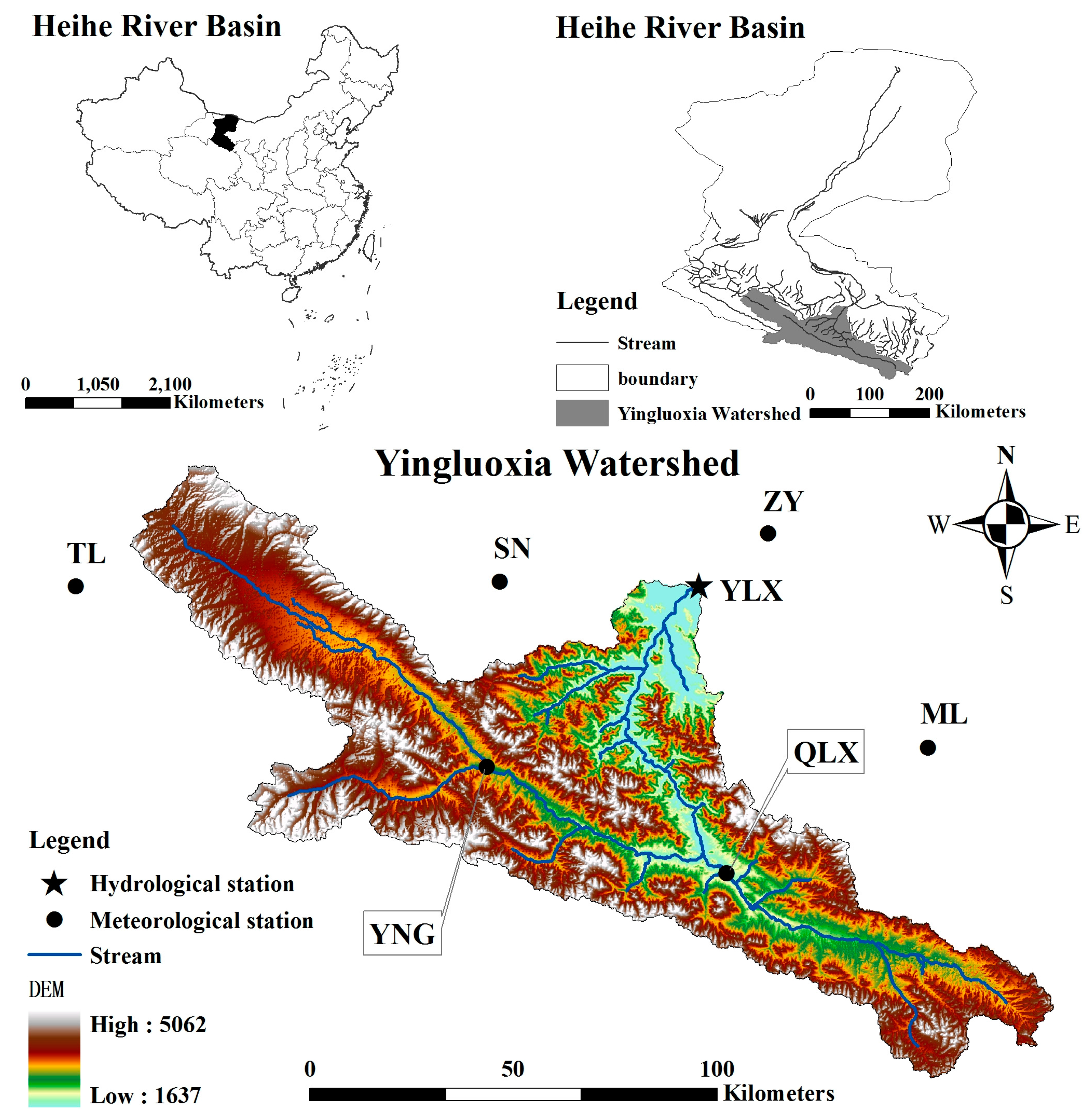
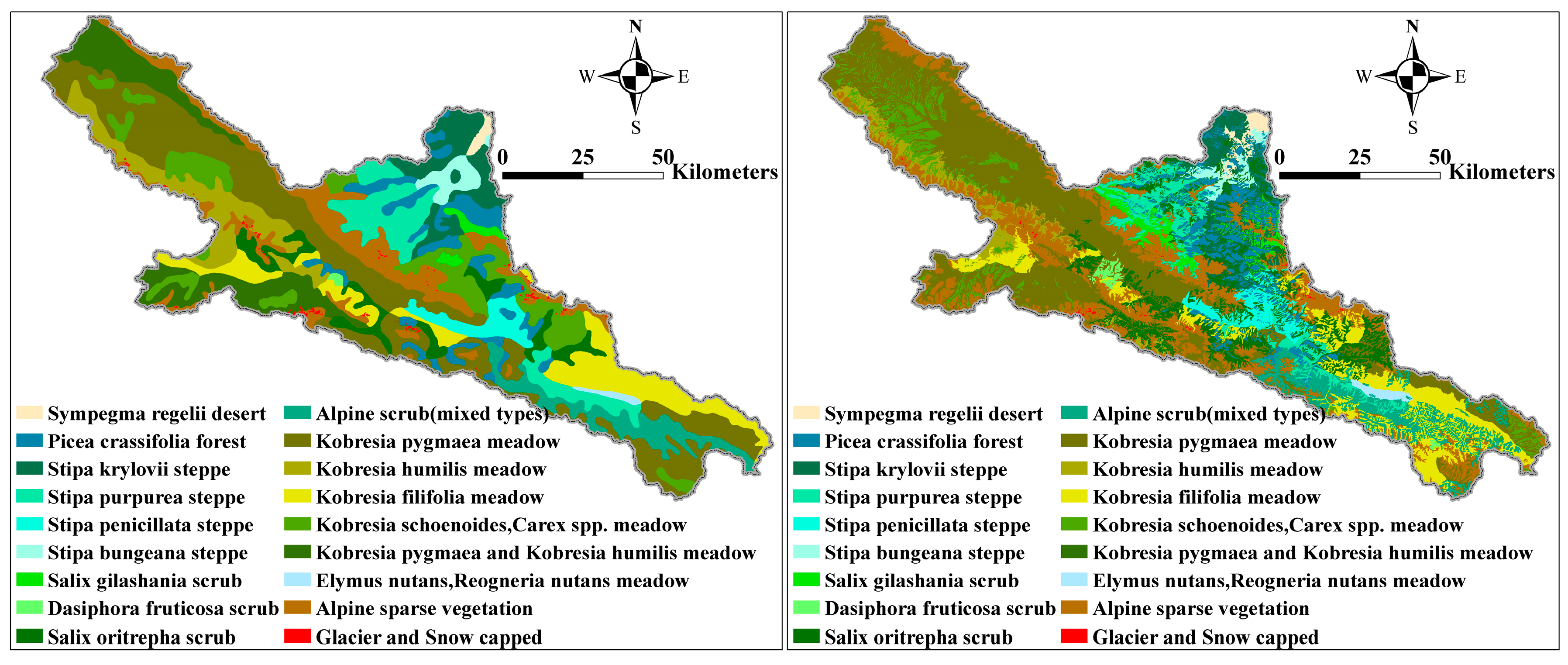
2.1. Study Area

The HRB is the second largest inland river basin in China, located in the central part of the Hexi Corridor, which used to be an important section of the ancient Silk Road. The geographical coordinates range from 98° to 101°30′ E and 38° to 42° N, which is a representative inland river basin in the semi-arid and arid regions of northwest China and covers an area of approximately 130,000 km². The Yingluoxia watershed is located at the main stream of HRB which is a mountainous watershed having an area of approximately 10,018 km², mostly comprising mountainous terrain (Figure 1). It is the main region of runoff generation in HRB. Most of the water resources in the middle oasis and lower desert ecosystem are therefore recharged by runoff from the upper reaches. The mountainous runoff of the Yingluoxia watershed is monitored by the Yingluoxia (YLX) hydrological station. The climate of the study area is warm and wet in summer and cold and dry in winter with large spatial and temporal variability. The average annual precipitation tends to increase from west to east from 200 mm to 700 mm. The precipitation mainly occurs in wet seasons usually from June to September accounting for nearly 70% of the annual precipitation, only 3.5% of the annual precipitation occurs from December to February, and less than 10% occurs from November to March. The annual air temperature of the watershed varied from −5 to 4 °C during the period from 1961 to 2013. Altitudinal landscape zones exist in the watershed, including a desert steppe zone from 1637 to 2800 m, shrubbery forest grassland zone from 2800 to 3500 m, sub-alpine shrubbery meadow zone from 3500 to 4000 m, alpine cold-and-desert meadow zone from 4000 to 4500 m, and alpine permafrost–snow–ice zone from 4500 m to 5062 m [31].

2.2. Soil and Water Assessment Tool (SWAT) Model

The SWAT model was developed by the United States Department of Agriculture. It is a semi-distributed model which is based on physical processes [32]. The model has some advantages in predicting climate change effects on water-related and hydrological processes over long periods, and it is a continuous-time, river basin scale model. The SWAT model can run with different time scales, including annual, monthly, and daily time scales [33]. In SWAT, a basin is divided into many sub-basins, which are then subdivided into many hydrologic response units (HRUs) in development that are composed of homogeneous land cover, soil type, and terrain features. The entire water balance is simulated based on each HRU, including: precipitation interception, precipitation partitioning, snowmelt water, redistribution of soil water content, evapotranspiration, lateral subsurface flow from the soil profile, and return flow from shallow aquifers.

The hydrological processes simulated by SWAT are on the basis of the following water balance equation:

$$S{W}_t=S{W}_0+{\displaystyle \sum _{i=1}^t(P_{day}-Q_s-E_a-w_{seep}-Q_g)}$$

(1)

where SW_t is the final soil water content (mm), SW₀ is the initial soil water content on day i (mm), t is the time (days), P_day is the amount of precipitation on day i (mm), Q_s is the amount of surface runoff on day i (mm), E_a is the amount of ET on day i (mm), w_seep is the amount of water entering the vadose zone from the soil profile on day i (mm), and Q_g is the amount of return flow on day i (mm).

2.3. Glacier and Snow Melt Algorithm

2.3.1. Snow Melt Algorithm

SWAT distinguishes precipitation as rain or snow by the mean daily temperature. The threshold temperature used to categorize precipitation as rain or snow is defined by the user. If the mean daily air temperature is lower than the threshold temperature, then the precipitation will be modeled as snow and the water equivalent will be added to the snow pack. If the mean daily air temperature is higher than the threshold temperature, then the precipitation will be modeled in the form of liquid rain. The snow pack will increase with additional snowfall or will decrease with snowmelt or sublimation, and the water stored in the snow pack will be reported as a snow water equivalent.

In this case study, the temperature index with elevation band approach was applied to simulate snowmelt [34,35]. The snowmelt in SWAT is calculated as a linear function of the difference between the average snow pack-maximum air temperature and the base or threshold temperature for snowmelt. The snowmelt equation on a given day is:

$$SN{O}_{mlt}=b_{mlt}\times SN{O}_{\mathrm{cov}}\times \left[\frac{T_{snow}+T_{mx}}{2}-T_{mlt,sno}\right]$$

(2)

where SNO_mlt is the amount of snowmelt (mm), b_mlt is the melt factor for the day (mm/day-°C), SNO_cov is the fraction of the HRU area covered by snow, T_snow is the snow pack temperature (°C), T_mx is the maximum air temperature (°C), and T_mlt,sno is the base temperature above which snowmelt is allowed (°C). The melt factor is allowed a seasonal variation with maximum and minimum values occurring on summer and winter solstices:

$$b_{mlt}=\frac{\left(b_{mlt6}+b_{mlt12}\right)}{2}+\frac{\left(b_{mlt6}-b_{mlt12}\right)}{2}\times \sin \left(\frac{2\pi }{365}\times \left(d_n-81\right)\right)$$

(3)

where b_mlt is the melt factor for the day (mm/day-°C), b_mlt6 is the melt factor for 21 June (mm/day-°C), b_mlt12 is the melt factor for 21 December (mm/day-°C), and d_n is the day of the year.

2.3.2. Glacier Melt Algorithm

A distributed temperature-index approach was used for glacier melt modeling. It calculates the melting of glacial ice based on a linear relationship between ablation and positive air temperature. This approach takes into account the effect of potential solar radiation, thus including the variability in topographic shading, aspect, and slope [34]. The local melt rate is calculated as:

$$M=\{\begin{array}{lll}(F_M+r_{ice}{I}_{pot})\times (T-T_{mlt,ice})& :& T>T_{mlt,ice}\\ 0& :& \mathrm{T}\le T_{mlt,ice}\end{array}$$

(4)

where F_M is the melt factor, r_ice is the ice radiation factor. I_pot denotes the potential solar direct radiation, and T is the mean daily air temperature, whereby temperature below zero indicates that no melting occurs. The potential solar direct radiation, I_pot, is a function of top-of-atmosphere solar radiation, solar geometry, topographic characteristics use, and atmospheric transmissivity:

$$I_{pot}=S{\left(\frac{d_m}{d}\right)}^2{\mathrm{\Psi }}^{\frac{P}{P_0\cos Z}}\left[\cos \mathsf{\theta }\cos Z+\sin \mathsf{\theta }\sin Z\cos \left({\mathsf{\varphi }}_{sun}-{\mathsf{\varphi }}_{slope}\right)\right]$$

(5)

where S = 1360 W·m⁻² is the solar constant, (d_m/d)² is the eccentricity correction factor of the Earth’s orbit, $\mathrm{\Psi }$ = 0.75 is the mean atmospheric clear-sky transmissivity, P is the atmospheric pressure, P₀ is the mean atmospheric pressure at sea level, Z is the zenith angle (which is approximated as a function of latitude, solar declination, and hour angle), θ is the slope angle, φ_sun is the solar azimuth angle, and φ_slope is the slope azimuth angle. Potential direct solar radiation is set to zero between sunset and sunrise and for the surface that is shaded by surrounding topography.

2.4. Data Availability

The ASTER GDEM was used as the digital elevation model (DEM) data with a 30 m resolution. The meteorological and hydrological observation data were all downloaded from the portal of Environmental and Ecological Science Data Center for West China (http://westdc.westgis.ac.cn). Two periods of vegetation map were obtained (version 1.0, 2001; version 2.0, 2014), with the vegetation types including: alpine meadow, grassland, forest land, bare land, and glacier, as shown in Figure 2. The soil map (scale 1:1,000,000) was obtained from the China Soil Scientific Database (CSSD). Related main soil properties including soil particle-size composition, soil texture, soil depth, and organic carbon content for the different layers of each soil type were obtained directly from the CSSD. Bulk density, available water capacity of the soil layer, and saturated hydraulic conductivity were calculated by a SPAW (Soil-Plant-Atmosphere-Water) model [36]. The modified logistic growth model with two parameters was used to convert the soil particle-size from international standard to the US standard [37]. The other soil properties that were difficult to be acquired were set to the default value in the SWAT soil database.

Daily weather data series: precipitation, maximum and minimum air temperature, average wind speed, relative humidity, and sunshine duration were obtained from the records of the six meteorological stations as shown in Figure 1 and

Table 1. Hydro-meteorological stations that were used in the SWAT simulation.

Station	Longitude/°	Latitude/°	Elevation/m	Period	Average Air Temperature/°C	Average Precipitation/mm
Meteorological stations
Zhangye (ZY)	E 100.38	N 38.93	1483	1961–2013	7.3	131.9
Minle (ML)	E 100.82	N 38.45	2271	1961–2013	3.4	337.1
Sunan (SN)	E 99.62	N 38.83	2312	1961–2013	3.8	250.9
Qilianxian (QLX)	E 100.25	N 38.18	2787	1961–2013	1.1	410.6
Yeniugou (YNG)	E 99.58	N 38.42	3180	1961–2013	−2.6	420.9
Tuole (TL)	E 98.42	N 38.82	3360	1961–2013	−2.5	299.9
Hydrological stations
Yingluoxia (YLX)	E 100.18	N 38.82	1637	1961–2013	-	-

. Monthly river flow data were obtained from the YLX hydrological station for the observation period from 1961 to 2013. In this study, the model was calibrated based on monthly time scale using the data from January 1961 to December 1988, and the model validated by using the data from January 1986 to December 2013 of the YLX hydrological stations. The data during January 1961 to December 1963 and January 1986 to December 1988 were set as ‘warm-up’ periods respectively for calibration and validation.

2.5. Model Setup

After preparation of forcing data, four major steps must be done to setup the model: (i) watershed discretization and sub-watershed characteristics derivation; (ii) define the HRU; (iii) run the model and analyze the parameter sensitivity; and (iv) calibrate and validate the SWAT model, including uncertainty analysis.

During the watershed delineation, we divided the YLX watershed into 43 sub-watersheds using ArcSWAT tool. The sub-watersheds water balance components were used to determine the basin-scale data in this study. In the HRU definition step, four classes of slope with large ranges 0% to 5% (7.6% of the total area), 5% to 25% (36.6% of the total area), 25% to 45% (24.5% of the total area), >45% (31.3% of the total area) were addressed because the study area is an alpine terrain with numerous rugged topographies. As a result, the whole watershed was delineated into 2650 HRUs. The entire water balance was simulated based on each HRU, and then the quantities of the water balance components were added to the outlet of the sub-watershed. The sub-watershed scale water balance components were routed to the outlet of the whole watershed (watershed scale). The third step was to run the model using the prepared weather data inputs and HRU information defined in the previous steps. The simulation was run first for the calibration period from January 1961 to December 1988. The fourth step in the modeling process was calibration and validation. The process of calibration and validation was necessary and will be detailed in the next section.

2.6. Model Calibration and Uncertainty Analysis

The Sequential Uncertainty Fitting algorithm (SUFI-2) was applied to perform the calibration and uncertainty analysis [38]. All sources of uncertainty such as the model structure, driving variables (e.g., rainfall), parameters, and measured data were included in the ranges of parameters, which were calibrated to bracket most of the measured data in 95% prediction uncertainty (95PPU). 95PPU was calculated at the 2.5% and 97.5% levels of the cumulative distribution of output variables. P-factor and R-factor were used to quantify the goodness of calibration/uncertainty performance. A P-factor is the percentage of measured data bracketed by the 95PPU band, and an R-factor is the average width of the band divided by the standard deviation of the corresponding measured variable. Theoretically, the value of the P-factor ranges between 0 and 100%, while that of R-factor ranges between 0 and infinity. A P-factor of 1 and R-factor of 0 is a simulation that exactly corresponds to the measured data.

Based on the sensitivity analysis and our previous study [26], 16 parameters were chosen, whose final fitted parameter values were shown in

Table 2. Parameters related in the calibration procedure as well as the fitted values.

Parameter 1	Description	Parameter Range	Fitted Value
r_CN2.mgt	Initial SCS runoff curve number for moisture condition II	−0.4–0.2	−0.28
v_ALPHA_BF.gw	Base flow alpha factor (days)	0.0–0.5	0.45
v_GW_DELAY.gw	Groundwater delay time (days)	90.0–180.0	174.0
v_GWQMN.gw	Threshold depth of water in the shallow aquifer required for return flow to occur (mm)	0.0–2.0	0.62
v_GW_REVAP.gw	Groundwater ‘rewap’ coefficient	0.0–0.2	0.037
v_ESCO.hru	Soil evaporation compensation factor	0.5–0.9	0.80
v_CH_N2.rte	Manning’s ‘n’ value for the main channel	0.0–0.3	0.026
v_CH_K2.rte	Effective hydraulic conductivity in main channel alluvium (mm/h)	5.0–40.0	35.0
v_ALPHA_BNK.rte	Base flow alpha factor for bank storage	0.0–1.0	0.61
r_SOL_AWC.sol	Available water capacity of the soil layer (mm H2O/mm soil)	−0.2–0.4	−0.10
r_SOL_K.sol	Saturated hydraulic conductivity (mm/h)	−0.8–0.8	−0.54
r_SOL_BD.sol	Moist bulk density (mg/m3)	−0.5–0.6	0.44
v_SFTMP.bsn	Snowfall temperature (°C)	−2.0–1.0	0.21
v_SMFMN.bsn	Melt factor on December 21 (mm H2O/°C-day)	0–10.0	3.5
v_SMFMX.bsn	Melt factor on 21 June (mm H2O/°C-day)	0–10.0	7.5
v_TLPAS.sub	Temperature lapse rate (°C/km)	−8.0–−4.0	−5.5

Notes: ¹ r_: parameter value is multiplied by (1 + a given value) or relative change; v_: parameter value is replaced by given value or absolute change.

.

2.7. Model Assessment

The Nash-Sutcliffe Efficiency (NSE), the determination coefficient (R²), and the percent bias (PBIAS) are frequently used measures in hydrological modeling studies [39], which are calculated as:

$$NSE=1-\frac{{\displaystyle \sum _{i=1}^n{\left(O_i-S_i\right)}^2}}{{\displaystyle \sum _{i=1}^n{\left(O_i-O_{avg}\right)}^2}}$$

(6)

$$R^2=\frac{{\left({\displaystyle \sum _{i=1}^n(O_i-O_{avg})(S_i-S_{avg})}\right)}^2}{{\displaystyle \sum _{i=1}^n{\left(O_i-O_{avg}\right)}^2}{\displaystyle \sum _{i=1}^n{\left(S_i-S_{avg}\right)}^2}}$$

(7)

$$PBIAS=\frac{{\displaystyle \sum _{i=1}^n\left(S_i-O_i\right)}}{{\displaystyle \sum _{i=1}^n{O}_i}}\times 100\%$$

(8)

where S_i is the simulated streamflow, O_i is the observed streamflow at time step i, and S_avg and O_avg are the average simulated and observed streamflow values in time period 1, 2, …, n, respectively.

3. Results

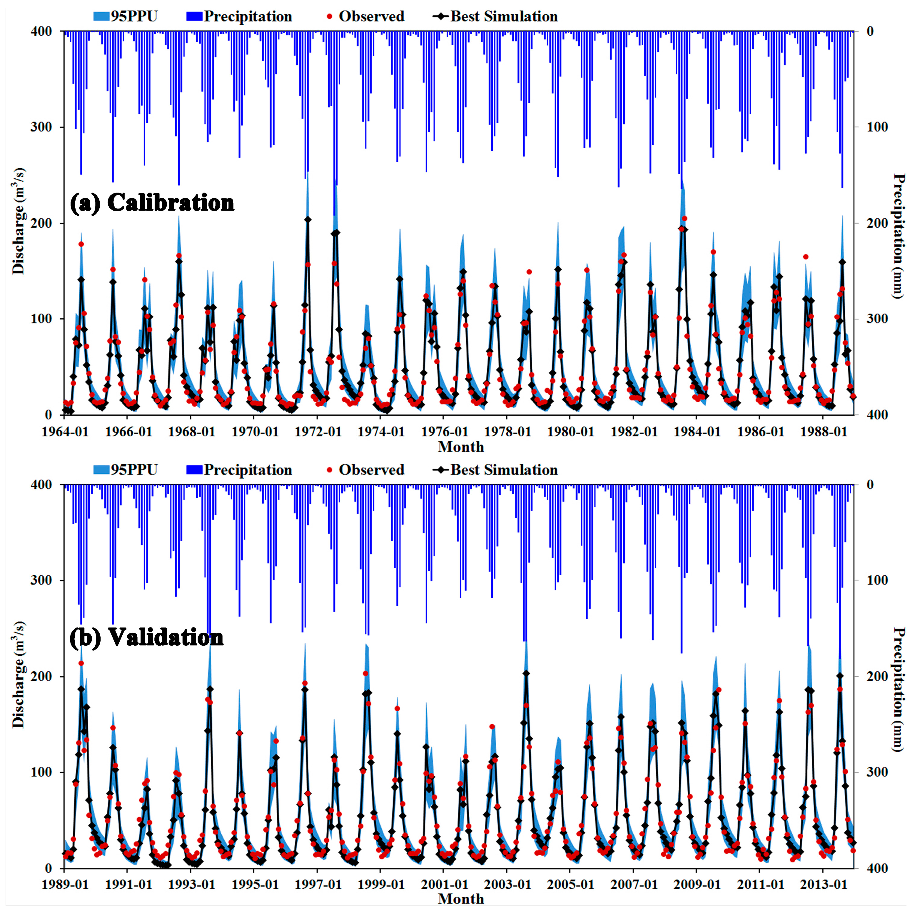
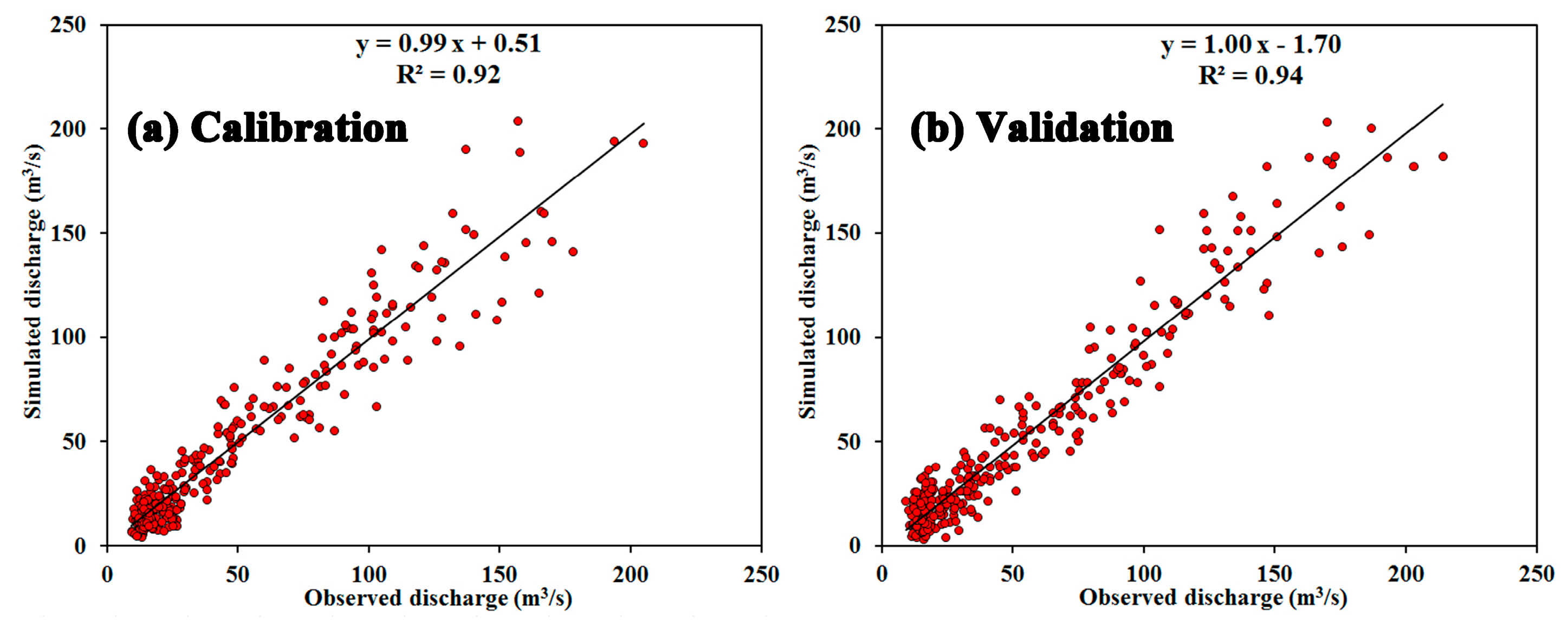
3.1. Model Performance

The model performance was shown in

Table 3. Model performance based on monthly river discharge.

Period	NSE	R2	PBIAS (%)
Calibration (1964–1988)	0.91	0.92	−4.5
Validation (1989–2013)	0.92	0.94	−6.8
The whole period (1964–2013)	0.92	0.93	−5.3

and Figure 3. We considered that SWAT simulated the observed monthly river discharge series fairly through NSE at 0.91 and 0.92 of the YLX hydrological station during calibration and validation periods, respectively. The high NSE values demonstrated that the results of model simulation met ‘very good performance’ according to the performance classification of Moriasi et al. [39]. Moreover, the values of R² in the two periods showed that the simulated results had a high correlation with the observed data, as shown in Figure 4. The values of PBIAS indicated that the model slightly underestimated when compared to the observed data. However, these underestimations were still within a reasonable scope.

Moreover, the 95PPU model results are shown in Figure 3, wherein the uncertainty of the modeling is shown as the shaded region that includes most types of uncertainties in the model prediction. The result showed that the P-factor was 88% and R-factor was 0.76 in the calibration period and also showed the two performance criteria were quite satisfactory. This indicated that SWAT is indeed a robust tool in the upper stream of HRB with high performance accuracy.

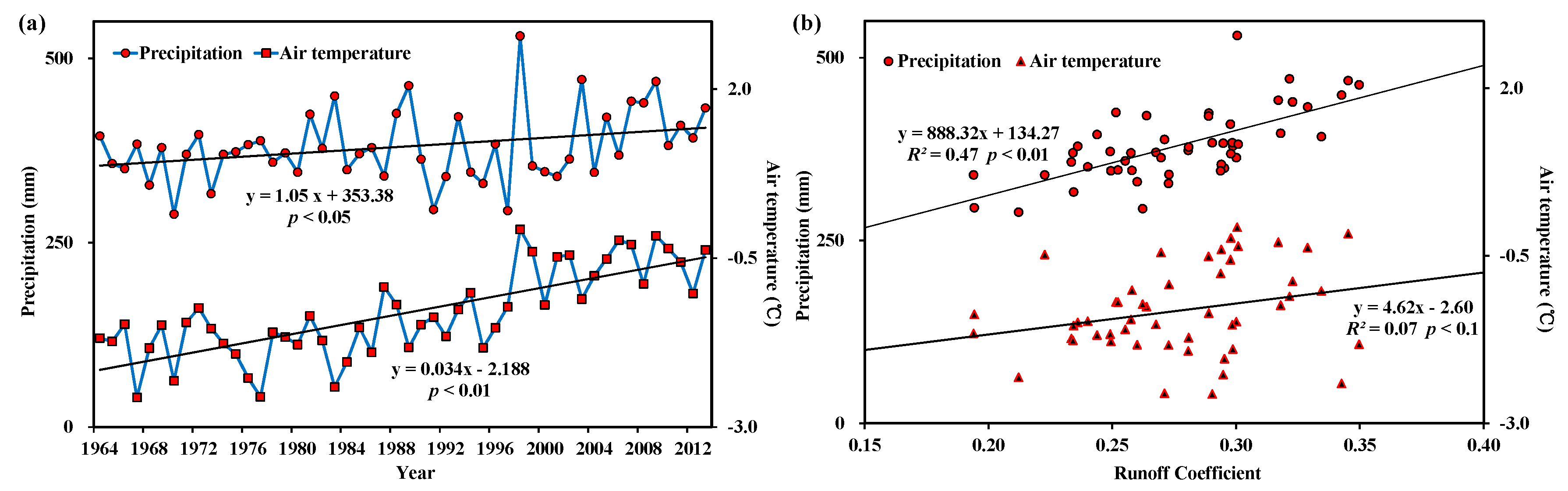
3.2. A Changing Trend in Water Balance Components at the Watershed Scale

In this paper, the water balance components we mentioned included the precipitation (P), the evapotranspiration (ET), the total runoff (Q), the surface runoff (Qs), the groundwater flow (Qg), and the soil water content (SW), wherein Q = Qs + Qg. The precipitation and air temperature data of the six meteorological stations were also used in the variation trends analysis. The annual variations of precipitation and air temperature were averaged by the data of TL, YNG, and QLX meteorological stations which were located in the deep of Qilian Mountain during 1964–2013 as shown in Figure 5a; the precipitation showed an upward trend, increasing at an average rate of 1.05 mm/a (significance level p < 0.05), and the annual average air temperature increased significantly by 0.034 °C/a (significance level p < 0.01). It indicated that climate change has impacted upon this region with more moisture and warming during last 50 years [40,41]. According to the relationship between the annual runoff coefficient (annual runoff/annual precipitation) with precipitation and air temperature (Figure 5b), we found that there was a relatively higher correlation between runoff coefficient and precipitation, compared to that of air temperature. This indicated that precipitation is the major factor that influences the increase of streamflow in the YLX watershed. The impact of the air temperature on streamflow was non-significant.

Over the past 50 years, the annual average precipitation and total runoff of the watershed have increased with climate change, with an increasing trend of 5.8 mm/10a and 8.2 mm/10a, respectively. According to the calculation results, the ET of the watershed accounted for 70.9% of the precipitation. The surface runoff and groundwater flow changes remained consistent with the total runoff, showing an increasing trend with the rates of 3.5 mm/10a and 4.7 mm/10a, respectively. The annual average contribution of surface runoff and groundwater flow to total runoff were 67.1% and 32.9%, respectively. However, the contribution rate of surface runoff and groundwater flow for the total runoff increase were 42.7% and 57.3%, respectively. This meant that the contribution of the increasing of groundwater flow to the increase of total runoff was larger than the increase of surface runoff. The change trend of soil water content kept relatively stable, with a rising trend of only 1.2 mm/10a.

3.3. Quantification of Water Balance Components at the Landscape Scale

The composition ratio and area percentage of water balance components at landscape scale are shown in Figure 6a. The alpine meadow occupied the largest area (51.1% of the watershed), and, as a consequence, accounted for the largest portion of each water balance component. The runoff generated from the alpine meadow contributed 55.5% to the total runoff of the watershed, with 31.9% from the surface runoff and 23.6% from the groundwater flow, respectively. The runoff coefficient of the alpine meadow was 0.33 (shown in Figure 6b) which equals to the runoff coefficient of the whole watershed. Considering the runoff contribution, runoff coefficient, and the area percentage, we could see that the alpine meadow was the most important vegetation type in the YLX watershed. Grassland accounted for 14.2% of the study area, which could lead to canopy interception and the capability of regulation and storage at the root zone; the water-yielding capacity was low with the lowest runoff coefficient which was 0.24. ET from the grassland landscape accounted for 16.0% of that in the whole watershed, while the groundwater flow from the grassland only accounted for 4.7% of the total groundwater flow of the watershed, which indicated that there was little extra water infiltrating into the underground. The runoff generated from the bare land (15.4% of the watershed) contributed 15.9% to the total runoff of the watershed, with 12.6% from the surface runoff and only 3.3% from the groundwater flow. The ET and soil water content formed in the bare land were relatively low, contributing 8.4% and 7.5% of the total ET and soil water content of the watershed, respectively. Because the bare land mainly is composed by alpine cold desert, which was in a cold environment, the soil of the alpine cold desert was thinner, and was unable to hold more soil moisture. So, the runoff coefficient of the bare land was relatively higher, equaling 0.46. There was an argument in the mountainous area of the inland river basin in semi-arid and arid regions that was whether the forest could generate runoff. In this study, the forest land included a large portion of shrub, so there was 16.9% of the total runoff of the watershed generated from the forest land (forest and shrub, 18.8% of the watershed) with 12.4% from the surface runoff and 4.5% from the groundwater flow. The runoff coefficient of the forest land was 0.32 as shown in the Figure 6b. The runoff coefficient of the glacier was 0.87; however, because the area percentage was very small, the contribution only occupied 3.2% of total runoff.

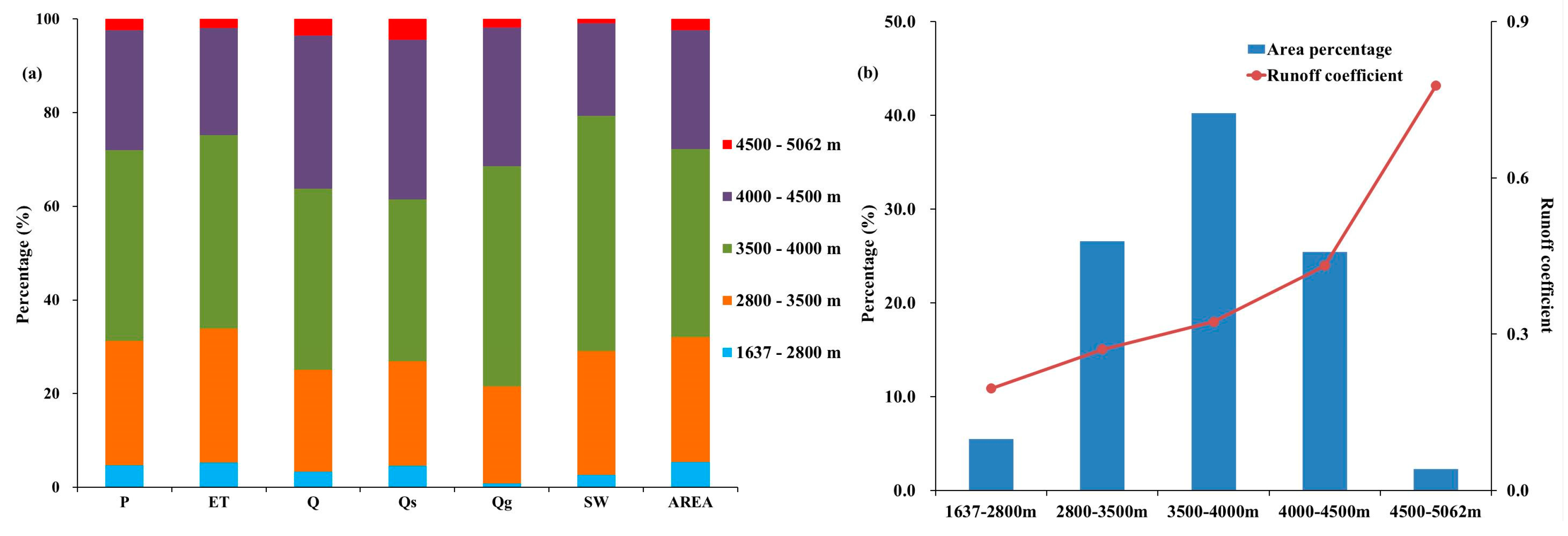
3.4. Quantification of Water Balance Components and Changing Trends across Elevation Zones

Water balance analysis at different elevations zones is of critical importance for understanding the water balance of an alpine mountainous area in an inland river basin. Based on the vertical gradient of the landscape and the elevation, five elevation zones were divided in this paper, including zones of: 1637 to 2800 m, 2800 to 3500 m, 3500 to 4000 m, 4000 to 4500 m, and 4500 to 5062 m.

The composition ratio and area percentage of water balance components at the elevation zone scale was demonstrated in Figure 7a. The zone of 3500 to 4000 m had the largest area (40.2% of the watershed), and meanwhile, accounted for the largest portion of each water balance component. The runoff generated from this elevation zone contributed 38.7% of the total runoff of the watershed with 23.2% from surface runoff and 15.5% from the groundwater flow. The runoff coefficient of this zone was 0.32 (shown in the Figure 7b) which was close to the runoff coefficient of the whole watershed (0.33). The zones of 1637 to 2800 m, 2800 to 3500 m, 4000 to 4500 m, and 4500 to 5062 m covered 5.5%, 26.6%, 25.4%, and 2.3% of the watershed, and contributed 2.6%, 21.7%, 32.0, and 5.1% of the total runoff, respectively. We could see that the zone of 3500 to 4500 m occupied a great part of the watershed area (65.6%), and contributed most of the total runoff (70.7%). The zone of 4500 to 5062 m was mainly covered by snow and glacier, and the zone of 1637 to 2800 m was the arid steppe zone and the portion of each water balance component in these two zones was lower than 5% as shown in Figure 7a. However, because of the melting water of the glacier and snow in zone of 4500 to 5062 m, the runoff coefficient was the highest with the value of 0.78. The zone of 4000 to 4500 m was located in a cold and humid environment, which means the proportions of ET and soil water content were relatively low. The dominant runoff component was surface runoff, with a relatively higher runoff coefficient (0.43). The zone of 2800 to 3500 m was warm and dry, covered by thick soil. The precipitation in this zone was primarily consumed by evapotranspiration and stored in the soil gaps as soil water, so the runoff coefficient was low (0.27). The zone of 1637 to 2800 m was in a drier and warmer environment, so there was little runoff generated with the runoff coefficient was 0.20. Wang et al. [42] used the stable isotope technique to trace the major source area of the mountainous runoff generation of the Heihe River and realized that the mountainous runoff was generated mostly at high altitudes. They revealed that 80.2% of the annual total mountainous runoff amount was generated at the area above 3600 m. The results indicated that we should pay much more attention to the impact of climate change in the high altitudes on the water balance components in mountainous watersheds of inland river basins.

The changing trends in water balance components for different elevation zones were shown in

Table 4. The change trend of water balance components for different elevation zones during 1964 to 2013 (unit: mm/10a).

Elevation Zone/m	Precipitation	ET	Runoff	Surface Runoff	Groundwater Flow	Soil Water Content
1637–2800	5.0	−2.0	7.1 **	5.3 **	1.8 **	3.8 **
2800–3500	4.3	−3.4	7.9 **	3.4 **	4.5 **	2.4 *
3500–4000	5.8	−3.4	8.8 **	3.1 *	5.7 **	0.8
4000–4500	7.4	−1.2	8.1 **	3.6	4.5 **	0.0
4500–5062	7.8	0.5	6.9 *	4.6	2.3 **	−0.8

Notes: * represents the significance at level of 0.1; ** represents the significance at level of 0.05.

. The runoff from the five elevation zones were all having an increasing trend with the largest (smallest) value was 8.8 mm/10a (6.9 mm/10a) in the elevation zone of 3500 to 4000 m (4500 to 5062 m), and that all of the runoff change trends were statistically significant. So, the total runoff change trend at the watershed scale was 8.2 mm/10a. The surface runoff and groundwater flow from the five elevation zones were all increasing during the last 50 years, and the groundwater flow was more obvious, indicated by the results at the elevation zone scale. Therefore, the increasing rate of groundwater flow was larger than that of the surface runoff at the watershed scale with the value of 4.7 mm/10a and 3.5 mm/10a, respectively. The trends in precipitation change at the elevation zone scale were all positive. There was a phenomenon that increasing rates were larger as elevation increased. However, a change in the trend of precipitation at the elevation zone scale was not significant.

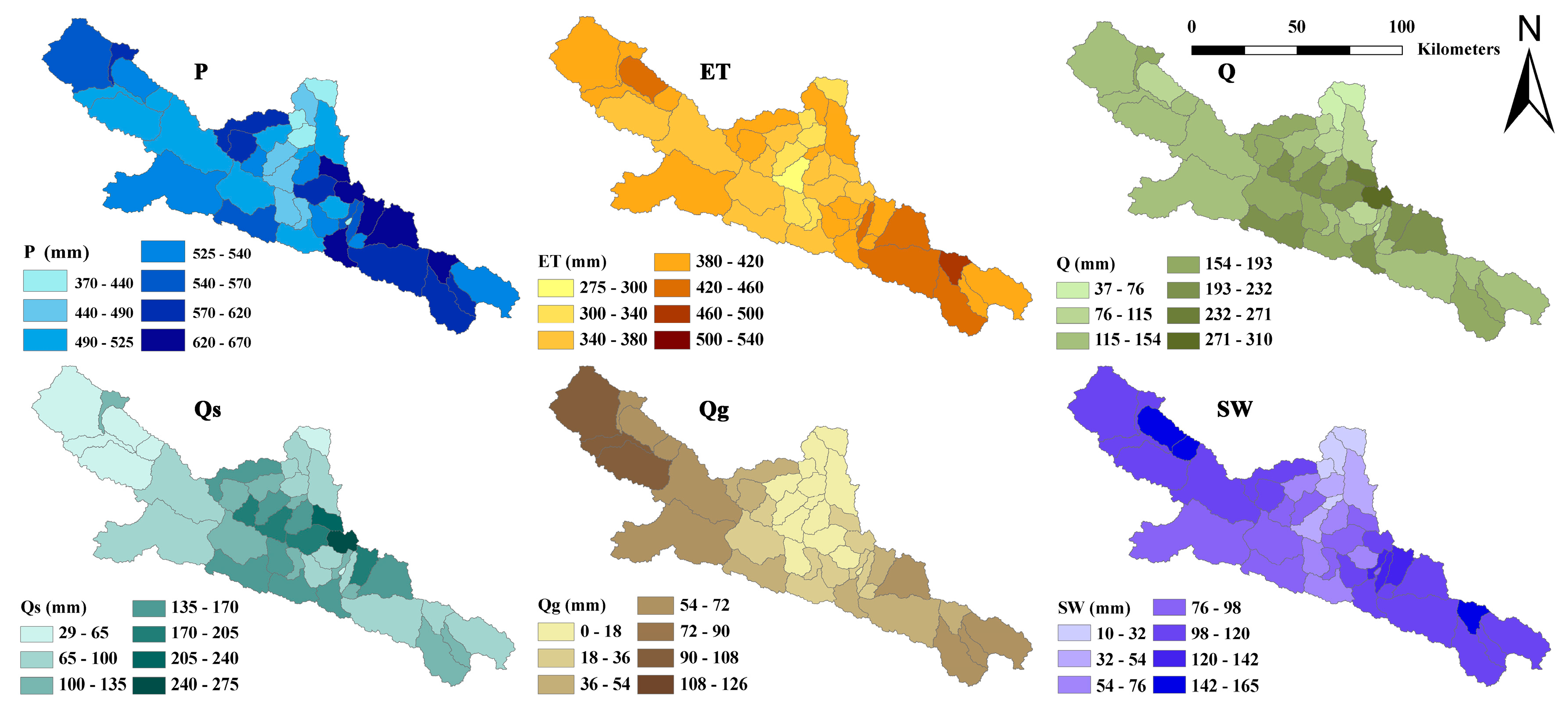
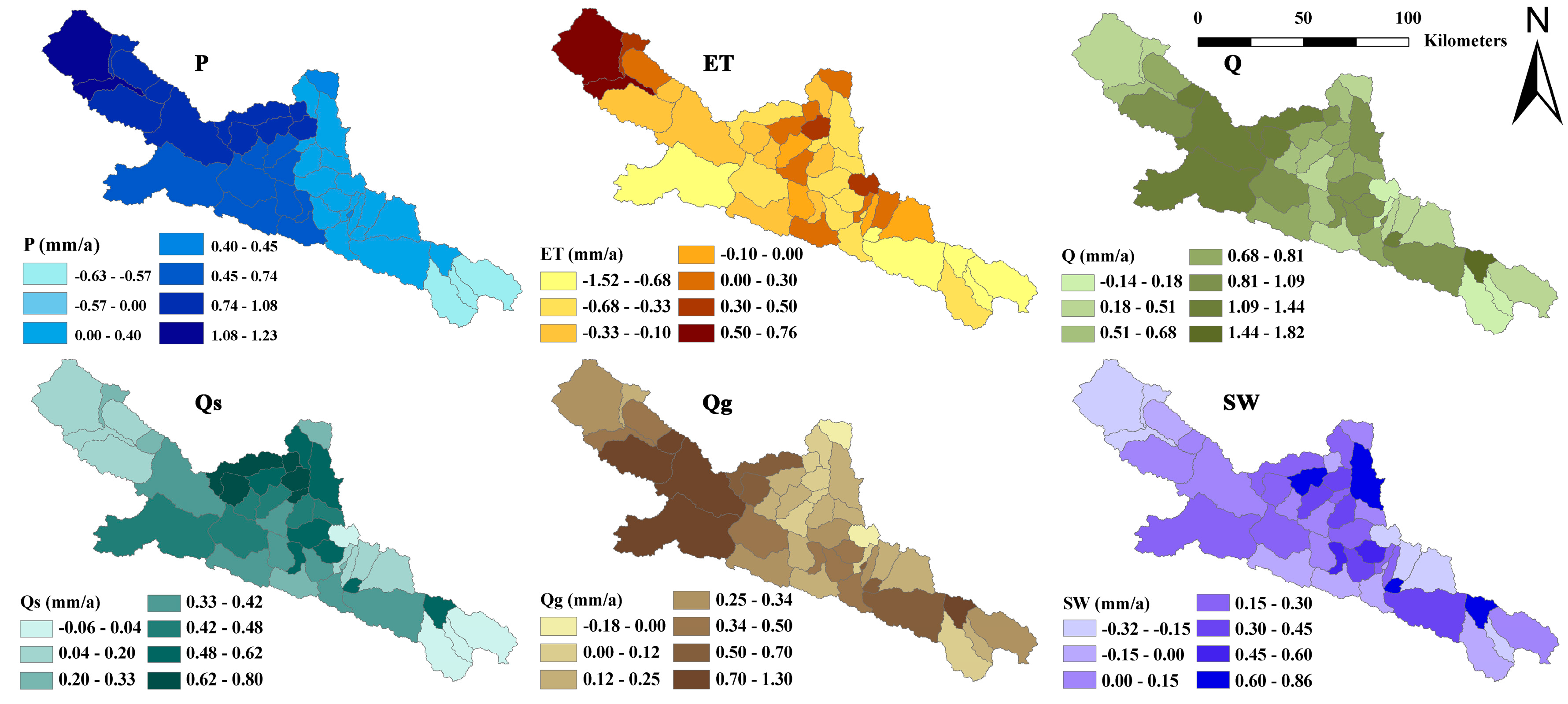
3.5. Quantification of Water Balance Components and the Change Trends at the Sub-Watershed Scale

The annual average values of water balance components at the sub-watershed scale were different as shown in Figure 8. The annual average precipitation varied from 370 to 670 mm at the sub-watershed scale, decreasing from east to west on the space. The annual average precipitation was larger in the eastern sub-watersheds than that of the western sub-watersheds. The annual average sub-watershed ET varied from 275 to 540 mm with the ET of 384.2 mm at the watershed scale, as shown in Figure 8. The total runoff varied tremendously at the sub-watershed scale with the annual average value from 37 mm to 310 mm (the annual average value was 151.5 mm during 1964 to 2013 at the watershed scale) demonstrating that the sub-watersheds had different water yield capacity because of the different underlying surface. The spatial distribution pattern of the surface runoff was similar with that of the total runoff, which was larger in the central sub-watersheds and smaller in the east and west. The annual average sub-watershed surface runoff varied from 29 mm to 275 mm (101.6 mm at the watershed scale), as shown in Figure 8. The spatial distribution pattern of the groundwater flow was opposite to that of the surface runoff, showing that there was little ground water (the annual average value was smaller than 18 mm) flowing into the river in the central sub-watersheds and a considerable amount of ground water feeding the river in the western and eastern sub-watersheds with the largest value of 126 mm in the most western sub-watershed. The annual average groundwater flow of the whole watershed was 49.9 mm according to the summation of the sub-watershed scale results. The annual average soil water content varied from 10 mm to 165 mm at the sub-watershed scale (96.9 mm at the watershed scale), as shown in Figure 8.

Trends in the change of water balance components at the sub-watershed scale were shown in Figure 9. The increasing rate of the precipitation reduced from west to east, with the largest value of 1.23 mm/a in the most western sub-watershed. Only the three most eastern sub-watersheds’ precipitation were decreasing during the past 50 years, and the precipitation of the other 40 sub-watersheds were increasing, which lead to an increasing rate of 5.8 mm/10a at the watershed scale. The change trend of ET at the sub-watershed scale varied between −1.52 and 0.76 mm/a. All except one runoff of sub-watersheds had increasing trend from 0.18 mm/a to 1.81 mm/a. Consequently, the total runoff at the watershed scale presented an increasing trend of 8.2 mm/10a. The increasing rate of the total runoff in the west part of the watershed was more significant compared to that of the central and eastern regions. Trends in the sub-watershed surface runoff varied from −0.06 to 0.80 mm/a. There was only one sub-watershed having a decreasing surface runoff with the trend of −0.06 mm/a, the others had an increasing trend. The change trend of the surface runoff at the whole watershed was 3.5 mm/10a during 1964 to 2013. The spatial distribution of the change trend of groundwater flow was very similar to that of the total runoff at the sub-watershed scale. The range of the change trend of the sub-watershed groundwater flow was −0.18 to 1.30 mm/a. Similarly, the change trend of groundwater flow of the whole watershed was increasing with the value of 4.7 mm/10a, based on the results of the sub-watershed scale. The change trend of soil water content at the sub-watershed scale varied between −0.32 and 0.86 mm/a (1.2 mm/10a at the watershed scale), respectively, as shown in Figure 9.

4. Discussion

Mountainous watersheds are the main water generating regions in inland river basins. Better understanding of the variation characteristics and the spatial distribution of the water balance components experiencing climate change is crucial for sustainable water resource management in semi-arid and arid inland river basins [43,44,45,46]. Previous studies have facilitated our current understanding at specific scales. However, the multi-scales analysis is necessary to fully understand the interaction between the hydrological processes and environment. This study provided insights into quantities and change trends of the water balance components for the water resource region at different spatial scales (watershed scale, landscape scale, elevation zone scale, and sub-watershed scale), taking the upper reaches of the Heihe River Basin as a case. From the results, we could fill in the multi-scale knowledge gap of water balance of the mountainous watershed in inland river basins. This information is very useful for developing an overview of where the water resources are coming from and what changes have been taken place during the past half century. This study will provide a theoretical reference for the water resources management of the inland river basins of China [47,48].

There are several limitations in this study. First, the lack of field observation data—for example, soil moisture and actual evapotranspiration—hampers the validation of the simulation. Each landscape has different impacts on the hydrological process and in mountains, the water balance components vary in different landscapes [22]. Moreover, spatial heterogeneity of soil has great impact on the dynamic processes of hydrological systems. The lack of observational data will influence the simulation accuracy. Second, we neglect the impact of human activities, the change trends of water balance components are completely related to climatic factors such as precipitation and temperature. Although several studies have shown that the climate variability is mainly influenced the hydrological processes in mountainous watersheds of the inland river basins [29,41,48,49,50], somehow human activities will have some influence on the water cycle. Third, the SWAT model does not incorporate the soil freezing/thawing processes. The study area is located in a mountainous region within which there is distributed a wide range of permafrost and seasonally cold regions. The soil freezing/thawing processes will influence the simulation accuracy [27].

References

1. Eder, G.; Fuchs, M.; Nachtnebel, H.P.; Loibl, W. Semi-distributed modeling of the monthly water balance in an alpine catchment. Hydrol. Process. 2005, 19, 2339–2360. [Google Scholar] [CrossRef]
2. Wang, W.; Peng, S.; Yang, T.; Shao, Q.; Xu, J.; Xing, W. Spatial and temporal characteristics of reference evapotranspiration trends in the Haihe River Basin, China. J. Hydrol. Eng. 2011, 16, 239–252. [Google Scholar] [CrossRef]
3. Gunkel, A.; Shadeed, S.; Hartmann, A.; Wagener, T.; Lange, J. Model signatures and aridity indices enhance the accuracy of water balance estimation in a data-scarce Eastern Mediterranean catchment. J. Hydrol. Reg. Stud. 2015, 4, 487–501. [Google Scholar] [CrossRef]
4. Wang, N.L.; Wu, H.B.; Wu, Y.W.; Chen, A.A. Variations of the glacier mass balance and lake water storage in the Tarim Basin, northwest China, over the period of 2003–2009 estimated by the ICESatGLAS data. Environ. Earth Sci. 2015, 74, 1997–2008. [Google Scholar] [CrossRef]
5. Fujieda, M.; Kudoh, T.; Cicco, V.; Calvarcho, J.L. Hydrological processes at two subtropical forest catchments: The Serra do Mar, São Paulo, Brazil. J. Hydrol. 1997, 196, 26–46. [Google Scholar] [CrossRef]
6. Fiseha, B.M.; Setegn, S.G.; Melesse, A.M.; Volpi, E.; Fiori, A. Hydrological analysis of the Upper Tiber River Basin, Central Italy: A watershed modeling approach. Hydrol. Process. 2013, 27, 2339–2351. [Google Scholar] [CrossRef]
7. Ngongondo, C.; Xu, C.Y.; Tallaksen, L.M.; Alemaw, B. Observed and simulated changes in the water balance components over Malawi, during 1971–2000. Quatern. Int. 2015, 369, 7–16. [Google Scholar] [CrossRef]
8. Ning, J.C.; Gao, Z.Q.; Lu, Q.S. Runoff simulation using a modified SWAT model with spatially continuous HRUs. Environ. Earth Sci. 2015, 74, 5895–5905. [Google Scholar] [CrossRef]
9. Lu, Z.X.; Zou, S.B.; Xiao, H.L.; Zheng, C.M.; Yin, Z.L.; Wang, W.H. Comprehensive hydrologic calibration of SWAT and water balance analysis in mountainous watersheds in northwest China. Phys. Chem. Earth 2015, 79–82, 76–85. [Google Scholar] [CrossRef]
10. Arnold, J.G.; Srinivasan, R.; Muttiah, R.S.; Allen, P.M. Continental scale simulation of the hydrologic balance. J. Am. Water Resour. Assoc. 1999, 35, 1037–1051. [Google Scholar] [CrossRef]
11. Jiang, R.; Li, Y.; Wang, Q.; Kuramochi, K.; Hayakawa, A.; Woli, K.P.; Hatano, R. Modeling the water balance processes for understanding the components of river discharge in a Non-conservative Watershed. Tran. ASABE 2011, 54, 2171–2180. [Google Scholar] [CrossRef]
12. Fang, G.H.; Yang, J.; Chen, Y.N.; Xu, C.C.; Maeyer, P.D. Contribution of meteorological input in calibrating a distributed hydrologic model in a watershed in the Tianshan Mountains, China. Environ. Earth Sci. 2015, 74, 2413–2424. [Google Scholar] [CrossRef]
13. Kling, H.; Nachtnebel, H.P. A spatio-temporal comparison of water balance modeling in an Alpine catchment. Hydrol. Process. 2009, 23, 997–1009. [Google Scholar] [CrossRef]
14. Zhang, Y.Y.; Zhang, S.F.; Xia, J.; Hua, D. Temporal and spatial variation of the main water balance components in the three rivers source region, China from 1960 to 2000. Environ. Earth Sci. 2013, 68, 973–983. [Google Scholar] [CrossRef]
15. Gregory, J.M.; David, M.W. Temporal and spatial variability of the global water balance. Clim. Chang. 2013, 120, 375–387. [Google Scholar]
16. Herrmann, F.; Keller, L.; Kunkel, R.; Vereechen, H.; Wendland, F. Determination of spatially differentiated water balance components including groundwater recharge on the Federal State level—A case study using the mGROWA model in North Rhine-Westphalia (Germany). J. Hydrol. Reg. Stud. 2015, 4, 294–312. [Google Scholar] [CrossRef]
17. White, E.D.; Easton, Z.M.; Fuka, D.R.; Collick, A.S.; Adgo, E.; McCartney, M.; Awulachew, S.B.; Selassie, Y.G.; Steenhuis, T.S. Development and application of a physically based landscape water balance in the SWAT model. Hydrol. Process. 2011, 25, 915–925. [Google Scholar] [CrossRef]
18. Uniyal, B.; Jha, M.K.; Verma, A.K. Assessing climate change impact on water balance components of a river basin using SWAT model. Hydrol. Process. 2015, 29, 4767–4785. [Google Scholar] [CrossRef]
19. Jian, S.Q.; Zhao, C.Y.; Fang, S.M.; Yu, K. Effects of different vegetation restoration on soil water storage and water balance in the Chinese Loess Plateau. Agric. For. Meteorol. 2015, 206, 85–96. [Google Scholar] [CrossRef]
20. Thompson, S.E.; Harman, C.J.; Troch, P.A.; Brooks, P.D.; Sivapalan, M. Spatial scale dependence of ecohydrologically mediated water balance partitioning: A systhesis framework for catchment ecohydrology. Water Resour. Res. 2011, 47, 143–158. [Google Scholar] [CrossRef]
21. Knowles, J.F.; Harpold, A.A.; Cowie, R.; Zeliff, M.; Barnard, H.R.; Burns, S.P.; Blanken, P.D.; Morse, J.F.; Williams, M.W. The relative contributions of alpine and subalpine ecosystems to the water balance of a mountainous, headwater catchment. Hydrol. Process. 2015, 29, 4794–4808. [Google Scholar] [CrossRef]
22. Qin, J.; Ding, Y.J.; Wu, J.K.; Gao, M.J.; Yi, S.H.; Zhao, C.C.; Ye, B.S.; Li, M.; Wang, S.X. Understanding the impact of mountain landscapes on water balance in the upper Heihe River watershed in northwestern China. J. Arid Land 2013, 5, 366–383. [Google Scholar] [CrossRef]
23. Guo, J.; Su, X.L.; Singh, V.P.; Jin, J.M. Impacts of climate and land use/cover change on streamflow using SWAT and a separation method for the Xiying River Basin in Northwestern China. Water 2016, 8, 192. [Google Scholar] [CrossRef]
24. Li, Z.L.; Wang, Y.H.; Zhao, W.; Xu, Z.X.; Li, Z.J. Frequency analysis of high flow extremes in the Yingluoxia watershed in Northwest China. Water 2016, 8, 215. [Google Scholar] [CrossRef]
25. Zang, C.F.; Liu, J.G. Trend analysis for the flows of green and blue water in the Heihe River basin, northwestern China. J. Hydrol. 2013, 502, 27–36. [Google Scholar] [CrossRef]
26. Yin, Z.L.; Xiao, H.L.; Zou, S.B.; Zhu, R.; Lu, Z.X.; Lan, Y.C.; Shen, Y.P. Simulation of hydrological processes of mountainous watersheds in inland river basin: Taking the Heihe mainstream river as an example. J. Arid Land 2014, 6, 16–26. [Google Scholar] [CrossRef]
27. Yang, D.W.; Gao, B.; Jiao, Y.; Lei, H.M.; Zhang, Y.L.; Yang, H.B.; Cong, Z.T. A distributed scheme developed for eco-hydrological modeling in the upper Heihe River. Sci. China Earth Sci. 2015, 58, 36–45. [Google Scholar] [CrossRef]
28. Deng, X.Z.; Shi, Q.L.; Zhang, Q.; Shi, C.C.; Yin, F. Impacts of land use and land cover changes on surface energy and water balance in the Heihe River Basin of China, 2000–2010. Phys. Chem. Earth 2015, 79–82, 2–10. [Google Scholar] [CrossRef]
29. Wu, F.; Zhan, J.Y.; Wang, Z.; Zhang, Q. Streamflow variation due to glacier melting and climate change in upstream Heihe River Basin, Northwest China. Phys. Chem. Earth 2015, 79–82, 11–19. [Google Scholar] [CrossRef]
30. Wang, J.F.; Gao, Y.C.; Wang, S. Land use/cover change impacts on water table change over 25 years in a desert-oasis transition zone of the Heihe River Basin, China. Water 2016, 8, 11. [Google Scholar] [CrossRef]
31. Cheng, G.D.; Li, X.; Zhao, W.Z.; Xu, Z.M.; Feng, Q.; Xiao, S.C.; Xiao, H.L. Integrated study of the water-ecosystem-economy in the Heihe River Basin. Natl. Sci. Rev. 2014, 1, 413–428. [Google Scholar] [CrossRef]
32. Arnold, J.G.; Srinivasan, R.; Williams, J.R. Large area hydrologic modeling and assessment. Part I: Model development. J. Am. Water Resour. Assoc. 1998, 34, 73–89. [Google Scholar] [CrossRef]
33. Neitsch, S.L.; Arnold, J.G.; Kiniry, J.R.; Williams, J.R. Soil and Water Assessment Tool Theoretical Documentation: Version 2005; USDA-ARS Grassland, Soil and Water Research Laboratory: Temple, TX, USA, 2005. [Google Scholar]
34. Hock, R. Temperature index melt modeling in mountain areas. J. Hydrol. 2003, 282, 104–115. [Google Scholar] [CrossRef]
35. Rahman, K.; Maringanti, C.; Beniston, M.; Windmer, F.; Abbaspour, K.; Lehmann, A. Streamflow modeling in a highly managed mountainous glacier watershed using SWAT: The upper Rhone River watershed case in Switzerland. Water Resour. Manag. 2013, 27, 323–339. [Google Scholar] [CrossRef]
36. Saxton, K.E.; Rawls, W.J. Soil water characteristic estimates by texture and organic matter for hydrologic solutions. Soil Sci. Soc. Am. J. 2006, 70, 1569–1578. [Google Scholar] [CrossRef]
37. Skaggs, T.H.; Arya, L.M.; Shouse, P.J.; Mohanty, B.P. Estimating particle-size distribution from limited soil texture data. Soil Sci. Soc. Am. J. 2001, 65, 1038–1044. [Google Scholar] [CrossRef]
38. Abbaspour, K.C. SWAT-CUP, SWAT Calibration and Uncertainty Programs; Swiss Federal Institute of Aquatic Science and Technology: Dübendorf, Switzerland, 2011. [Google Scholar]
39. Moriasi, D.; Arnold, J.G.; Van Liew, M.W.; Bingner, R.; Harmel, R.; Veith, T.L. Model evaluation guidelines for systematic quantification of accuracy in watershed simulations. Trans. ASABE 2007, 50, 885–900. [Google Scholar] [CrossRef]
40. Shi, Y.F.; Shen, Y.P.; Hu, R.J. Preliminary study on signal, impact and foreground of climatic shift from warm-dry to warm-humid in Northwest China. J. Glaciol. Geocryol. 2002, 24, 219–226. [Google Scholar]
41. Wang, J.; Meng, J. Characteristics and tendencies of annual runoff variations in the Heihe River Basin during the past 60 years. Sci. Geogr. Sin. 2008, 28, 83–88. [Google Scholar]
42. Wang, N.L.; Zhang, S.B.; He, J.Q.; Pu, J.C.; Wu, X.B.; Jiang, X. Tracing the major source area of the mountainous runoff generation of the Heihe River in northwest China using stable isotope technique. Chin. Sci. Bull. 2009, 54, 2751–2757. [Google Scholar] [CrossRef]
43. Li, Z.H.; Deng, X.Z.; Wu, F.; Hasan, S.S. Scenario analysis for water resources in response to land use change in the middle and upper reaches of the Heihe River Basin. Sustainability 2015, 7, 3086–3108. [Google Scholar] [CrossRef]
44. Nian, Y.Y.; Li, X.; Zhou, J.; Hu, X.L. Impact of land use change on water resource allocation in the middle reaches of the Heihe River Basin in northwestern China. J. Arid Land 2014, 6, 273–286. [Google Scholar] [CrossRef]
45. Ji, X.B.; Kang, E.S.; Chen, R.S.; Zhao, W.Z.; Xiao, S.C.; Jin, B.W. Analysis of water resources supply and demand and security of water resources development in irrigation regions of the middle reaches of the Heihe River Basin, Northwest China. Agric. Sci. China 2006, 5, 130–140. [Google Scholar] [CrossRef]
46. Du, C.; Sun, F.; Yu, J.; Liu, X.; Chen, Y. New interpretation of the role of water balance in an extended Budyko hypothesis in arid regions. Hydrol. Earth Syst. Sci. 2016, 20, 393–409. [Google Scholar] [CrossRef]
47. Zeng, Z.; Liu, J.; Koeneman, P.H.; Zarate, E.; Hoekstra, A.Y. Assessing water footprint at river basin level: A case study for the Heihe River Basin in northwest China. Hydrol. Earth Syst. Sci. 2012, 16, 2771–2781. [Google Scholar] [CrossRef]
48. Zang, C.; Liu, J.; Jiang, L.; Gerten, D. Impacts of human activities and climate variability on green and blue water flows in the Heihe River Basin in Northwest China. Hydrol. Earth Syst. Sci. Disscuss. 2013, 10, 9477–9504. [Google Scholar] [CrossRef]
49. Wu, F.; Zhan, J.Y.; Su, H.B.; Yan, H.M.; Ma, E.J. Scenario-based impact assessment of land use/cover and climate changes on watershed hydrology in Heihe River Basin of Northwest China. Adv. Meteorol. 2015, 2015, 410198. [Google Scholar] [CrossRef]
50. Zhang, L.; Nan, Z.T.; Yu, W.J.; Ge, Y.C. Modeling land-use and land-cover change and hydrological responses under consistent climate change scenarios in the Heihe River Basin, China. Water Resour. Manag. 2015, 29, 4701–4717. [Google Scholar] [CrossRef]
Figure 1. The study area, meteorological and hydrological stations in the YLX watershed.
Water 08 00472 g001
Figure 2. Two periods of vegetation map (left: version 1.0; right: version 2.0).
Water 08 00472 g002
Figure 3. Monthly river discharge of the YLX hydrological station during the calibration period (a); and the validation period (b); the uncertainties of simulation (95PPU); and the monthly precipitation of the YLX watershed.
Water 08 00472 g003
Figure 4. Correlation between the observed and simulated monthly river discharge of the YLX hydrological station during the calibration period (a) and the validation period (b).
Water 08 00472 g004
Figure 5. The change trend of precipitation and air temperature (a); and the correlation of runoff coefficient and precipitation and air temperature (b); from 1964 to 2013.
Water 08 00472 g005
Figure 6. The percentage of the water balance components and area (a); and the runoff coefficient (b); at the landscape scale.
Water 08 00472 g006
Figure 7. The percentage of the water balance components and area (a); and the runoff coefficient (b); at the elevation zone scale.
Water 08 00472 g007
Figure 8. The annual average value of water balances components at the sub-watershed scale.
Water 08 00472 g008
Figure 9. The change trend of water balances components at the sub-watershed scale during 1964 to 2013.
Water 08 00472 g009