Assessing Uncertainties of Water Footprints Using an Ensemble of Crop Growth Models on Winter Wheat

Abstract

Crop productivity and water consumption form the basis to calculate the water footprint (WF) of a specific crop. Under current climate conditions, calculated evapotranspiration is related to observed crop yields to calculate WF. The assessment of WF under future climate conditions requires the simulation of crop yields adding further uncertainty. To assess the uncertainty of model based assessments of WF, an ensemble of crop models was applied to data from five field experiments across Europe. Only limited data were provided for a rough calibration, which corresponds to a typical situation for regional assessments, where data availability is limited. Up to eight models were applied for wheat. The coefficient of variation for the simulated actual evapotranspiration between models was in the range of 13%–19%, which was higher than the inter-annual variability. Simulated yields showed a higher variability between models in the range of 17%–39%. Models responded differently to elevated CO₂ in a FACE (Free-Air Carbon Dioxide Enrichment) experiment, especially regarding the reduction of water consumption. The variability of calculated WF between models was in the range of 15%–49%. Yield predictions contributed more to this variance than the estimation of water consumption. Transpiration accounts on average for 51%–68% of the total actual evapotranspiration.

1. Introduction

The concept “Water Footprint” (WF) was introduced by [1], and later elaborated on by [2] as an indicator that relates human consumption to global water resources. Since international trade in commodities creates flows of so-called “virtual water” [2,3,4], by importing and exporting goods that require water for their production, the indicator provides valuable information for a global assessment of how water resources are used, although it was controversially discussed since water scarcity of the region is not accounted explicitly [5]. In recent years, WFs and virtual water was assessed for crops, goods, services, as well as on generic regional or national levels [2,4,6,7,8,9].

The Water Footprint (WF) of a crop is defined as the volume of water consumed for its production, where green and blue WF stand for rainfed and irrigation water usage, respectively [9]. A third component, the grey water footprint, is defined as the volume of freshwater that is required to dilute the load of pollutants to achieve existing ambient water quality standards. More information about the parameters involved can be found in [10].

Crop productivity and water consumption together form the basis to estimate the water footprint of a specific crop. The WF calculation is based on the estimation of crop specific evapotranspiration during the growing season, which is related to observed crop yields usually from yield statistics of a region. Analyses of several ET formulas under various climate conditions [11,12], revealed that the FAO (Food and Agriculture Organization of the United Nations) Penman–Monteith equation [13] or the Priestley–Taylor formula had the best performance across the different climatic conditions [12,14]. FAO Penman–Monteith is recommended as the standard method for estimating reference and crop evapotranspiration in the water footprint manual to estimate the water footprint [15].

Agricultural production systems are very vulnerable to a potential decrease in water availability. The impacts of climate change (increasing temperatures, shifts of seasonal precipitation and decreasing summer rainfall) could cause water limitations in many areas of Europe [16,17]. A change of currently estimated water footprint values is expected under climate change. However, it is not clear how far the above-mentioned negative impacts of a changing climate can be compensated by the positive effects of increasing CO₂. Climate change including increasing CO₂ concentration of the atmosphere will affect crop growth as well as soil water dynamics. Moreover, crop response to climatic drivers strongly depends on the site conditions of their habitat [18,19,20]. Therefore, the assessment of WF under future climate conditions requires the simulation of crop yields as well, which may add further uncertainty in the estimate.

Uncertainty may originate from three sources [21]: (i) input data; (ii) parameterization; and (iii) model structure. While uncertainty analyses of models addressing the first point are usually using combinations of stochastically distributed inputs by using, e.g., Monte-Carlo simulations (e.g., [22]), for the other two aspects recent studies have shown that the application of ensembles of complex simulation models is a valuable tool to assess the uncertainty in the estimation of climate impact on crop growth [23,24,25,26,27] and water consumption [28]. To assess the uncertainty of model based assessments of WF an ensemble of different crop models was applied to field data sets from five locations from across Europe. The focus of the study was mainly to look at uncertainty originating from the use of different models. Only limited basic data were made available to allow only a rough calibration, which corresponds to a typical situation for regional assessments, where data availability is limited. Although a separation between the uncertainty resulting from model structures and parameter uncertainty is not possible with this approach, the basic data provided in this study for each experimental site contained defined values for field capacity and wilting point and key phenological observations to keep the uncertainty caused by soil and crop parameterization at a limited level. Up to eight models were applied depending on the data set. In the comparison, we focused on cereal crops, mainly winter wheat. The objective of the study was to: (1) assess the uncertainty of the WF estimation caused by the choice of crop models; (2) analyze the response of models to management (irrigation, nitrogen fertilization) and site conditions (soils, CO₂ concentration of the atmosphere); and (3) separate soil evaporation from crop transpiration to assess the difference of using evapotranspiration instead of crop transpiration for the crop water consumption assessment.

2. Materials and Methods

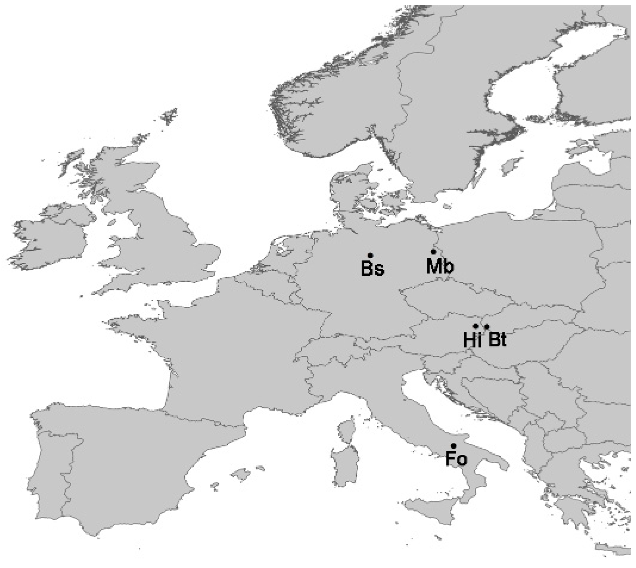
2.1. Experimental Data

The five datasets cover the European environmental zones of the Atlantic North, Atlantic Central, Continental and Pannonia according to [29] (Figure 1). The criteria to select data sets were that they provide: (a) meteorological and management data for several years; (b) different treatments or site conditions to analyze crop sensitivity on different inputs; and (c) data to evaluate the relevant outputs for the estimation of the water footprint, particularly crop yield and soil water (and if possible soil mineral nitrogen) status measurements. The basic characteristics of the experimental sites and the treatments used for the model inter-comparison are listed in

Table 1. Characterization of experimental data.

Location/Country	Topography	Period	Climate *	Soil # S/Si/Cl/Corg	Treatment	Crops
Müncheberg/Germany	Lat: 52.52° Long: 14.12° Elev: 62 m a.s.l.	1992–1998	8.4 °C 563 mm	83/9/8/0.6	shifted rotation, rainfed, irrigated	sugar beet, winter wheat, winter barley, winter rye (oil raddish)
Braunschweig/Germany	Lat: 52.3° Long: 10.45° Elev: 79 m a.s.l.	1999–2005	10.0 °C 642 mm	69/24/7/1.0	374/550 ppm CO2 2 nitrogen levels	winter barley, ryegrass (catchcrop), sugar beet, winter wheat
Hirschstetten/Austria	Lat: 48.2° Long: 16.57° Elev: 150 m a.s.l.	1998–2003	10.9 °C 495 mm	1: 22/50/28/2.9 2: 68/19/13/1.3 3: 22/54/24/1.3	3 soils	grain maize, winter wheat, spring barley, mustard , spring wheat, potatoes
Foggia/Italy	Lat: 41.26° Long: 15.30° Elev: 90 m a.s.l.	1995–2005	15.9 °C 540 mm	13/39/48/1.5	Straw burned Straw remained with 0, 50, 100 and 150 kg N/ha	Durum wheat
Bratislava/Slovakia	Lat: 48.16° Long: 17.23° Elev: 130 m a.s.l.	1998–2006	10.7 °C 575 mm	19/59/22/1.7	Rainfed, irrigated 2 nitrogen levels (0% and 100%) Residue management	w. wheat, maize, maize, maize, spr. barley, w. wheat, maize, spr. barley

Notes: * Annual mean temperature and annual precipitation for the given period. # Sand (S), silt (Si), clay (Cl) and organic carbon (Corg) content (mass%) in the plough layer

.

Here some brief information for each site is presented:

The field experiment at Müncheberg (Mb), Germany was designed to study inter-annual variation in crop rotations, irrigation effects, and biomass development [30]. The crop rotation from 1992 to 1998, consisted sugar beet (Beta vulgaris L.), winter wheat (Triticum aestivum L.), winter barley (Hordeum vulgare L.), winter rye (Secale cereale L.) and oilseed radish (catch crop). The rotation covered four parallel plots with a shift of one year to establish each crop each year. Treatments included rainfed agriculture versus irrigated regime. The complete dataset is published and accessible [31].

The Braunschweig (Bs) Free-Air Carbon Dioxide Enrichment (FACE) experiment was set up to investigate interacting effects of CO₂ concentration and N fertilization on crop production [32]. The crop rotation was composed of winter barley, a mixture of three different ryegrass cultivars (Lolium multiflorum Lam.) as a cover crop, sugar beet, and winter wheat, grown in two consecutive cycles between autumn 1999 and summer 2005. Treatments included an ambient (374 ppm) and an enriched (550 ppm) concentration of atmospheric CO₂, both with a standard and a reduced (−50%) supply of nitrogen (N) fertilizer. Although this experiment did not include climate change, it provided valuable data on the response of crop growth and response of transpiration to elevated CO₂, as a main driver of global warming, since both responses are still a source of uncertainty in crop as well as hydrological models.

The data from Hirschstetten (Hi), Austria were taken from three lysimeters in the agricultural region Marchfeld [33]. The crop rotation from 1998 to 2003 included mustard (Sinapis alba, catch crop), spring wheat, mustard, spring barley, winter wheat, mustard (catch crop), potato (Solanum tuberosum L.), winter wheat (ploughed due to frost damage), maize (Zea mays L.), and winter wheat. The crops were grown on three soil types (Calcic Chernozem (S1), shallow and sandy Calcaric Phaeozem (S2) and Gleyic Phaeozem (S3)) in order to study the water cycle, and the influence of soil type and rotation.

The field experiment in Foggia (Fo), Italy [34] represented a durum wheat (Triticum durum) monoculture over ten years (1996–2005) on an alluvial clay-loam soil. Treatments were different nitrogen fertilization levels following straw incorporation in autumn (T2: straw without mineral N application; T3: straw + 50 kg·ha⁻¹; T4: +100 kg·N·ha⁻¹; T5: straw + 150 kg·N·ha⁻¹).

The field experiment in Bratislava (Bt), Slovakia consisted of a crop rotation with winter wheat, maize, and spring barley. We grouped the treatments into rainfed with (RFF) and without nitrogen fertilization (RF0) and irrigated with (IRF) and without (IR0) N. All variants were performed with and without irrigation.

2.2. Model Runs and Model Ensemble

The simulation task for all modelers was designed to reproduce the field experimental treatments. Therefore, modelers were requested to simulate each treatment at each site, using observed information on daily weather (precipitation, minimum and maximum temperature, mean relative humidity, global radiation and mean wind speed), information on daily field management (previous crops, tillage, sowing, irrigation, fertilization and harvest) and soil properties (bulk density, texture, organic matter and water capacity parameters) as driving variables to the models.

We followed the idea of a “blind test” in order to mimic modeling practice in the event of scarce data, which is often practiced in regional climate impact studies [23,24,25,26]. Therefore, modelers were provided with a limited data set for each site depending on the availability of observation data to perform a minimal calibration of the region specific crop cultivars. The calibration data consisted of key phenological observations (dates of emergence, anthesis and maturity) for one soil of the dataset in Hirschstetten, one treatment in Bratislava and all treatments in Foggia, final biomass observations of one plot for Müncheberg, and phenological observations for the first four years at Braunschweig.

Depending on the data set four to eight modeling teams participated in the model inter-comparison. Not all models provided results for all data sets mainly because not all crops in the crop rotation could be simulated. Since the DSSAT model was applied by two groups, seven different models were applied. Differences in DSSAT versions were minor regarding wheat simulation, but differ in their way of crop parameter calibration options (see

Table 2. Main characteristics of participating models.

Model	AQUA CROP	APSIM	DAISY	DSSAT		HERMES	SWAP/WOFOST	CROPSYST
				4.5	4.6
Abbreviation	AQ	AP	DA	DT	DS	HE	SW	CR
Light utilisation a	TE	RUE	P-R	RUE		P-R	P-R	TE/RUE
Yield formation b	Y(HI,B)	Y(HI,B)	Y(Prt)	Y(HI(Gn),B)		Y(Prt)	Y(Prt,B)	Y(HI_mw/B)
Crop phenology c	f(T, DL, V)	f(T, DL, V)	f(T, DL, V)	f(T, DL, V)		f(T, DL, V)	f(T, DL)	f(T, DL, V)
Root distribution over depth d	EXP	LIN	EXP	EXP		EXP	LIN	EXP
Stresses involved e	W, N k	W, N	W, N	W, N		W, N, A	W, N i	W, N
Water dynamics f	C	C	R	C		C	R	C/R
Evapotranspiration g	PM	PT	PM	PT		PM	PM	PT
Soil CN-model h	-	CN, P(3), B	CN, P(6), B	CN, P(4), B		N, P(2)	-	N, P(4)
Application at	Mb, Bs, Hi, Fo, Br	Mb, Bs, Hi, Fo	Mb, Bs, Hi, Fo, Br	Mb, Bs, Hi, Fo, Br		Mb, Bs, Hi, Fo, Br	Mb, Bs, Hi	Mb, Bs, Hi, Fo, Br
Calibration *	T+R Ph	T+R Ph	T+R Ph	Aut 1	Aut 2+	T+R Ph	DF +Aut 3 Ph	T+R Ph
				Ph
Reference	[35]	[36]	[37]	[38]		[20]	[39]	[40]

^a Light utilization or biomass growth: RUE = Simple (descriptive) Radiation use efficiency approach, P-R = Detailed (explanatory) Gross photosynthesis—respiration; TE = transpiration efficiency biomass growth; ^b Y(x) yield formation depending on: HI = fixed harvest index, HI_mw HI modified by water stress, B = total (above-ground) biomass, Gn = number of grains, Prt = partitioning during reproductive stages; ^c Crop phenology is a function (f) of: T = temperature, DL = photoperiod (day length), V = vernalisation; ^d Root distribution over depth: linear (LIN), exponential (EXP); ^e Stresses involved: W = water stress, N = nitrogen stress, A = oxygen stress; ^f Water dynamics approach: C = capacity approach, R = Richards approach; ^g Method to calculate evapotranspiration: PM = Penman-Monteith, PT = Priestley –Taylor; ^h Soil CN model, N = N model, P(x) = x number of organic matter pools, B = microbial biomass pool; ⁱ nitrogen-limited yields can be calculated for given soil Nitrogen supply and N fertilizer applied; * T+R = trial-and-error, DF = default parameters, Aut = automatic calibration with ¹ GeneCalc; ²⁺ GLUESelect and fine tuning by hand; ³ CALPLAT, Ph = phenology.

). The models consider various processes in a different way and with different complexity. Table 2 gives a summary of the main characteristics of the models and the sites, where they were applied. Modelers were asked to provide standardized model outputs on an annual and a daily basis. Within this study we analyzed the annual outputs only.

To calculate the water footprint the model outputs for crop dry matter (d.m.) yield, and the accumulated evapotranspiration and transpiration from sowing to harvest were used. Dry matter yields were transformed to yield with standard moisture to be in line with the calculation from yield statistics. The total water footprint was calculated in m³ per ton produced yield.

To assess the error that originates from the yield component of the models, a “reference water footprint” (WF_obs*) is calculated using the simulated evaporation and the measured crop yield.

3. Results

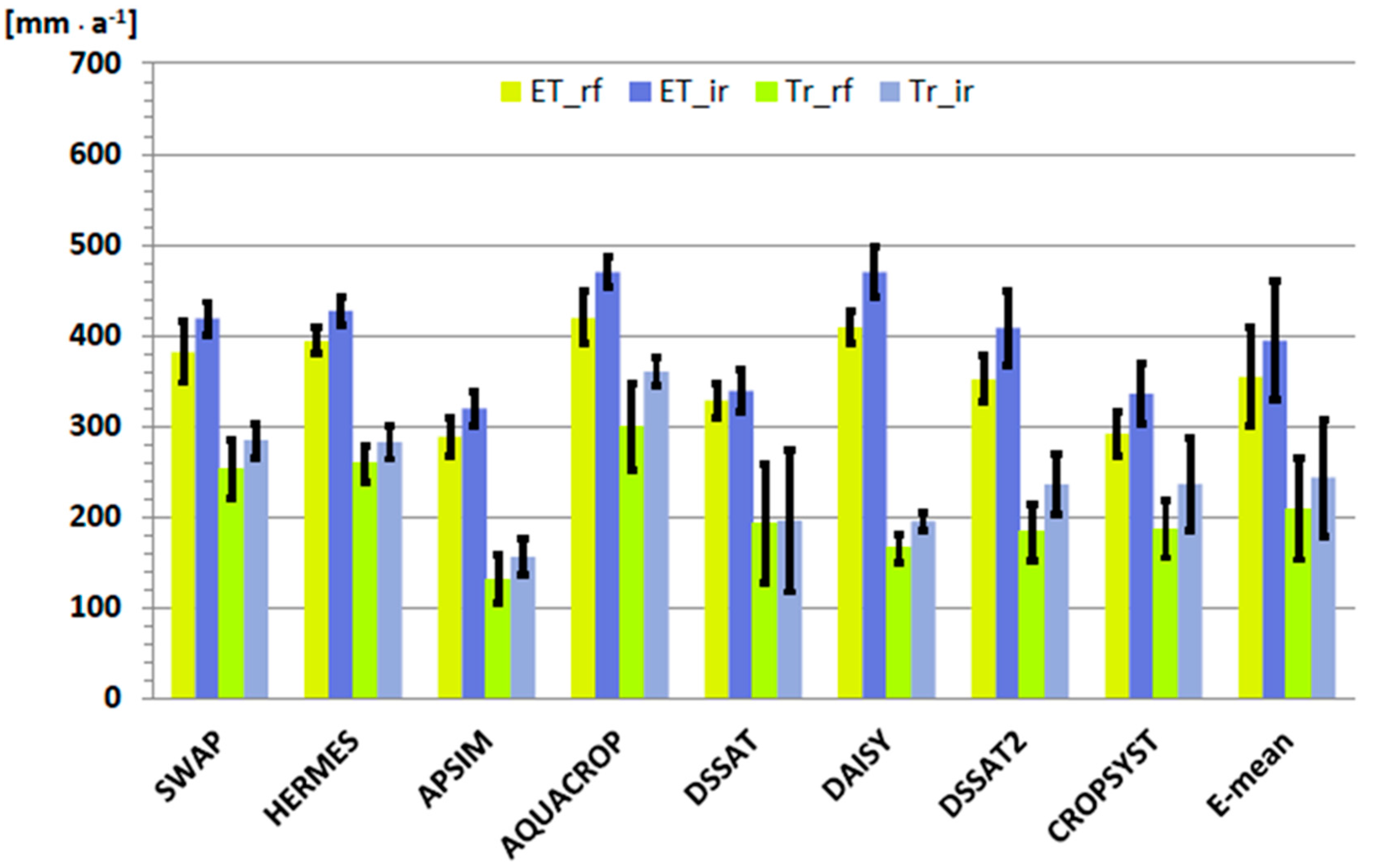
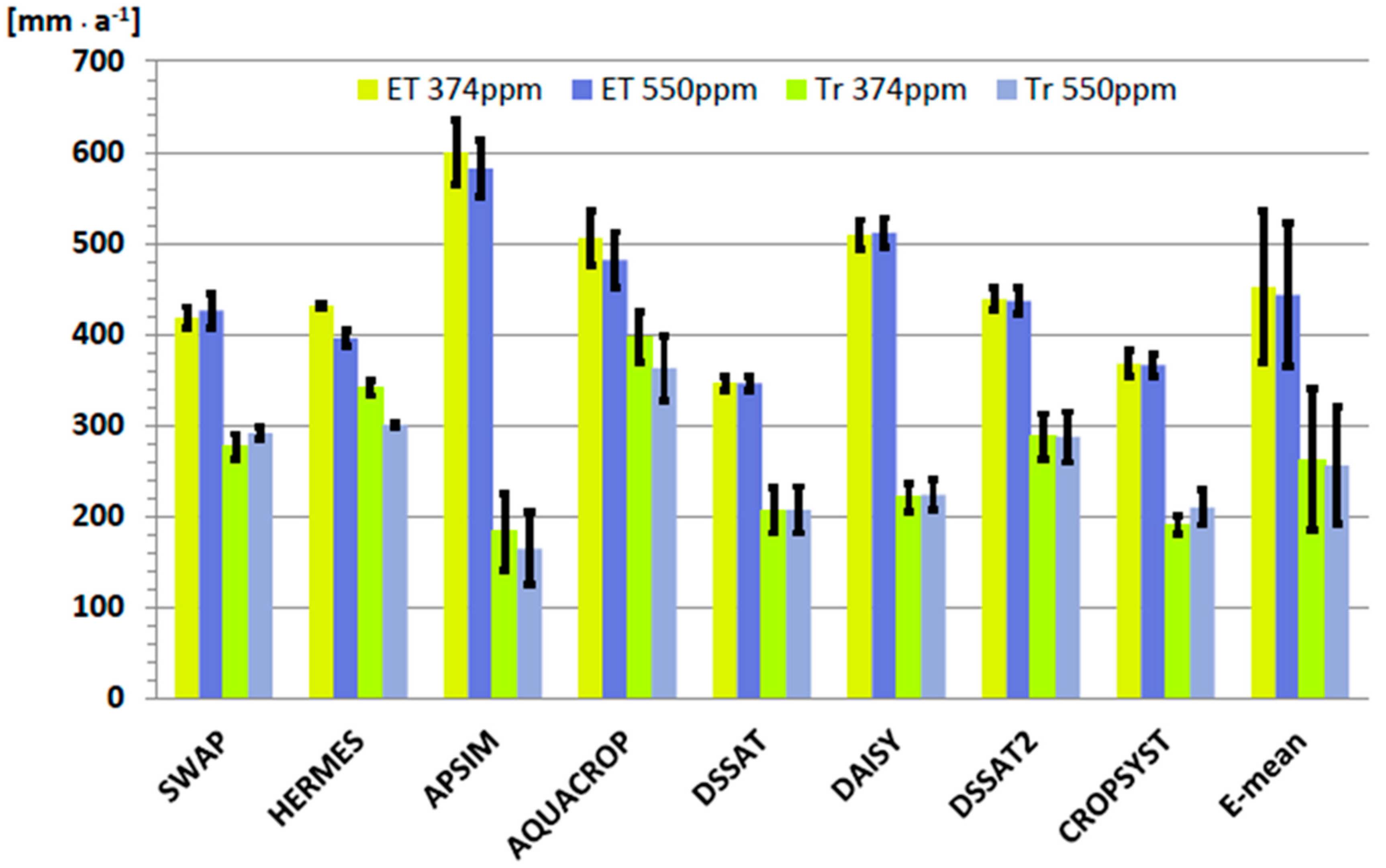
3.1. Simulated Water Consumption

The total actual evapotranspiration (ET) was simulated from sowing to harvest of the crop. Additionally, the models provided an output of the actual crop transpiration (Tr) only. Figure 2 shows both variables for the rainfed and the irrigated variants of the Müncheberg experimental site. Due to the shifted rotation, every column represents seven seasons of winter wheat. The error bars represent the inter-annual variability of the simulations of each model. The inter-annual variability of the simulated ET is relatively small with 6.3% and 5.8% on average across all models for the rainfed and irrigated variants, respectively. The absolute variation is similar for the transpiration resulting in higher coefficients of variation (CV%) due to lower absolute values of 14.7% and 12.8% for rainfed and irrigated variants, respectively. The error bars of the model ensemble mean (E-mean) represent the variation between models calculated on base of their multi-year averages. It revealed that the inter-model variability was higher than the inter-annual variability with 14.3% and 15.1% for ET and 26.8% and 26.6% for Tr of rainfed and irrigated variants, respectively. Transpiration contributes to 58% and 61% on average to the total evapotranspiration for rainfed and irrigated treatments, with the highest percentage for AQUACROP (71% and 77%) and the lowest for APSIM (45% and 49%), respectively. ET Model response to irrigation was similar showing an increase in ET and Tr, except DSSAT, which showed only a minor response.

Figure 3 shows the results of ET and Tr simulations for the FACE experiment at Braunschweig. We grouped the variants for the ambient (374 ppm) and the elevated (550 ppm) CO₂ concentration. The meaning of the error bars is similar to Figure 1. Although the variability included the variance due to the two nitrogen levels, the variability between the seasons was lower than 7% for ET and lower than 13% von Tr, except for APSIM which showed a higher variance for Tr (24%). Simulated Tr contributed on average to 59% to ET for both CO₂ concentrations ranging from 79% (374 ppm) to 76% (550 ppm) for HERMES and AQUACROP to 30% (374 ppm) to 28% for APSIM. The simulated response to elevated CO₂ was different between the models. While AQUACROP, HERMES and APSIM showed a decrease in transpiration for the elevated CO₂ concentration of 35, 40 and 18 mm, respectively, the two DSSAT simulations and DAISY showed nearly no response and CROPSYST and SWAP/WOFOST showed an increase by 15 and 19 mm, respectively. Inter-model variability was again higher than the inter-annual variability and CV% was 18% for ET and 29% and 25% for Tr at 374 and 550 ppm CO₂, respectively.

Results of the ET and Tr simulations of seven models for the lysimeters at Hirschstetten, Austria are listed in

Table 3. Simulated actual evapotranspiration (ET), transpiration (Tr), grain yield (86% d.m.) and resulting water footprints based on ET (WF) and transpiration (WF_Tr) for winter wheat on three soils at Hirschstetten/Austria from different models. WF_obs* indicate water footprints calculated from simulated ET and measured yields. Ave is the average value, ± indicates the range of simulated values around the mean and the standard deviation of the ensemble mean, CV% is the coefficient of variation between models in percent.

Model/Soil	ET (mm)			Tr (mm)		Yield (t·ha−1)			Yield obs. (t·ha−1)		WF (m3·t−1)			WF_Tr (m3·t−1)		WF_obs* (m3·t−1)
	Ave	±	CV%	Ave	±	Ave	±	CV%	Ave	±	Ave	±	CV%	Ave	±	Ave	±	CV%
APSIM S1	469	11		316	5	8.37	0.35		5.19	0.67	560	11		378	22	903
S2	351	6		187	28	4.94	0.41		2.54	0.34	713	48		375	25	1383
S3	462	22		309	38	8.49	0.58		4.94	0.37	545	11		363	20	936
AQUACROP S1	452	62		394	57	5.15	0.85		5.19	0.67	881	27		768	17	871
S2	413	61		324	48	3.64	0.91		2.54	0.34	1164	123		913	96	1629
S3	487	46		421	38	5.20	0.89		4.94	0.37	949	75		821	69	986
CROPSYST S1	286	50		167	54	5.04	1.95		5.19	0.67	620	140		341	24	551
S2	321	52		186	43	5.48	1.70		2.54	0.34	614	95		348	30	1264
S3	304	56		172	46	5.15	1.72		4.94	0.37	624	100		342	25	617
DAISY S1	494	54		265	20	7.77	1.66		5.19	0.67	652	70		351	49	953
S2	460	61		240	26	5.79	0.75		2.54	0.34	821	211		428	100	1813
S3	478	60		252	26	7.97	1.77		4.94	0.37	614	61		325	40	969
DSSAT S1	346	39		227	1	8.28	0.48		5.19	0.67	422	72		275	17	668
S2	351	16		234	17	8.41	0.89		2.54	0.34	424	64		280	10	1384
S3	362	52		253	11	8.77	1.40		4.94	0.37	417	125		290	34	733
HERMES S1	403	56		341	31	4.52	2.31		5.19	0.67	1122	450		974	430	778
S2	362	60		279	36	3.70	1.35		2.54	0.34	1060	227		829	206	1428
S3	401	38		338	12	4.53	1.73		4.94	0.37	999	298		861	302	813
SWAP/WOFOST S1	350	37		227	7	5.14	0.72		5.19	0.67	683	27		445	50	674
S2	352	40		230	8	5.17	0.93		2.54	0.34	689	53		454	69	1389
S3	352	37		231	5	5.21	0.79		4.94	0.37	681	44		451	63	712
Ensemble S1	400	76	19	277	78	6.33	1.72	27	5.19	0.67	706	230	33	505	262	771	147	19
S2	376	47	13	249	49	5.31	1.60	30	2.54	0.34	784	257	33	518	249	1470	187	13
S3	397	71	18	278	81	6.48	1.84	28	4.94	0.37	690	211	31	493	243	824	144	17

. Inter-annual variability for ET and Tr is in the order of magnitude of 17% on average with only minor differences between soils. However, only two years of winter wheat were available for each soil. Lowest ET and Tr values were simulated by most of the models for the sandy Phaeozem (S2) having the lowest capacity for plant available water. Only SWAP/WOFOST and DSSAT showed minor differences between soils. Inter-model variability varied between soils with CV% between 13% (S2) and 19% (S1) for ET and 20% (S2) and 29% (S3) for Tr. Contribution of Tr on ET was simulated highest by HERMES and AQUACROP (77%–87%), while lowest for DAISY and CROPSYST (52%–58%) with an average across all models and soils of 68%.

Table 4. Simulated actual evapotranspiration (ET), transpiration (Tr), grain yield (86% d.m.) and resulting water footprints based on ET (WF) and transpiration (WF_Tr) for winter wheat for four treatments at Foggia/Italy from different models. WF_obs* indicate water footprints based on simulated ET and measured yields. Ave is the average value, std indicates the standard deviation and CV% the coefficient of variation in percent (only for the ensemble mean).

Model/Treatment	ET (mm)			Tr (mm)		Yield (t·ha−1)			Yield obs. (t·ha−1)		WF (m3·t−1)			WF_Tr (m3·t−1)		WF_obs* (m3·t−1)
	Ave	std	CV%	Ave	std	Ave	std	CV%	Ave	std	Ave	std	CV%	Ave	std	Ave	std	CV%
APSIM T2	310	28		178	26	4.45	1.03		3.23	1.30	718	109		408	55	1206	824
T3	323	31		196	28	5.09	1.37		3.08	1.29	664	135		399	71	1418	1196
T4	334	35		209	31	5.65	1.81		3.04	1.24	637	165		393	85	1466	1210
T5	338	34		214	30	5.78	1.85		2.96	1.26	632	167		395	86	1615	1525
AQUACROP T2	340	14		222	17	3.32	0.18		3.23	1.30	1025	62		667	37	1324	234
T3	343	13		233	18	3.42	0.18		3.08	1.29	1005	80		682	54	1527	243
T4	366	25		247	25	3.57	0.29		3.04	1.24	1029	78		696	87	1532	231
T5	384	33		261	35	3.78	0.42		2.96	1.26	1022	100		696	106	1673	247
CROPSYST T2	346	25		96	33	2.31	0.73		3.23	1.30	1799	1180		413	37	1335	901
T3	345	23		98	33	2.35	0.74		3.08	1.29	1766	1186		412	38	1507	1295
T4	345	23		98	33	2.35	0.74		3.04	1.24	1766	1186		412	38	1497	1212
T5	345	23		98	33	2.35	0.74		2.96	1.26	1766	1186		412	38	1626	1507
DAISY T2	440	50		235	35	3.06	1.03		3.23	1.30	1546	410		827	239	1704	1223
T3	440	50		236	36	4.32	1.90		3.08	1.29	1201	513		647	293	1939	1750
T4	440	50		236	37	5.17	2.03		3.04	1.24	973	377		526	220	1926	1640
T5	440	50		236	37	6.07	2.24		2.96	1.26	824	328		444	183	2095	2033
DSSAT T2	283	30		146	61	4.10	2.20		3.23	1.30	926	554		383	67	1082	698
T3	298	28		179	43	5.44	1.66		3.08	1.29	591	175		336	48	1301	1114
T4	302	30		198	43	6.54	1.61		3.04	1.24	494	153		309	46	1313	1066
T5	306	31		211	42	7.37	1.53		2.96	1.26	442	148		292	48	1441	1337
HERMES T2	337	54		160	48	3.11	2.01		3.23	1.30	1709	1278		731	438	1293	932
T3	335	54		167	48	3.72	2.34		3.08	1.29	1391	975		649	411	1468	1340
T4	335	52		170	54	3.75	2.38		3.04	1.24	1386	973		651	406	1460	1258
T5	335	52		171	57	3.76	2.41		2.96	1.26	1384	974		651	406	1589	1561
Ensemble T2	343	53	15	173	51	3.39	0.77	23	3.23	1.30	1287	454	35	571	194	1327	209	16
T3	347	49	14	185	51	4.06	1.14	28	3.08	1.29	1103	447	40	521	154	1527	217	14
T4	354	47	13	193	54	4.50	1.55	34	3.04	1.24	1047	472	45	498	153	1543	209	14
T5	358	47	13	199	58	4.85	1.86	38	2.96	1.26	1012	492	49	482	158	1694	227	13

summarizes the results for the Italian site at Foggia cultivated with durum wheat. Differences of ET and Tr between the treatments were small for most of the models. Only AQUACROP, DSSAT and APSIM simulated different ET and TR amounts between treatments with a maximum difference in ET of 41 mm simulated by AQUACROP. Inter-annual variability of ET for the 10 years of each treatment were 6% (AQUACROP) to 16% (HERMES) and between 10% (AQUACROP) and 34% (CROPSYST) for Tr. However, the inter-model variability for the Italian site is slightly higher with a CV% of 13% (T5) to 15% (T2) for ET and 29% (T3,T4,T5) to 31% (T2) for Tr. Contribution of Tr to ET on average over all models and years was 53% and ranged from 28% (CROPSYST) to 67% (AQUACROP), indicating a higher portion of soil evaporation for this experimental site. Some models (APSIM, HERMES, and DSSAT) showed a stronger response of Tr to the increasing fertilization than for ET, which increased the percentage of Tr on ET, e.g., for DSSAT from 52% to 69% due to an earlier closure of the canopy.

The results for the fifth experimental site at Bratislava, Slovakia are shown in

Table 5. Simulated actual evapotranspiration (ET), transpiration (Tr), grain yield (86% d.m.) and resulting water footprints based on ET (WF) and transpiration (WF_Tr) for winter wheat for rainfed and irrigated combined with fertilized and unfertilized treatments at Bratislava/Slovakia from different models. WF_obs* indicate water footprints based on simulated ET and measured yields. Ave is the average value, std indicates the standard deviation and CV% the coefficient of variation in percent (only for the ensemble mean).

Model/Treatment	ET (mm)			Tr (mm)		Yield (t·ha−1)			Yield obs. (t·ha−1)		WF (m3·t−1)			WF_Tr (m3·t−1)		WF_obs* (m3·t−1)
	Ave	std	CV%	Ave	std	Ave	std	CV%	Ave	std	Ave	std	CV%	Ave	std	Ave	std	CV%
AQUACROP RF0	488	26		353	53	6.35	1.02		5.74	0.10	780	102		557	11	745	137
RFF	506	28		455	47	7.86	0.76		7.50	1.89	646	28		578	13	751	111
IR0	525	4		403	26	7.23	0.48		6.04	0.44	729	46		558	12	847	185
IRF	536	15		486	35	8.33	0.62		7.69	1.98	645	30		584	14	824	192
CROPSYST RF0	398	17		189	9	5.33	0.30		5.74	0.10	747	18		355	4	693	24
RFF	395	14		190	10	5.36	0.34		7.50	1.89	738	21		355	4	550	126
IR0	420	25		211	20	5.90	0.56		6.04	0.44	714	33		358	5	695	20
IRF	429	3		224	5	6.23	0.05		7.69	1.98	688	1		359	6	589	163
DAISY RF0	596	7		276	2	4.66	0.64		5.74	0.10	1299	208		601	90	1039	14
RFF	597	7		278	1	8.95	2.28		7.50	1.89	699	171		327	85	834	209
IR0	596	8		269	1	5.10	0.49		6.04	0.44	1179	135		532	57	991	65
IRF	597	8		271	1	9.67	1.47		7.69	1.98	627	90		285	43	817	212
DSSAT RF0	435	42		162	11	5.35	1.30		5.74	0.10	870	167		326	71	757	66
RFF	437	35		173	1	5.53	1.01		7.50	1.89	688	52		272	1	603	112
IR0	437	44		162	12	6.35	0.02		6.04	0.44	771	30		288	19	723	41
IRF	438	35		173	0	6.35	0.02		7.69	1.98	689	53		273	1	592	116
HERMES RF0	460	37		340	25	8.28	1.96		5.74	0.10	572	94		423	71	802	73
RFF	458	37		350	26	9.91	2.18		7.50	1.89	473	66		362	53	651	219
IR0	476	33		357	20	8.89	1.27		6.04	0.44	540	48		405	39	793	109
IRF	478	30		371	18	11.22	0.76		7.69	1.98	426	17		331	12	663	218
Ensemble RF0	475	75	16	264	86	5.96	1.43	24	5.74	0.10	854	272	32	452	122	807	135	17
RFF	479	77	16	289	117	7.69	1.85	24	7.50	1.89	649	104	16	379	117	678	114	17
IR0	491	72	15	281	100	6.56	1.52	23	6.04	0.44	786	236	30	428	115	810	117	14
IRF	495	71	14	305	125	8.36	2.15	26	7.69	1.98	615	109	18	366	127	697	117	17

for the aggregated treatments. Differences of ET between the irrigated and rainfed treatments varied between models. While DAISY and DSSAT simulated nearly no effect of irrigation, HERMES, CROPSSYST and AQUACROP showed differences of 20 to 37 mm. Interestingly, DAISY simulated even slightly lower Tr for irrigated than for rainfed treatments, which was an effect of sufficient simulated water supply under rainfed conditions on one side and of the reduction of atmospheric water demand on the irrigation days due to evaporation of water intercepted by leafs on the other hand, which led to slight reduction of transpiration for the irrigated treatments. The inter-annual variability of ET and Tr (CV%) ranged from 0.7% and 0.4% for AQUACROP and DAISY to 10% and 7.5% for DSSAT and HERMES, respectively. The inter-model variability for ET expressed as the CV% of the model ensemble was in the range of 14% to 16% (27%–34% for Tr) depending on the treatment showing a slight tendency to higher variability for the rainfed treatments. The percentage of Tr of the total ET was across all treatments and models at 58% with a maximum of 91% (IRF) and a minimum of 37% (RF0 and IR0) simulated by AQUACROP and DSSAT, respectively.

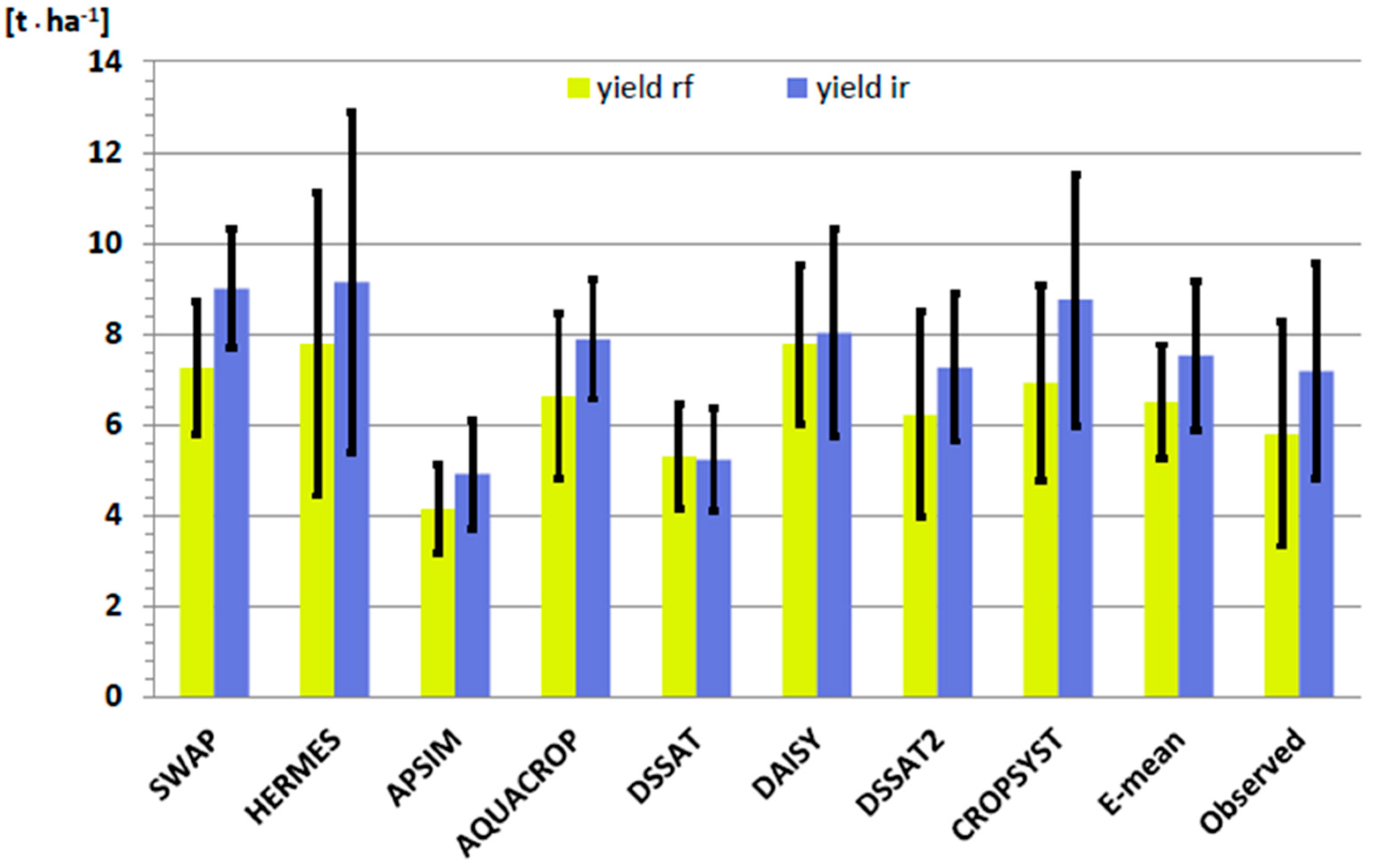
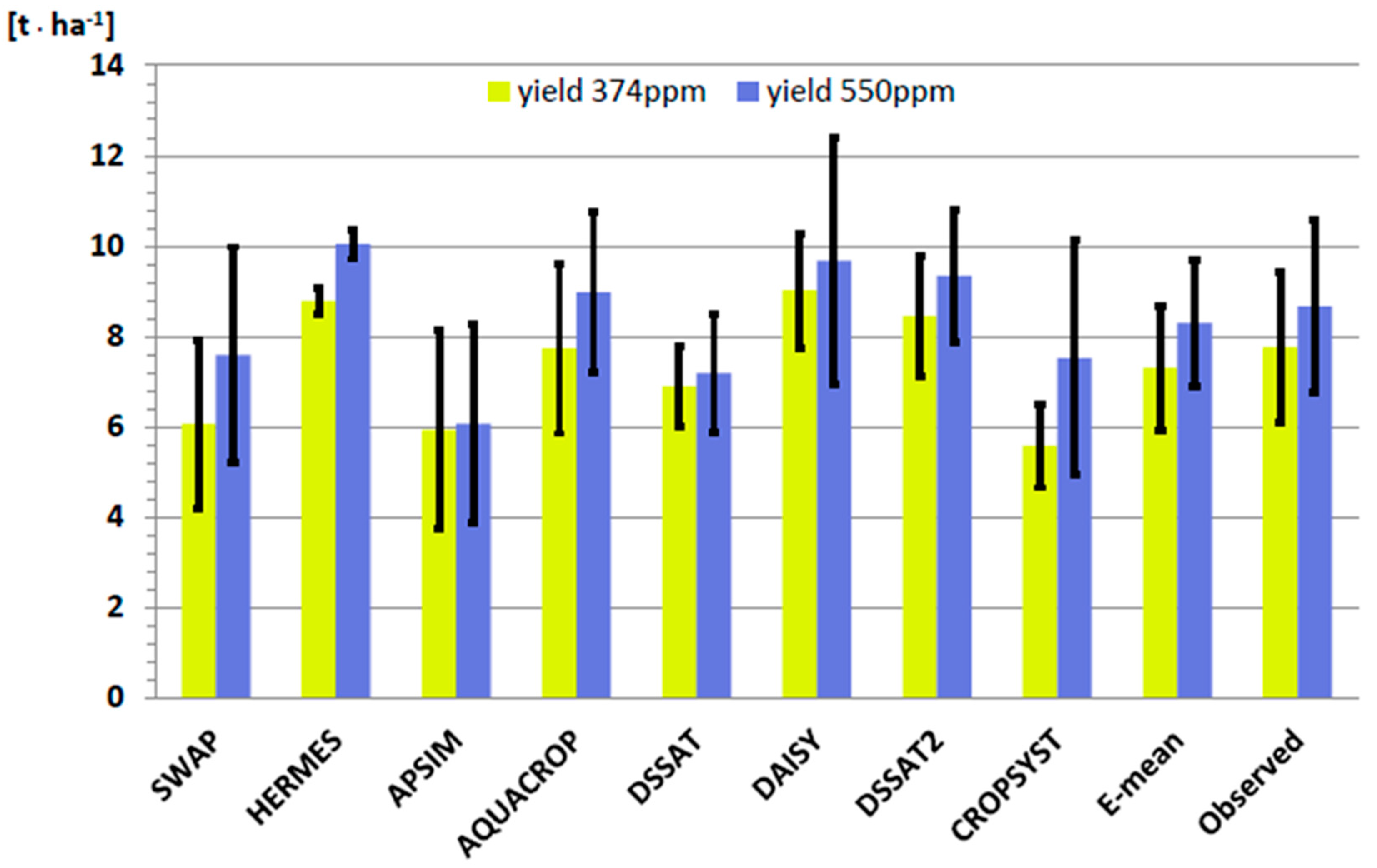
3.2. Simulated Crop Yield

For comparability, simulated and measured dry matter grain yields for winter wheat were transformed to standard yields as used in statistics by assuming a moisture content of 14%. Figure 4 shows the inter-comparison of yield estimations from eight models applied for the Müncheberg experimental site. The inter-annual variability of the yield estimations was 28% and 25% on average across all models for the rainfed and irrigated treatment, respectively. This was lower than the observed CV% of 43% and 33%, but confirmed that irrigation reduced the inter-annual variability. The ensemble mean slightly overestimated the observed grain yield by 0.7 and 0.35 t·ha⁻¹, which correspond to 12% and 5% of the observed yields. Only AQUACROP and DSSAT2 showed a similar good performance, while SWAP and HERMES overestimated and APSIM and DSSAT underestimated grain yields. The difference between the two DSAAT simulations is an indicator concerning the magnitude of user impact on model performance.

The simulated yields of the FACE experiments at Braunschweig are shown in Figure 5. As expected, all models simulated an increase of grain yields under the elevated CO₂ concentration. However, the magnitude was different ranging from 2.1% (APSIM) to 35% for CROPSYST. The ensemble mean showed a CO₂ effect of +13.6%, which was close to the observed yield increase of 11.5% as described in [32]. AQUACROP and the ensemble mean were closest to the observed yields.

Yield simulations for the more loamy soils (S1 and S3) at Hirschstetten (Table 3) showed a close fit (<0.7 t·ha⁻¹) for four out of seven models. DSSAT, APSIM and DAISY overestimated yield for these soils significantly. All models overestimated grain yield on the more sandy soil S2, which is also reflected by the ensemble mean. The inter-model variability expressed by the coefficient of variation of the ensemble mean was at 27% to 30%, which reflects a much higher model uncertainty for the yield estimation than for ET simulations.

Durum wheat yield simulations at Foggia showed even higher variations between the models (Table 4) from 25% to 39% especially for the treatments with higher fertilization. This is mainly because DAISY and DSSAT showed a strong response to the higher fertilization, while APSIM and HERMES showed no or only a slight response, which corresponds better to the observed yields showing nearly no response of crop yields as well. The simulated inter-annual variability was on average 39% ranging from 29% (APSIM) to 64% (HERMES) compared to 41% for the observed yields.

Crop yields at Bratislava (Table 5) were best estimated by the ensemble mean followed by AQUACROP. DAISY underestimated the fertilized treatments while overestimated the irrigated treatments. HERMES overestimated all treatments. The inter-model variability was 23%–26%, compared to an inter-annual CV% of 15% on average for the simulations of the rainfed treatments and 8.5% for the irrigated plots. Fertilization reduced in both cases the inter-annual variability. Inter-annual variability of observations showed CV% of 13.4% for rainfed and 16.6% for irrigated treatments. However, no fertilization reduced the observed inter-annual yield variability more than irrigation showing the lowest CV% of 1.7% and 7.3% for the rainfed and irrigated plots, respectively.

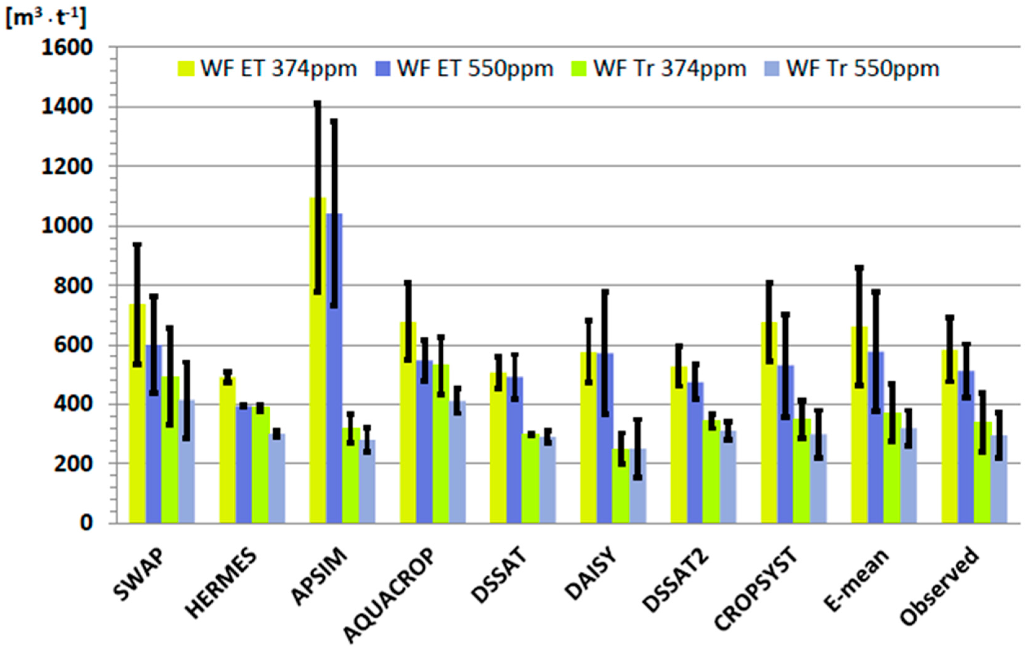
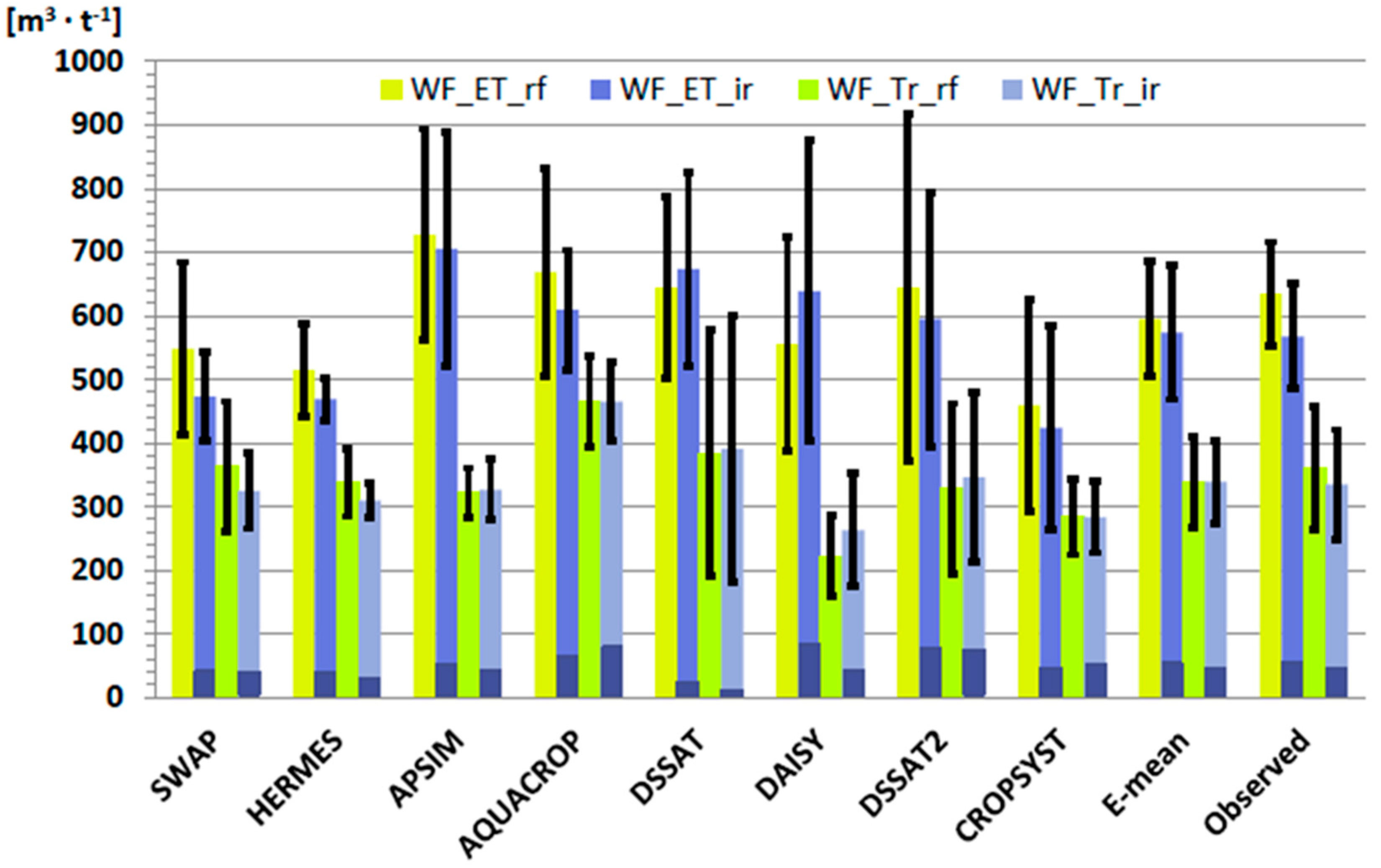
3.3. Water Footprint

Model results in Section 3.1 showed that there is a distinct difference between ET and Tr indicating that water consumption might be overestimated using ET. Therefore, we calculated water footprints alternatively using the simulated transpiration. To quantify the uncertainty caused by the inter-model variability of yield prediction we calculated the water footprint based on the simulated ET and the observed grain yields, which is annotated in Figure 6 and Figure 7 as “observed” and as “WF_obs*” in the tables. We used an overall water footprint instead of dividing it into WF_green and WF_blue for a better comparison of ranges of the model ensemble between locations.

Figure 6 contains the water footprints calculated for the Müncheberg field trial based on ET and Tr. Water footprints of the irrigated treatment were smaller than for rainfed variants for most of the models, which means that water use efficiency was higher due to a strong positive response of wheat yields on irrigation. However, DSSAT and DAISY showed an opposite trend indicating that the increase of water consumption was higher than the positive effect on crop yields. While the behavior is similar for ET and Tr based calculations for most models, the results of DSSAT2 showed an increase of WF_ET but a decrease of WF_Tr for the irrigated treatment. The inter-annual variability was estimated to be 27% on average for rainfed and 25% for irrigated treatments, which corresponded to the high inter-annual yield variability on the sandy soil (see Section 3.2). However, the variation between models for the ET based water footprint was relatively small with CV% of 15% and 18% of the rainfed and irrigated plots, respectively. Variation was slightly higher (21% for rainfed and 19% for irrigated) for the WF_Tr. Related to the estimated low contribution of Tr to the total ET, the water footprints based on Tr were on average across all models distinctly lower making 58% and 60% of the WF_ET for rainfed and irrigated treatments, respectively. Differentiation between green and blue water footprints revealed that the relative blue partition increased if Tr was used instead of ET for the calculation. The mean of the model ensemble was closer to the mean based on observed crop yields than any of the single models. DSSAT2 and AQUACROP simulations were closest on average over the two treatments.

The calculated water footprints for the two different CO₂ concentrations of the FACE experiment at Braunschweig/Germany are shown in Figure 7. All models showed a reduction of the water footprints for the elevated CO₂ concentration indicating a higher water use efficiency under higher CO₂ concentration. However, the response of DAISY and DSSAT was very low. Although SWAP showed an increase of ET and Tr (see Figure 3 in Section 3.1) with rising CO₂, this is over-compensated by the increase of yields resulting in a distinct reduction of the water footprint. Highest water footprints were calculated by APSIM, while HERMES resulted in lower values. The inter-model variability for WF_ET increases from 30% to 34% from ambient to elevated CO₂, while the CV% of WF_Tr decreased from 26% to 19%. Inter-annual variability of WF_ET was at 17% and 21% (15% and 18% for WF_Tr) on average of all models for 374 and 550 ppm, respectively.

For Hirschstetten water footprints differed among soils (Table 3). However, the effect of soil on WF_Et and WF_Tr was small for CROPSYST, DSSAT and SWAP, which corresponded to their low sensitivity of crop yields on soils (see Section 3.1). Most of the other models showed higher water footprints for the sandy Phaeozem (S2), which reflect also the trend of the water footprints calculated on the base of observed crop yields. Only HERMES simulated even higher water footprints for S1, which is mainly due to a clear underestimation of yield in the first year. The inter-model variability was 31% to 33% for the WF_ET and 48% to 52% for WF_Tr. Since the models over-predicted yields on average, the WF_ETs were under-estimated compared to the values calculated with the measured yields, which is more pronounced on the sandy soil (S2), where WF_ET was only 53% of WF_obs*.

Water footprints calculated with observed durum wheat yields showed on average over all models a slight increase with increasing nitrogen fertilization (Table 4). However, the ensemble mean of the models for WF_ET and WF_Tr showed an opposite trend. Additionally, the inter-model variability was very high and varied from 36% for treatment T2 to 55% for T5. This is mainly due to the diversity of simulated crop yield response to the treatments since the variability of water footprints calculated with observed yields was only 15% to 18%. On the other hand, WF_ET showed a very high inter-annual variability of more than 70%. Due to the low percentage of Tr on ET (see Section 3.1) the difference between WF_ET and WF_Tr is especially high for the Italian site and WF_Tr was estimated on average over all treatments to be only 43% of WF_ET.

Results for Bratislava/Slovakia (Table 5) showed about 30% higher water footprints for non-fertilized compared to fertilized treatments, while the effect of irrigation was only −8% compared to rainfed. Inter-annual variability was reduced on average from 12% to 7% from rainfed to irrigated treatments. The inter-model variability was 18% and 18% for the fertilized treatments of rainfed and irrigated plots, compared to 32% and 30% for the unfertilized plots respectively. Using the observed crop yields for the estimation of the water footprints results the variability of the unfertilized treatments distinctly, which indicates that the uncertainty originated to a large extent from uncertainty of nutrient supply from the soils.

4. Discussion

The results from five sites across Europe showed that the uncertainty in the estimation of evapotranspiration (ET) expressed through the coefficient of variation of the model ensemble was in the order of magnitude of 13% to 19%. Similar variation (15%) was observed in a comparison of nine models applied to one of the rainfed plots of the Müncheberg data set [41]. Since the absolute standard deviations of ET and Tr were in the same order of magnitude, most of the uncertainty comes from the simulation of transpiration, which showed coefficients of variation from 13% to 34% due to the lower mean value. This result was in line with findings from [28], who compared sixteen crop models regarding their uncertainty of wheat water use covering four sites across the world. He found coefficients of variation for transpiration among models from 19.8% to 33.2% and came to the conclusion that transpiration contributed most to the uncertainty to crop water use. Uncertainty from the parameterization of soil hydraulic parameters was mainly reduced since models were provided with field capacity and wilting point values for each soil profile. The same holds for the length of the growing period since flowering and ripening dates were provided for rough calibration. Most of the modelers used the trial and error approach for calibrating the phenological development of the crops. The comparison of the results from the two DSSAT groups show, that transpiration simulations at Müncheberg were quite similar, while ET values differed more. However, at Braunschweig the differences between both groups were high for Tr and ET. Differences in the initialization of soil moisture and nitrogen of the models could be a reason for the differences in ET calculation, especially because the DSSAT simulations were re-initialized every year instead of using continuous simulation over the crop rotation and initial measured values were only provided for the first year. Although this could be accounted as input error it could also be related to the model structure which makes it difficult to run the model in a continuous mode. Finally, parameter errors are related to some extent related to model structure increasing with model complexity [42]. One example might be the discussion on the Tr response to elevated CO₂ below. Beside the errors from inputs, parameters and model structure, the users of the models are another source of uncertainty [43], especially when trial and error approaches are used.

Another conclusion of the study of [28] was, that uncertainty increases with higher CO₂ concentration. However, our results from the Braunschweig FACE experiment revealed, that the coefficient of variation for the simulated transpiration at elevated CO₂ was slightly smaller than for the ambient concentration. Although some models did not reflect the reduction of water use caused by rising CO₂ concentration as it was shown in a field chamber study with wheat by [44], the beneficial effect on crop yields was reflected by all models leading to a decrease of water footprint under elevated CO₂. This was in agreement with the observed increase of water use efficiency [44]. However, the fact that reduction of water use was not reflected in some model results did not mean that the effect of increasing CO₂ on stomata resistance was not considered at all in these models. In SWAP, for example, reduction of transpiration by increased stomata resistance under elevated CO₂ was overcompensated by the increase in crop biomass and consequently in LAI. Other models use fixed or phenology driven kc factors and modify transpiration by factors (DSSAT) or by modifying stomatal resistance without considering changes in LAI (HERMES). The increase of water use efficiency or reduction in water footprints was even found under conditions of projected climate change, where potential evaporation increased due to warming [20,45].

In our study we found an increase of the estimated water footprints from North to South, which was also found in regional estimations e.g., by [15] or global studies [9,46]. Additionally, results from Bratislava showed the effect of insufficient fertilization on the water footprint, a situation, which can be often found in regions of high poverty, e.g., sub-Saharan Africa, leading to very low water use efficiency or high water footprints due to nutrient limited crop growth.

Water footprints estimated from simulated crop yields showed a high uncertainty indicated by the coefficient of variation of the model ensemble ranging from 15% to 18% for Müncheberg to 23% to 55% for the durum wheat in Foggia. Replacing simulated by observed crop yields could reduce the CV% for Hirschstetten, Foggia and Bratislava substantially leading to the conclusion that uncertainty of crop modeling contributed significantly to the uncertainty of the water footprint derived from simulated yields. Uncertainty of models was recently reported by several model inter-comparisons [23,25,27] showing very high ranges of model results for wheat yields, when models were applied only with minimum calibration. However, the inter-model variability could be significantly reduced when models are fully calibrated with suitable data for each location resulting that more than 50% of the simulated yields were below a CV% of 13.5%, which corresponds to the experimental error [25]. Uncertainty for durum wheat was higher in our study since not all models were applied for durum wheat before. In their model, inter-comparison of crop models applied for crop rotations [47] pointed out that model performance to predict crop yields was lower for crops that were not often simulated by the modelers before.

Our results for the fertilized and unfertilized plots of the Bratislava field experiment showed that nutrient limitation led to much higher inter-model variation of water footprints. Using measured crop yields reduced the CV% by 53% (from 30% to 14%). The variation in the nitrogen response of the models can add to the uncertainty of crop modeling. In their comparison of eleven models regarding their response to different nitrogen levels [48], came to the conclusion that uncertainty regarding the simulation of nitrogen release by mineralization was one of the main factors influencing the performance of crop models. Uncertainties are related to different structures of the N turnover modules in models [49], differences in their temperature responses [50] or in the estimation of initial mineralization parameters, which might be even a consequence of lacking long term history data on land management.

Soil information can have a strong influence on the regional assessment of climate impacts on crop yields [20] and water footprints [45]. The impact of soil was obvious for the lysimeters at Hirschstetten. Especially the overestimation of wheat yield for the sandy soil by some models led to a high inter-model variability and a distinctive underestimation of the water footprint compared to the calculation based on the observed yields. The uncertainty of rooting depth was identified as one major impact to the high variability and overestimation of another model ensemble for this soil [47].

Our results also indicated that the approach described in the water footprint manual [10] to use evapotranspiration for crop water use to calculate the water footprint of a crop might be worth to be discussed. We found that crop transpiration makes only 51%–68% of the total actual evapotranspiration on average across models showing a large variance between models. Similar relations were found by [28], who documented Tr to ET contributions of 56% to 77%. The rationale of the indicator is to represent consumptive water use by agricultural production at all and should be sensitive to agricultural management. However, water saving practices like advanced irrigation techniques or deficit irrigation are often applied when the crop canopy is mainly closed and soil evaporation plays a negligible role. Therefore, transpiration would be in most cases more responsive than ET, which is also shown in Figure 6 for the irrigated treatments. On average the contribution of the blue partition is 5% higher for TR compared to ET based WF. At Foggia, Tr showed a stronger response to increasing nitrogen supply compared to ET (see Section 3.1, Table 4). Other practices like mulching or tillage are mainly influencing evaporation during the time when no crop is on the soil. Therefore, these effects would not be accounted sufficiently for because the water footprint calculation just uses the ET between sowing and harvest. Inclusion of unproductive soil evaporation, which might not be accounted for the water consumption of a crop since it would occur even without crop cover, should therefore be discussed. An alternative would be to look at cropping systems as a whole including the fallow periods, but this would make it difficult to attribute the water consumption to a specific crop or product. Post-seasonal ET was not provided by all models and periods between harvest and sowing of the next crop varied due to different crop rotations, which made it difficult to compare results. For the durum wheat monoculture at Foggia, results of two models showed that post-seasonal ET contributes on average to 38% to the annual ET.

Finally, it should be noted that the model results should not be used to judge the suitability of a particular model, since information provided were basic and model performance could be certainly improved if more information would be available. We therefore did not apply model performance indicators. However, from the comparison of fully model derived water footprints to footprints using only simulated ET and observed crop yields we have to state that no model performed best on all sites and treatments and that, similar to other model inter-comparisons [19,20,21,22,23], the ensemble means were in most cases among the estimates closest to the footprints with observed yields.

5. Conclusions

The use of agro-ecosystem models is indispensable to assess impacts of climate change on crop production and resource use efficiency. However, limited opportunities to calibrate models on a regional scale and scarcity of management data at this scale imply higher uncertainties, especially regarding the prediction of crop production. Our study revealed that the uncertainty of crop yield prediction caused by the use of different models contributes more to the uncertainty in the assessment of future development of water use efficiency and water footprint calculation than the estimation of evapotranspiration. This is mainly because calculation of ET was much more standardized across the models and formulas for ET are similar. The insight that a regional calibration of crop models is recommendable to reduce uncertainty from yield predictions seems to be trivial. However, the uncertainty remains since the possibility to calibrate crop parameters for the future is limited. Recent model inter-comparisons have shown that the amount of information used for calibration has only a minor effect on most models’ climate response [51] and that crop response to external drivers, e.g., CO₂ concentration or heat stress, is still an issue of research and source of uncertainty [28,51,52]. Increasing model complexity may cause higher parameter uncertainties, which was shown in the different responses of transpiration on elevated CO₂ at Braunschweig. The choice of the most suitable model seems to be difficult since recent model inter-comparisons showed that there was no ultimate best model, which outperforms the ensemble mean or median [23,24,25,26,27].

Regarding the definition of water use for the water footprint calculation, our results indicate that the contribution of soil evaporation is not negligible and actual crop water use by transpiration is much less than the total evapotranspiration. Our results also show some evidence that Tr responds more sensitive than ET on different treatments. Therefore, the appropriateness to attribute actual seasonal evapotranspiration to crop water use requires a critical review for further water footprint and virtual water trade assessments.

References

1. Hoekstra, A.Y. Virtual Water Trade: Proceedings of the International Expert Meeting on Virtual Water Trade; Value of Water Research Report Series No 12; UNESCO-IHE: Delft, The Netherlands, 2003. [Google Scholar]
2. Hoekstra, A.Y.; Chapagain, A.K. Globalization of Water: Sharing the Planet’s Freshwater Resources; Blackwell Publishing: Oxford, UK, 2008; p. 220. [Google Scholar]
3. Allan, J.A. Virtual water: A strategic resource. Global solutions to regional deficits. Ground Water 1998, 36, 545–546. [Google Scholar] [CrossRef]
4. Hoekstra, A.Y.; Hung, P.Q. Globalisation of water resources: International virtual water flows in relation to crop trade. Glob. Environ. Chang. 2005, 15, 45–56. [Google Scholar] [CrossRef]
5. Berger, M.; Finkbeiner, M. Methodological Challenges in Volumetric and Impact-Oriented Water Footprints. J. Ind. Ecol. 2013, 17, 79–89. [Google Scholar] [CrossRef]
6. Hoekstra, A.Y.; Chapagain, A.K. Water footprints of nations: Water use by people as a function of their consumption pattern. Water Resour. Manag. 2007, 21, 35–48. [Google Scholar] [CrossRef]
7. Liu, J.; Zehnder, A.J.B.; Yang, H. Global consumptive water use for crop production: The importance of green water and virtual water. Water Resour. Res. 2009, 45, W05428. [Google Scholar] [CrossRef]
8. Mekonnen, M.M.; Hoekstra, A.Y. A global and high-resolution assessment of the green, blue and grey water footprint of wheat. Hydrol. Earth Syst. Sci. 2010, 14, 1259–1276. [Google Scholar] [CrossRef] [Green Version]
9. Siebert, S.; Döll, P. Quantifying blue and green virtual water contents in global crop production as well as potential production losses without irrigation. J. Hydrol. 2010, 384, 198–207. [Google Scholar] [CrossRef]
10. Hoekstra, A.Y.; Chapagain, A.K.; Aldaya, M.M.; Mekonnen, M.M. The Water Footprint Manual: Setting the Global Standard; Water Footprint Network Earthscan: London, UK, 2011; p. 203. [Google Scholar]
11. Jensen, M.E.; Burman, R.D.; Allen, R.G. Evapotranspiration and Irrigation Water Requirements. In ASCE Manuals and Reports on Engineering Practice; American Society of Civil Engineers: New York, NY, USA, 1990; Volume 70, p. 360. [Google Scholar]
12. Weiß, M.; Menzel, L. A global comparison of four potential evapotranspiration equations and their relevance to stream flow modelling in semi-arid environments. Adv. Geosci. 2008, 18, 15–23. [Google Scholar] [CrossRef]
13. Allen, R.G.; Pereira, L.S.; Raes, D.; Smith, M. Crop Evapotranspiration: Guidelines for Computing Crop Water Requirements; FAO Irrigation and Drainage Paper 56; Food and Agriculture Organization: Rome, Italy, 1998. [Google Scholar]
14. Smith, M.; Allen, R.; Pereira, L. Revised FAO Methodology for Crop Water Requirements. In Proceedings of the Consultants Meeting on Management of Nutrients and Water in Rainfed Arid and Semi-Arid Areas, Vienna, Austria, 26–29 May 1997; International Atomic Energy Agency: Vienna, Austria, 1998; pp. 51–58. [Google Scholar]
15. Mekonnen, M.M.; Hoekstra, A.Y. The green, blue and grey water footprint of crops and derived crop products. Hydrol. Earth Syst. Sci. 2011, 15, 1577–1600. [Google Scholar] [CrossRef] [Green Version]
16. Trnka, M.; Eitzinger, J.; Dubrovsky, M.; Semerádová, D.; Stepánek, P.; Hlavinka, P.; Balek, J.; Skala, K.P.; Farda, A.; Formayer, H.; et al. Is rainfed crop production in central Europe at risk? Using a regional climate model to produce high resolution agroclimatic information for decision makers. J. Agric. Sci. 2010, 148, 639–656. [Google Scholar] [CrossRef]
17. Trnka, M.; Olesen, J.E.; Kersebaum, K.C.; Skjelvag, A.O.; Eitzinger, J.; Seguin, B.; Peltonen-Sainio, P.; Rötter, R.; Iglesias, A.; Orlandini, S.; et al. Agroclimatic conditions in Europe under climate change. Glob. Chang. Biol. 2011, 17, 2298–2318. [Google Scholar] [CrossRef] [Green Version]
18. Wassenaar, T.; Lagacherie, P.; Legros, J.-P.; Rounsevell, M.D.A. Modelling wheat yield responses to soil and climate variability at the regional scale. Clim. Res. 1999, 11, 209–220. [Google Scholar] [CrossRef]
19. Kersebaum, K.C.; Lorenz, K.; Reuter, H.I.; Schwarz, J.; Wegehenkel, M.; Wendroth, O. Operational use of agro-meteorological data and GIS to derive site specific nitrogen fertilizer recommendations based on the simulation of soil and crop growth processes. Phys. Chem. Earth 2005, 30, 59–67. [Google Scholar] [CrossRef]
20. Kersebaum, K.C.; Nendel, C. Site-specific impacts of climate change on wheat production across regions of Germany using different CO2 response functions. Eur. J. Agron. 2014, 52, 22–32. [Google Scholar] [CrossRef]
21. Walker, W.E.; Harremoës, P.; Rotmans, J.; Van der Sluijs, J.P.; Van Asselt, M.B.A.; Janssen, P.; Von Krauss, M.P.K. Defining uncertainty: A conceptual basis for uncertainty management in model-based decision support. Integr. Assess. 2003, 4, 5–17. [Google Scholar] [CrossRef]
22. Scherer, L.; Pfister, S. Dealing with uncertainty in water scarcity footprints. Environ. Res. Lett. 2016, 11, 054008. [Google Scholar] [CrossRef]
23. Palosuo, T.; Kersebaum, K.C.; Angulo, C.; Hlavinka, P.; Moriondo, M.; Olesen, J.; Patil, R.; Ruget, F.; Rumbaur, C.; Takac, J.; et al. Simulation of winter wheat yield and its variability in different climates of Europe: A comparison of eight crop growth models. Eur. J. Agron. 2011, 35, 103–114. [Google Scholar] [CrossRef]
24. Rötter, R.P.; Palosuo, T.; Kersebaum, K.C.; Angulo, C.; Bindi, M.; Ewert, F.; Ferrise, R.; Hlavinka, P.; Moriondo, M.; Nendel, C.; et al. Simulation of spring barley yield in different climatic zones of Northern and Central Europe: A comparison of nine crop models. Field Crops Res. 2012, 133, 23–36. [Google Scholar] [CrossRef]
25. Asseng, S.; Ewert, F.; Rosenzweig, C.; Jones, J.W.; Hatfield, J.L.; Ruane, A.; Boote, K.J.; Thorburn, P.; Rötter, R.P.; Cammarano, D.; et al. Quantifying uncertainties in simulating wheat yields under climate change. Nat. Clim. Chang. 2013, 3, 827–832. [Google Scholar] [CrossRef]
26. Bassu, S.; Brisson, N.; Durand, J.-L.; Boote, K.J.; Lizaso, J.; Jones, J.W.; Rosenzweig, C.; Ruane, A.C.; Adam, M.; Baron, C.; et al. How do various maize crop models vary in their responses to climate change factors? Glob. Chang. Biol. 2014, 20, 2301–2320. [Google Scholar] [CrossRef] [PubMed]
27. Martre, P.; Wallach, D.; Asseng, S.; Ewert, F.; Rosenzweig, C.; Jones, J.W.; Hatfield, J.L.; Ruane, A.C.; Boote, K.J.; Thorburn, P.; et al. Evaluating an ensemble of 27 crop simulation models in diverse environments: Are multi-models better than one? Glob. Chang. Biol. 2015, 21, 911–925. [Google Scholar] [CrossRef] [PubMed]
28. Cammarano, D.; Rötter, R.P.; Asseng, S.; Ewert, F.; Wallach, D.; Martre, P.; Hatfield, J.L.; Jones, J.W.; Rosenzweig, C.; Ruane, A.C.; et al. Water use of wheat: Simulated patterns and sensitivity to temperature and CO2. Field Crops Res. 2016, 198, 80–92. [Google Scholar] [CrossRef]
29. Metzger, M.J.; Bunce, R.G.H.; Jongman, R.H.G.; Mucher, C.A.; Watkins, J.W. A climatic stratification of the environment of Europe. Glob. Ecol. Biogeogr. 2005, 14, 549–563. [Google Scholar] [CrossRef]
30. Mirschel, W.; Wenkel, K.-O.; Wegehenkel, M.; Kersebaum, K.C.; Schindler, U.; Hecker, J.-M. Müncheberg field trial data set for agro-ecosystem model validation. In Modelling Water and Nutrient Dynamics in Soil Crop Systems; Kersebaum, K.C., Hecker, J.-M., Mirschel, W., Wegehenkel, M., Eds.; Springer: Dordrecht, The Netherlands, 2007; pp. 219–243. [Google Scholar]
31. Mirschel, W.; Barkusky, D.; Hufnagel, J.; Kersebaum, K.C.; Nendel, C.; Laacke, L.; Luzi, K.; Rosner, G. Coherent multi-variable field data set of an intensive cropping system for agro-ecosystem modelling from Müncheberg, Germany. Open Data J. Agric. Res. 2016. [Google Scholar] [CrossRef]
32. Weigel, H.J.; Manderscheid, R. Crop growth responses to free air CO2 enrichment and nitrogen fertilization: Rotating barley, ryegrass, sugar beet and wheat. Eur. J. Agron. 2012, 43, 97–107. [Google Scholar] [CrossRef]
33. Eitzinger, J.; Trnka, M.; Hösch, J.; Zalud, Z.; Dubrovsky, M. Comparison of CERES, WOFOST and SWAP models in simulating soil water content during growing season under different soil conditions. Ecol. Model. 2004, 171, 223–246. [Google Scholar] [CrossRef]
34. Ventrella, D.; Stellacci, A.M.; Castrignanò, A.; Charfeddine, M.; Castellini, M. Effects of crop residue management on winter durum wheat productivity in a long term experiment in Southern Italy. Eur. J. Agron. 2016, 77, 188–198. [Google Scholar] [CrossRef]
35. Steduto, P.; Hsiao, T.; Raes, D.; Fereres, E. AquaCrop-The FAO crop model to simulate yield response to water: I. Concepts and underlying principles. Agron. J. 2009, 101, 426–437. [Google Scholar] [CrossRef]
36. Keating, B.A.; Carberry, P.S.; Hammer, G.L.; Probert, M.E.; Robertson, M.J.; Holzworth, D.; Huth, N.I.; Hargreaves, J.N.G.; Meinke, H.; Hochman, Z.; et al. An overview of APSIM, a model designed for farming systems simulation. Eur. J. Agron. 2003, 18, 267–288. [Google Scholar] [CrossRef]
37. Hansen, S.; Abrahamsen, P.; Petersen, C.T.; Styczen, M. Daisy: Model use, calibration and validation. Trans. ASABE 2012, 55, 1315–1333. [Google Scholar] [CrossRef]
38. Jones, J.W.; Hoogenbohm, G.; Porter, C.H.; Boote, K.J.; Batchelor, W.D.; Hunt, L.A.; Wilkens, P.W.; Singh, U.; Gijsman, A.J.; Ritchie, J.T. The DSSAT cropping system model. Eur. J. Agron. 2003, 18, 235–265. [Google Scholar] [CrossRef]
39. Kroes, J.G.; van Dam, J.C.; Groenendijk, P.; Hendriks, R.F.A.; Jacobs, C.M.J. SWAP Version 3.2(26). Theory Description and User Manual; Alterra-Report; Alterra Research Institute: Wageningen, The Netherlands, 2009; Volume 1649, p. 284. [Google Scholar]
40. Stöckle, C.O.; Donatelli, M.; Nelson, R. CropSyst, a cropping systems simulation model. Eur. J. Agron. 2003, 18, 289–307. [Google Scholar] [CrossRef]
41. Kersebaum, K.C.; Hecker, J.M.; Mirschel, W.; Wegehenkel, M. Modelling water and nutrient dynamics in soil-crop systems: A comparison of simulation models applied on common data sets. In Modelling Water and Nutrient Dynamics in Soil-Crop Systems; Kersebaum, K.C., Hecker, J.-M., Mirschel, W., Wegehenkel, M., Eds.; Springer: Dordrecht, The Netherlands, 2007; pp. 1–17. [Google Scholar]
42. Grunwald, S. GIS Gestürtzte Modellierung des Landschaftswasser und Stoffhaushalts mit dem Modifizerten Modell AGNPSm. Ph.D. Thesis, University Giessen, Giessen, Germany, 1997. [Google Scholar]
43. Confalonieri, R.; Orlando, F.; Paleari, L.; Stella, T.; Gilardelli, C.; Movedi, E.; Pagani, V.; Cappelli, G.; Vertemara, A.; Alberti, L.; et al. Uncertainty in crop model predictions: What is the role of users? Environ. Model. Softw. 2016, 81, 165–173. [Google Scholar] [CrossRef]
44. Manderscheid, R.; Weigel, H.-J. Drought stress effects on wheat are mitigated by atmospheric CO2 enrichment. Agron. Sustain. Dev. 2007, 27, 79–87. [Google Scholar] [CrossRef]
45. Kersebaum, K.C. Effects of climate change and elevated CO2 on wheat water consumption, yield and water footprint in three contrasting regions of Germany. Ital. J. Agromet. 2015, Si, 117–122. [Google Scholar]
46. Fader, M.; Rost, S.; Müller, C.; Bondeau, A.; Gerten, D. Virtual water content of temperate cereals and maize: Present and potential future patterns. J. Hydrol. 2010, 384, 218–231. [Google Scholar] [CrossRef]
47. Kollas, C.; Kersebaum, K.C.; Nendel, C.; Manevski, K.; Müller, C.; Palosuo, T.; Armas-Herrera, C.M.; Beaudoin, N.; Bindi, M.; Charfeddine, M.; et al. Crop rotation modelling—A European model intercomparison. Eur. J. Agron. 2015, 70, 98–111. [Google Scholar] [CrossRef]
48. Salo, T.; Palosuo, T.; Kersebaum, K.C.; Nendel, C.; Angulo, C.; Ewert, F.; Bindi, M.; Calanca, P.; Klein, T.; Moriondo, M.; et al. Comparing the performance of eleven crop simulation models in predicting yield response to nitrogen fertilisation. J. Agric. Sci. 2016, 154, 1218–1240. [Google Scholar] [CrossRef]
49. Gabrielle, B.; Mary, B.; Roche, R.; Smith, P.; Gosse, G. Simulation of carbon and nitrogen dynamics in arable soils: A comparison of approaches. Eur. J. Agron. 2002, 18, 102–120. [Google Scholar] [CrossRef]
50. Rodrigo, A.; Recous, S.; Neel, C.; Mary, B. Modelling temperature and moisture effects on C-N transformations in soils: Comparison of nine models. Ecol. Mod. 1997, 102, 325–339. [Google Scholar] [CrossRef]
51. Ruane, A.C.; Hudson, N.I.; Asseng, S.; Camarrano, D.; Ewert, F.; Martre, P.; Boote, K.J.; Thorburn, P.J.; Aggarwal, P.K.; Angulo, C.; et al. Multi-wheat-model ensemble responses to interannual climate variability. Environ. Model. Softw. 2016, 81, 86–101. [Google Scholar] [CrossRef]
52. Asseng, S.; Ewert, F.; Martre, P.; Rötter, R.P.; Lobell, D.B.; Cammarano, D.; Kimball, B.A.; Ottman, M.J.; Wall, G.W.; White, J.W.; et al. Rising temperatures reduce global wheat production. Nat. Clim. Chang. 2015, 5, 143–147. [Google Scholar] [CrossRef]
Figure 1. Location of the experimental sites.
Water 08 00571 g001
Figure 2. Simulated evapotranspiration (ET) and transpiration (Tr) for rainfed (_rf) and irrigated (_ir) variants of the Müncheberg field experiment from different models. Error bars of the model results show inter-annual variability, error bars of the ensemble mean the inter-model variability.
Water 08 00571 g002
Figure 3. Simulated evapotranspiration (ET) and transpiration (Tr) for ambient (374 ppm) and elevated (550 ppm) atmospheric CO2 concentration of the Braunschweig FACE experiment from different models. Error bars of the model results show inter-annual variability, error bars of the ensemble mean the inter-model variability.
Water 08 00571 g003
Figure 4. Simulated grain yields of winter wheat for rainfed (_rf) and irrigated (_ir) variants of the Müncheberg field trial from different models. Error bars of the model results and observations show inter-annual variability, error bars of the ensemble mean the inter-model variability.
Water 08 00571 g004
Figure 5. Simulated winter wheat grain yields for ambient (374 ppm) and elevated (550 ppm) atmospheric CO2 concentration of the Braunschweig FACE experiment from different models. Error bars of the model results and observations show inter-annual variability, error bars of the ensemble mean the inter-model variability.
Water 08 00571 g005
Figure 6. Water footprints of winter wheat calculated from simulations of different models for rainfed (_rf) and irrigated (_ir) variants of the Müncheberg field trial. Calculations were based on ET (WF_ET) and Tr (WF_Tr). Error bars of the model results and observations show inter-annual variability, error bars of the ensemble mean the inter-model variability. “Observed” is calculated from simulated ET and Tr and observed yields. Dark blue columns in WF_ET_ir and Tr_ir show the blue WF based on ET and Tr, respectively.
Water 08 00571 g006
Figure 7. Water footprints of winter wheat calculated from simulations of different models for ambient (374 ppm) and elevated (550 ppm) CO2 concentrations of the FACE experiment at Braunschweig/Germany. Error bars of the model results and observations show inter-annual variability, error bars of the ensemble mean the inter-model variability. “Observed” is calculated from simulated ET and Tr and observed yields.
Water 08 00571 g007