Canals vs. Streams: To What Extent Do Water Quality and Proximity Affect Real Estate Values? A Hedonic Approach Analysis

Abstract

The presence of and proximity to water influences human settlement decisions, because water has been able to characterize the environment and affect human health since prehistoric times. Many scholars have studied the effects of environmental amenities on the real estate market; however, only a few of them have explored the effects of water. This study stresses the role of water with a focus on the dichotomy between artificial and natural waterways (canals vs. streams), which involves managerial and qualitative differences. A hedonic approach, based on a large web scraped and geo-referenced dataset of 10,530 observations, is used to analyze the effect of water proximity and quality on residential housing prices in the province of Milan (Italy). Our main results show a significant but conflicting impact of water proximity on real estate value: reducing the canal distance, we observe an increase in the residential housing sale price, in urban more than peri-urban environments; in contrast, reducing the stream distance, our results show decreases in property value. Moreover, a significant moderating effect of water quality on distance from streams is identifiable.

1. Introduction

In rural areas, i.e., outside the city, water is a critical element because it is strongly related to agricultural utilization. In contrast, in fragmented and highly urbanized areas, water is able to produce several positive amenities, such as preserving natural ecosystems [1], mitigating the impacts caused by human activity, such as air pollution and heat islands [2,3,4,5] and providing aesthetically pleasing open spaces and recreational sites [6,7,8]. However, in spite of these positive amenities, some researchers have specifically focused only on the aptitude of water to leverage the real estate market by influencing property values.

In this light, the effect of surface water bodies on residential housing prices has been specifically related to different features such as water proximity, security and quality. Walsh et al. (2011) [9] identified the significance of water body proximity on the value of residential properties in Orange County, Florida. Positive amenities from proximity to water are also reported by Anderson and West (2006) [10]. Tapsuwan et al. (2009) [11] argue that the value of houses increases by reducing the distance to the wetland. Cohen et al. (2014) [12] show conflicting findings for proximity to wetlands but confirm the positive effect of water bodies’ proximity. Cho et al. (2006) [13] suggest the influence of proximity to creeks and streams in Tennessee. Nelson et al. (2005) [14] highlight the positive effect of proximity to artificial water bodies. Other studies focus on water views rather than spatial proximity and suggest surface water is able to increase the waterfront property value [15].

Conversely, some studies suggest that some drawbacks of being located near water bodies are potentially due to the perception of flood risk [16]. Climate change, deforestation and urbanization have been constantly increasing the incidence of flooding, despite the development of water management programmes. Thus, the location within a zone where flooding probability is higher may reduce the value of property and negatively influence the transaction price [17,18]. This suggests that the wish to live near water bodies could be moderated by the need for safety. However, the perceived risk does not only depend on probability and impact of events but also on environmental vulnerability. Accordingly, the implementation of good managerial practices such as rainwater harvesting systems in urban and peri-urban environments is able to minimize the flooding risk [19] by increasing structural resilience to hydrological events.

Furthermore, several studies have also stressed the role of water quality on property value [9,20,21,22]. Water quality is a feature potentially influencing the significance of proximity. People are not inclined to pay more for proximity to waterways characterized by a bad-smelling and unpleasant ecological status. Other studies have focused on water clarity [23,24,25]. Recently, Bin et al. (2016) [26] performed a segmented regression analysis where water quality improvement is proven to be associated with higher housing prices in Florida.

In sum, analysis of the literature suggests that water proximity, quality and security have been shown to be important, mutually dependent, predictors of property value. However, despite water’s growing popularity, its impact is not clearly quantifiable and can depend on multiple research considerations such as water features, water body nature, environmental background or real estate market structure.

This study attempts to measure the influence of water proximity on the real estate market of the province of Milan in Italy by distinguishing between canals and streams. This dichotomy is introduced for different reasons. First, a number of studies can be identified distinguishing between water bodies and wetlands [12], but no comparison was found between natural and artificial waterways. Second, it allows the indirect measurement of the effect of water security because of the more effective management of flood risk in artificial rather natural water bodies. Third, water in canals is regarded as having a better ecological status because of more control and management practices being performed. Nonetheless, a measure of local surface water quality, as provided by Regional Agency for Environmental Protection of Lombardy (ARPA) in terms of ecological and chemical status, has been introduced in order to control for the interactive effect between quality and proximity.

Therefore, this study contributes to a better understanding of the role of water in the real estate market of urban and semi-urban environments, and specifically explores the differences in the proximity effect of canals vs. streams and the moderating effect of related water quality.

In this work, a hedonic approach, as proposed by Cheshire and Sheppard (2002) [27], is applied to investigate the effect of water proximity and quality on the real estate market of the province of Milan. A very large database, as compared to several studies on this topic, consisting of 10,802 observations, has been collected by integrating web scraping and geo-referenced techniques. A spatial semi-logarithmic regressive model is operationalized in order to control for the potential spatial dependence of housing prices. Firstly, structural features of properties and territory are included as controls in the base model. Then, the distance of the property from the nearest canal and stream and the value of relative water quality are specifically explored; their interaction is also included in order to control for the potential moderating effect of quality on proximity.

This study has produced some interesting results. If moving away from canals leads to a decrease in housing prices, a larger distance from streams increases the property value; however, differently from canals, the impact of proximity to streams is strongly moderated by the quality of the water. Finally, different results on the role of canals are shown concerning urban and semi-urban environments.

The next section is dedicated to describing the background context in order to highlight the water bodies’ territory features, in terms of quality and security. The third section explains the methodological approach, focusing on data collection, variables definition and regressive techniques explanation. The analysis results are discussed in the fourth section. Conclusions follow in the final section.

2. Background Context

This study focuses on the province of Milan which is one of the most populous urban environments in Europe (about 3,181,152 inhabitants distributed over an area of 1578.9 km²) and the largest Italian real estate market (also as a result of urban development and revitalization linked to the world exposition event-EXPO 2015).

The territory is located in the high stretch of the Po valley between the river Ticino to the West and the river Adda to the East and is crossed by several waterways such as streams (Olona, Lambro, Seveso), creeks (Lura, Bozzente, Molgora, Arno) and a large network of canals inside and outside Milan city (Naviglio Grande, Martesana, Pavese Canal).

The Po, which is the main Italian river for water flow, runs away in the southern valley. The second most important rivers in the area are Ticino and Adda but they constitute the boundaries of the territory and produce only marginal environmental effects. Thus, even though the province of Milan is strongly characterized by water presence, local water bodies are classified as streams or canals.

The more important canals cross the urban area of Milan, sometimes up to the central zones of the city. The streams flow marginally into the city in the peripheral neighborhoods. Outside the city, other urban centers of significant size, with developed industrial activities, can be found along the streams. The large volume of business activities necessarily affects the quality of the water bodies flowing through the Milanese area. Similarly, the large number of inhabitants makes sewage a critical issue.

In this context, the monitoring and control of the ecological and chemical status of waterways by ARPA provides some critical considerations concerning the quality of water. Data (see Figure 1) provided by detection stations in 2014 (the last available value by ARPA) [28] highlight the overall value of surface water quality in the area as being very low (2.2). However, canal water is, on average, significantly (Anova test: p-value = 0.025) better than stream water (2.66 vs. 2.00).

Another important point concerns water security and flood risk. Although the National Civil Protection classifies the Milan area as a hydro-geological risk area, the territory management and governance as well as the low size of local water bodies decrease the environmental vulnerability and the impact of flooding events in the area. Moreover, the effectiveness of water security practices is traditionally higher for canals than streams, because of structural features and the management of water flows. In conclusion, since the flood risk in the Milanese area is very low (because of low probability and limited impact), in the next sections, we mainly focus on the role of water quality and proximity as leveraging residential housing prices.

3. Methodology

The recurring primary method used systematically in the international literature for studies on environmental issues is the hedonic price model. According to the neoclassical approach, when a consumer pays a price for the purchase of a complex good, which is a good that incorporates many attributes (such as a car, a house, a computer, etc.), his/her choice is based on his/her individual utility function. Then, the price that was paid can be broken down into implicit prices of individual variables that comprise the good, which allows us to bring a single explicit piece of data (the sale price) to many other data that correspond to the value of each single variable. These concepts have been investigated by Griliches (1971) [29] and Rosen (1974) [30] who developed the model of analysis from the general equilibrium conditions that were indicated by Strotz (1968) [31].

In the literature, hedonic techniques are widely used to estimate the value of environmental amenities that do not have a market but are indirectly capitalized on in the value of residential units [23]. Applying the hedonic model to the property market allows us to highlight the implicit values of water features through the study of the sale price of the properties.

The variables used in the various studies are quite different, and vary in function by specific site situation, in order to adapt the model to the analytical context in relation to the available sources of data. From an analysis of the literature, three main categories of variable can be identified: structural, environmental and territorial variables [32]. The first set of variables consists of all the variables that characterize the structural aspects of properties. The territorial variables are used to contextualize the location and characteristics of the property in the territorial context of reference. Finally, the environmental variables allow us to summarize the characteristics of the environmental resources, in our specific case, the role of water bodies in terms of proximity and quality on house prices.

3.1. Data Description

The research study aims to explore the role of water proximity and quality as leveraging the property value in the real estate market. The study area is the whole province of Milan. The unit of analysis is the residential properties for sale.

Since in Italy no official data on house sale prices are available, a database was created by web scraping the data relating to real estate for sale in the province of Milan on 7 July 2015 from the website of a consenting real estate agency. This procedure may produce some potential weaknesses that need to be highlighted. First, the scraped prices are not sale prices but bid prices since they do not consider any real negotiation of sale. Even though the sale price is typically inclined to be lower than the bid price, the price reduction rate is casually distributed because it depends on personal issues (e.g., the time to market, the need for money) more than environmental features. Therefore, we retain bid price as a good proxy of sale price. Second, despite the data being from web scraping, the downloaded sale prices are defined in a little less than a four-year window, from 24 October 2011 to 7 July 2015. Thus, the insertion year on which the bid price has been entered is adopted as a control variable in order to assess the potential time trend. Given the impressive amount of available data, we used crawler software (in this study, we used the software Web Content Extractor 7.2^® (Mountain View, CA, USA). It is a crawler software able to simulate the human browsing experience by replicating computer commands to browse, search, navigate, and ultimately extract specific data fields from a web page) to automatically download the data and construct the database. The resulting dataset consisted of approximately 38,000 observations, including the house selling price information and the structural characteristics of each property, such as the number of rooms, number of bathrooms, surface in square meters, status of the property, type of kitchen, presence of an elevator, basement, or garage, type of garden, energy class, date of the announcement, total number of floors of the building, condition of the building (new, to be renovated, etc.), monthly condominium fees, and finally, the address of the property.

Based on this last information, each residential unit was geo-referenced by means of a software called “Google Earth Pro 7.1.5^®” (Mountain View, CA, USA). The database was reduced to approximately 27,000 data points because of a lack of address information or of errors invalidating the geo-referencing process. The coordinates make it possible to map the properties for sale on the map and to use GIS (The GIS software used is Arcgis 10.2.2^®, Redlands, CA, USA) software for computing spatial variables (the function Near in the Analysis Tools of Arcgis is used to calculate the shortest distance, i.e., “as the crow flies”, between the point relative to each individual property and the nearest point of the resource or of the territorial component being analyzed), such as distance from the city center, subway and rail stations, malls and water bodies.

Finally, due to missing values in at least one of the structural variables and the exclusion of the first and ninetieth percentile of the house price distribution to eliminate the influence of any possible outliers, we obtained our final sample of 10,530 observations (we checked that the loss of observations was distributed randomly over the entire territory and was not related to specific areas; thus, we expect the findings should not be biased). 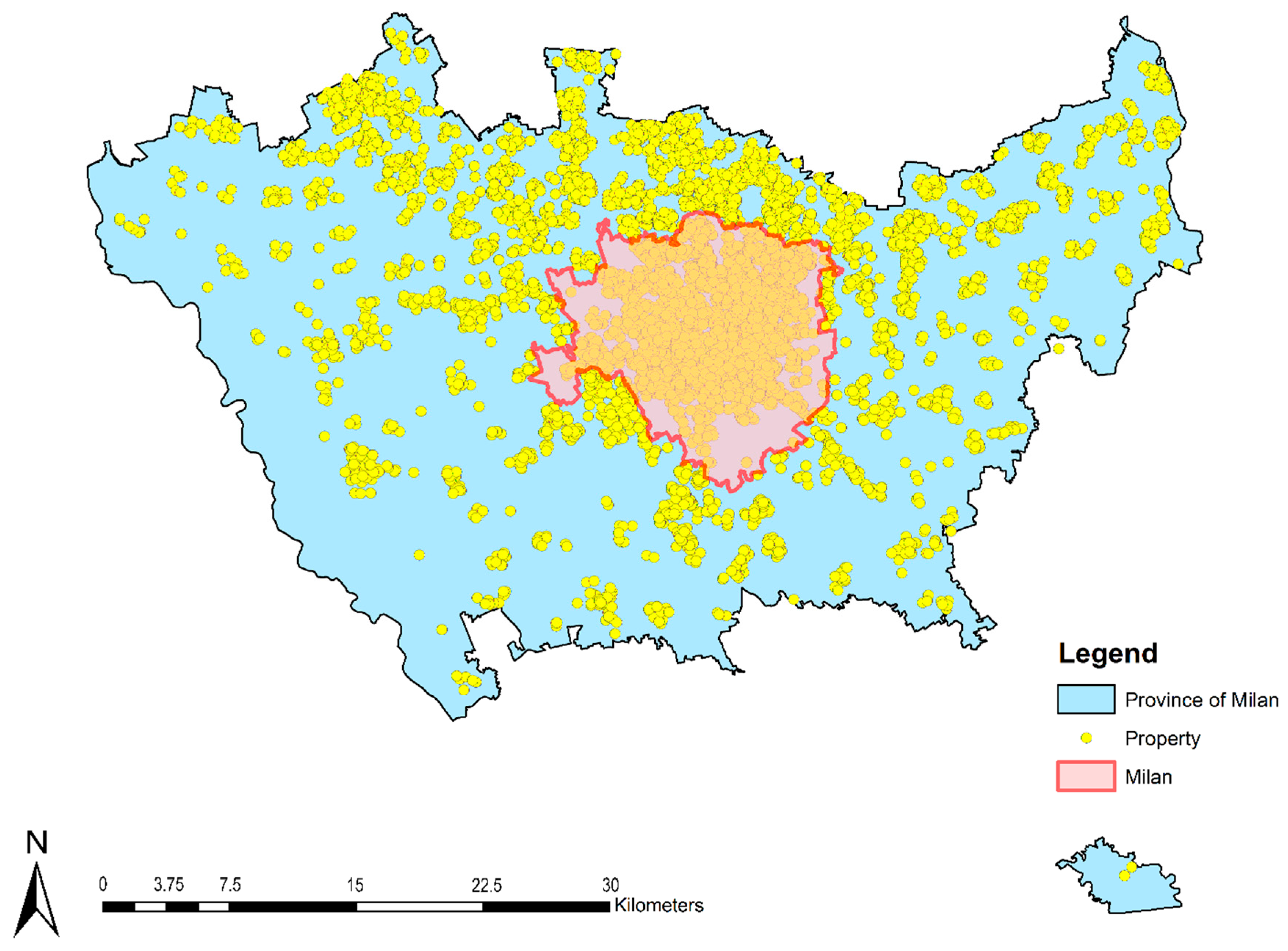Figure 2 shows the spatial distribution of the data points in the city of Milan and across the province. 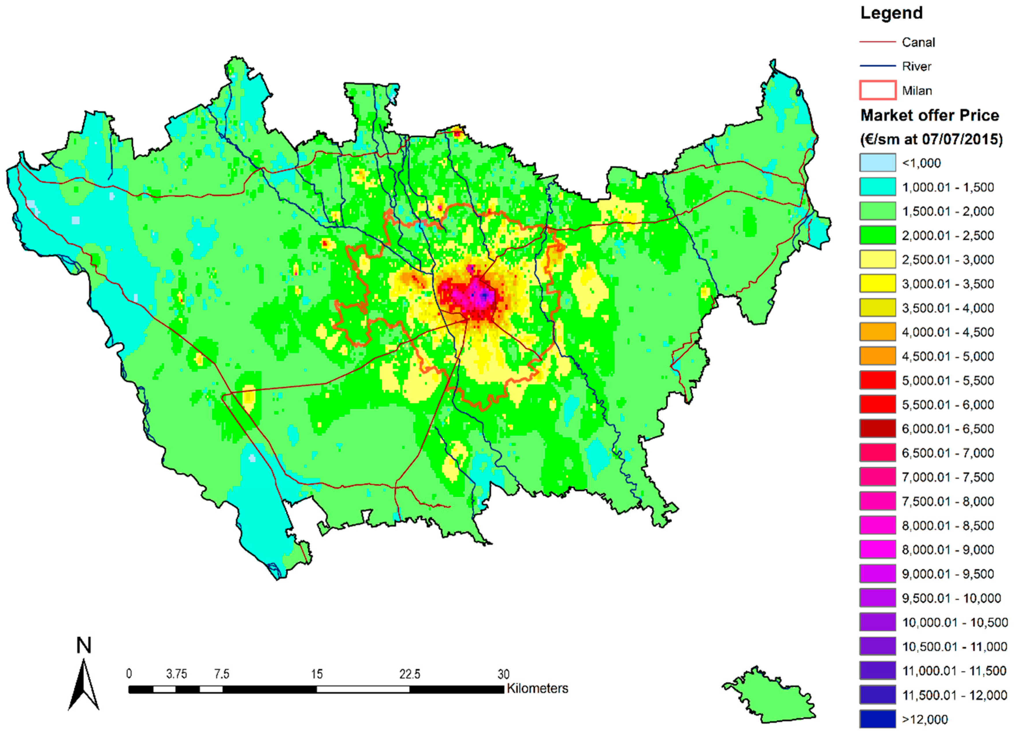Figure 3 shows the real estate market zones based on house selling prices.

3.2. Variables

3.2.1. Control Variables

Structural Variables

The intrinsic variables that were used for regression analysis include energy class (in parentheses are the names used for the analysis of the variables and a brief description) (energ_class indicates the energy class expressed in kWh/m²), the surface of the house in square meters (surf_sm), monthly condominium fees (cond_fees refers to the monthly service charges), immediate availability of the property (free_dummy for which 1 = immediately free and 0 = busy), the kitchen type (kitch_type_dummy for which 1 = habitable living space and 0 = not a habitable living space), the presence of an elevator (elevat_dummy for which 1 = present and 0 = absent), the presence of a balcony (balcony_dummy for which 1 = present and 0 = absent), the presence of a garage (garage_dummy for which 1 = present and 0 = absent), the home furnishings (furnish_type_dummy for which 1 = furnished and 0 = unfurnished) and the status of the property (prop_stat_1 = new property, prop_stat_2 = entirely renovated, prop_stat_3 = habitable, prop_stat_4 = to be renovated). We also included time control dummy variables for each year (year_dummy) for the period from 24 October 2011 to 7 July 2015 to take account of any potential time trend in our data. In

Table 1. Descriptive statistics.

Variable	Min.	Max.	Mean	St.Dev.
price	30,000.00	6,000,000.00	298,067.74	315,446.92
dist_stream	4.14	11,655.59	2242.70	2044.67
quality_stream	1.00	4.00	1.99	1.09
dist_canal	4.42	22,572.51	2180.31	1862.66
quality_canal	3.00	4.00	3.38	0.48
energ_class	2.50	949.31	167.00	80.94
sup_mq	25.00	700.00	100.34	53.24
cond_fees	10.00	15,000.00	193.24	387.28
dist_sub_st	6.08	35,681.82	3915.94	5781.94
dist_tr_st	15.02	20,054.64	2077.59	1751.21
dist_mall	17.13	23,496.05	1427.36	1160.64
green_area	0.00	142,176.90	19,384.62	21,617.61
year_dummy_2011	0	1	0.49	0.45
year_dummy_2012	0	1	0.10	0.29
year_dummy_2013	0	1	0.12	0.32
year_dummy_2014	0	1	0.21	0.40
year_dummy_2015	0	1	0.09	0.28

and

Table 2. Descriptive statistics of dichotomous variables.

Variable	Item	Absolute Frequency	Relative Frequency in %
kitch_typ	Livable	6654	63.19
	Not livable	3876	36.81
	Total	10,530	100.00
elevat	Yes	7682	72.95
	No	2848	27.05
	Total	10,530	100.00
balcony	Yes	7790	73.98
	No	2740	27.02
	Total	10,530	100.00
box	Yes	4977	47.26
	No	5553	52.74
	Total	10,530	100.00
furnish_type	Furnished	3054	29.00
	Unfurnished	7476	71.00
	Total	10,530	100.00
prop_status	prop_stat1	1092	10.37
	prop_stat2	4850	46.06
	prop_stat3	3816	36.24
	prop_stat4	772	7.33
	Total	10,530	100.00

Notes: The distribution of the 96 Milan province zip codes is not reported due to spatial constraints.

a summary of the variables employed in our analysis is reported.

The other variables were discarded during correlation analysis, which indicates highly correlated variables (see

Table 3. Correlation matrix.

Variables	1	2	3	4	5	6	7	8	9	10	11	12	13	14	15	16	17	18	19	20	21
1 price	1
2 dist_stream	−0.03 ***	1
3 quality_stream	0.06 ***	0.00	1
4 dist_canal	−0.18 ***	−0.07 ***	−0.04 ***	1
5 quality_canal	0.02 *	0.00	−0.17 ***	−0.01	1
6 energ_clas	−0.07 ***	−0.05 ***	−0.01	0.01	−0.03 **	1
7 sup_mq	0.74 ***	0.01	0.04 ***	−0.03 ***	0.02 *	−0.08 ***	1
8 cond_fees	0.42 ***	−0.03 **	0.02 *	−0.05 ***	0.02 *	0.01	0.29 ***	1
9 kitch_type	0.24 ***	0.01	0.03 **	0.03 ***	0.00	0.04 ***	0.42 ***	0.12 ***	1
10 elevat	0.13 ***	−0.09 ***	0.02 *	−0.04 ***	0.01	−0.14 ***	−0.01	0.11 ***	0.07 ***	1
11 balcony	0.04 ***	−0.02 *	−0.01	0.07 ***	0.01	0.02 *	0.12 ***	0.05 ***	0.21 ***	0.08 ***	1
12 box	0.08 ***	0.10 ***	−0.01	0.12 ***	0.02 *	−0.23 ***	0.29 ***	0.02 *	0.18 ***	0.01	0.08 ***	1
13 furnish_type	0.04 ***	−0.02 *	0.06 ***	−0.05 ***	0.01	0.04 ***	−0.05 ***	−0.01	−0.10 ***	−0.01	−0.08 ***	−0.08 ***	1
14 prop_status_1	−0.01	0.00	0.00	−0.01	0.01	−0.02 *	0.00	0.00	−0.01	0.01	0.02 *	0.00	−0.01	1
15 prop_status_2	0.01	0.02 *	0.04 ***	−0.01	0.01	0.01	0.00	0.00	0.00	−0.02 *	−0.01	−0.01	0.01	−0.31 ***	1
16 prop_status_3	−0.02	−0.03 **	−0.04 ***	0.02 *	−0.02 *	0.01	0.00	0.00	0.01	0.01	0.00	0.01	0.00	−0.26 ***	−0.70 ***	1
17 prop_status_4	0.03 **	0.01	0.00	−0.01	0.00	−0.01	0.01	0.00	0.00	0.01	0.00	0.00	0.00	−0.10 ***	−0.26 ***	−0.21 ***	1
18 dist_sub_st	−0.22 ***	0.31 ***	−0.02 *	0.24 ***	−0.01	−0.10 ***	0.00	−0.12 ***	0.02	−0.18 ***	0.05 ***	0.32 ***	−0.10 ***	0.00	−0.01	0.01	−0.01	1
19 dist_tr_st	−0.15 ***	0.16 ***	−0.05 ***	0.05 ***	−0.01	−0.08 ***	0.02 *	−0.07 ***	0.04 ***	−0.10 ***	0.06 ***	0.26 ***	−0.03 **	0.01	−0.02	0.02	−0.01	0.26 ***	1
20 dist_mall	−0.17 ***	0.23 ***	−0.04 ***	0.11 ***	0.01	−0.09 ***	0.01	−0.09 ***	0.00	−0.18 ***	0.02 *	0.25 ***	−0.06 ***	0.01	−0.02 *	0.01	0.00	0.42 ***	0.45 ***	1
21 green_area	−0.02 *	−0.01	−0.02 *	0.05 ***	0.00	0.02 *	0.02 *	0.03 ***	0.06 ***	0.06 ***	0.04 ***	0.03 **	−0.01	0.00	−0.02 *	0.02 *	0.01	−0.10 ***	0.04 ***	−0.01	1

Notes: The significance levels are *** p < 0.001, ** p < 0.01, * p < 0.1.

). In this study, we also considered only continuous variables and “perfect” dichotomous variables (for example, the variable “number of floors” was discarded because some data contained characters that did not convert to dichotomous variables such as “last” or “on several levels,” etc.).

Territorial Variables

The territorial variables (all territorial and environmental variables calculated are based on data provided by the GeoPortal of the Lombardy region) are the shortest distance, i.e., “as the crow flies”, from subway stations (dist_sub_st is the distance in meters from the subway station or the nearest urban rail station; it is the main line of urban displacement), from train stations (dist_tr_st is the minimum distance in meters from the train station) and shopping malls (dist_mal) is the minimum distance in meters from the shopping center. The green area (we used the classification “Parchi e giardini” of the Lombardy region’s Dusaf 4.0) (green_area_300 m) represents a radius of 300 m in diameter from the center of the building in the analysis. This variable allows us to assess how much green area in square meters is available within a walking distance of 300 m from the property. Finally, the geographical location of the property using the 96 zip codes (zip_codes = dummy variables for all the zip codes in the Milan province) to take account of spatial heterogeneity correlated with cross-jurisdictional variations in the housing market in the overall area.

The value of territorial variables is calculated by punctuated information bases indicating, for example, the location of Metro stations, the location of shopping malls, etc.

3.2.2. Explanatory Variables

Environmental Variables

Our paper focuses on the evaluation of the impact of water proximity and quality on housing prices.

The environmental variables’ distance from streams (dist_stream represents distance in meters from the nearest streams) and distance from canals (dist_canal represents distance in meters from the nearest canal) represent the shortest distance, i.e., “as the crow flies”, from streams and canals to assess the impact of a water stream proximity on housing prices.

Stream quality (quality_stream) and canal quality (quality_canal) measure the quality of water on a 5-point Likert scale using the ARPA Lombardy water quality report for the period 2009–2014 [28]. This 5-point Likert scale indicator is calculated by combining biological quality elements, general physical–chemical elements and specific water pollutants (1 = bad water quality, 2 = poor, 3 = sufficient, 4 = good and 5 = excellent water quality). Finally, we have linked together each single property with the quality of the nearest stream and canal and with the nearest ARPA detection point.

In addition, to evaluate any potential moderating effect of water quality and proximity, we introduce two interaction variables: stream distance multiplied by stream quality (dist_stream*quality_stream) and canal distance multiplied by canal quality (dist_canal*quality_canal). To achieve this goal, we standardized the two variables prior to calculating their interaction terms, in order to avoid unnecessary multi-collinearity.

3.2.3. Dependent Variable

Utilizing the website of a consenting large Italian real estate agency, we obtained data for each property sale in the province of Milan. The house price information (price) is a bid price because the proposed purchase price is not based on any real negotiation of sale.

3.3. Hedonic Price Model

After we analyzed the literature, we chose the hedonic price model for our analysis [27,30,33,34,35]. The hedonic price model consists of a semi-logarithmic least squares hedonic model that is ascribable to the following general formula [34]:

$$\mathrm{Ln}{P}_i={\mathsf{\beta }}_0+{\mathsf{\beta }}_1{S}_i+{\mathsf{\beta }}_2{N}_i+{\mathsf{\beta }}_3{Q}_i+{\mathsf{\epsilon }}_i$$

(1)

where β_0,1,2,3 are the vectors of parameters, S indicates the vector containing the structural variables, N indicates territorial variables, Q indicates environmental features and ε is the error.

The response variable of the model (LnP_i) is the natural logarithm of the selling price for each “i” property. Thus, we run a cross-sectional linear regression model because we have only one point at a time for house prices at 7 July 2015. We also run spatial data models to capture spatial interactions across spatial units. A weights matrix is used to impose a neighborhood structure on the data to assess the extent of similarity between locations and values (spatial dependence).

Finally, we run Moran I and Lagrange multiplier (LM) tests to assess the spatial dependence of models implemented in the R (R is an open source software environment for statistical computing and graphics) package spdep (spatial dependence). The Moran I test score of 541.76 in model 1 is highly significant (p < 0.001), indicating strong spatial autocorrelation of the residuals.

The LM statistics are the simple LM test for a missing, spatially lagged, dependent variable (LM-lag), the simple LM test for error dependence (LM-err) and the robust variants of these two tests (RLM-lag and RLM-err) [36,37].

Simple tests of both lag (LM-lag = 395.26 and p < 0.001) and error (LM-err = 328.47 and p < 0.001) are significant, indicating the presence of spatial dependence. The robust variant of these tests allows us to understand what type of spatial dependence may be at work in our data. The robust measure for the lag test is still significant (RLM-lag = 324.8 and p < 0.001), but the robust error test is also significant (RLM-err = 258.01 and p < 0.001), which means that both types of spatial dependences are an issue in modelling the level of housing prices.

4. Results and Discussion

In Table 1 and Table 2, we reported the descriptive statistics relative to our dependent, explanatory and control variables. We reported minimum (Min.) and maximum (Max.) values, the mean value and the standard deviation (St. Dev.) for all the numerical variables.

In Table 3, the correlation matrix is also reported to check for multicollinearity. The correlation values among explanatory and control variables are relatively low, below the cut-off point of 0.50 [38] (p. 189). We also checked for the existence of multicollinearity by measuring the variance inflation factors (VIFs) (see

Table 4. Regression models results.

Dependent Variable: House Price (log)	OLS and Spatial Regression Models
	Model 1 Base Model OLS	Model 2 Full Model OLS	Model 3 Full Model Spatial-Lag (SL)	Model 4 SL Full Model Milano	Model 5 SL Full Model Province
Intercept	11.996 (0.021) ***	12.024 (0.022) ***	7.323 (0.082) ***	11.414 (0.059) ***	12.282 (0.026) ***
Rho (spatial lag)			0.406 (0.006) ***	0.080 (0.004) ***	0.023 (0.002) ***
Explanatory variables
dist_stream		0.012 (0.005) *	0.012 (0.003) ***	0.058 (0.005) ***	0.024 (0.004) ***
quality_stream		0.005 (0.003) *	0.008 (0.003) **	0.011 (0.005) *	0.010 (0.004) **
dist_stream*quality_stream		−0.004 (0.003) *	−0.005 (0.003) *	−0.001 (0.005)	−0.006 (0.003) *
dist_canal		−0.020 (0.005) ***	−0.074 (0.003) ***	−0.071 (0.006) ***	−0.003 (0.003)
quality_canal		−0.001 (0.003)	0.002 (0.003)	−0.007 (0.005)	0.000 (0.004)
dist_canal*quality_canal		−0.001 (0.003)	−0.003 (0.003)	−0.013 (0.005) *	−0.003 (0.003)
Control variables
energ_clas	−0.042 (0.003) ***	−0.042 (0.003) ***	−0.046 (0.003) ***	−0.030 (0.005) ***	−0.048 (0.004) ***
sup_mq	0.405 (0.003) ***	0.405 (0.003) ***	0.439 (0.004) ***	0.531 (0.006) ***	0.350 (0.004) ***
cond_fees	0.006 (0.003) *	0.006 (0.003) *	0.019 (0.003) ***	0.010 (0.005) *	0.025 (0.004) ***
kitch_type	0.083 (0.006) ***	0.083 (0.006) ***	0.064 (0.007) ***	0.103 (0.012) ***	0.052 (0.008) ***
elevat	0.115 (0.006) ***	0.115 (0.006) ***	0.154 (0.007) ***	0.206 (0.013) ***	0.077 (0.008) ***
balcony	0.011 (0.006) *	0.012 (0.006) *	−0.019 (0.007) **	0.008 (0.011)	−0.043 (0.008) ***
garage	0.169 (0.006) ***	0.168 (0.006) ***	0.121 (0.007) ***	0.070 (0.012) ***	0.205 (0.008) ***
furnish_type	−0.006 (0.006)	−0.006 (0.006)	0.017 (0.007) *	0.036 (0.011) **	−0.023 (0.008) **
prop_status_2	−0.079 (0.009) ***	−0.079 (0.009) ***	−0.045 (0.011) ***	0.015 (0.020)	−0.100 (0.012) ***
prop_status_3	−0.213 (0.010) ***	−0.213 (0.010) ***	−0.175 (0.012) ***	−0.153 (0.021) ***	−0.221 (0.012) ***
prop_status_4	−0.310 (0.013) ***	−0.310 (0.013) ***	−0.248 (0.016) ***	−0.205 (0.024) ***	−0.400 (0.021) ***
year_dummy_2012	−0.013 (0.009)	−0.013 (0.009)	0.004(0.011)	0.012 (0.017)	−0.020 (0.012) *
year_dummy_2013	−0.013 (0.008)	−0.013 (0.008)	−0.018 (0.010) *	−0.024 (0.016)	−0.026 (0.011) *
year_dummy_2014	−0.005 (0.007)	−0.007 (0.007)	−0.009 (0.008)	0.000 (0.013)	−0.009 (0.009)
year_dummy_2015	−0.030 (0.009) **	−0.030 (0.009) **	−0.038 (0.011) **	−0.054 (0.016) **	−0.015 (0.014)
dist_sub_st	−0.115 (0.007) ***	−0.120 (0.007) ***	−0.119 (0.004) ***	0.005 (0.007)	−0.096 (0.004) ***
dist_tr_st	−0.028 (0.005) ***	−0.029 (0.006) ***	−0.029 (0.004) ***	−0.053 (0.005) ***	−0.026 (0.004) ***
dist_mall	−0.001 (0.005)	−0.003 (0.005)	0.018 (0.004) ***	−0.066 (0.005) ***	0.003 (0.004)
green_area	0.004 (0.003)	0.004 (0.003)	−0.016 (0.003) ***	−0.017 (0.005) **	0.020 (0.003) ***
zip_codes	Yes	Yes	Yes	Yes	Yes
No. of observations	10,530	10,530	10,530	5318	5212
F-stat	562.5 ***	535.9 ***
adj. R-squared	0.858	0.861
LogLik	−623.86	−608.94.13	−421.38	−573.05	−291.49
AIC			1099.8	1277.1	393.9
Max VIF	2.755	2.859	2.859	2.810	2.396
Mean VIF	1.298	1.321	1.321	1.289	1.278

Notes: The coefficients are mean centering standardized values. The standard errors are in parentheses. The significance levels are *** p < 0.001, ** p < 0.01, * p < 0.1. Zip codes are not reported due to spatial constraints.

) which are lower than the threshold of 5 suggested by O’Brien (2007) [39], and found multicollinearity not to be a problem. Furthermore, we entered interaction terms in our analyses to measure the moderating role of water quality on the water distance. In addition, we standardize these variables prior to calculating their interaction terms, in order to avoid unnecessary multicollinearity [40].

Table 4 presents the regression models used to explain the main factors affecting the housing prices. Different estimates are shown based on ordinary least square (OLS) and spatial lag modelling. We report only the spatial-lag model results, because we are interested in studying how spatial proximity impacts on the formation of housing prices, but we also run spatial-error models that show quite similar qualitative results.

The goodness-of-fit of the models (see Table 4) was obtained by conducting the F-test, adjusted R-Squared test, Log likelihood (LogLik) on common ordinary least square (OLS) models, and Log likelihood (LogLik) and the Akaike Criterion Information (AIC) on spatial regression models (spatial lag and spatial error). All tests show acceptable values. As the base model (see Model 1), we first present the outcome of OLS regression using only the control variables (structural and territorial variables). Model 2 introduces the OLS full model with environmental variables distance from the water streams (dist_stream) and canal (dist_canal), quality of streams (quality_stream) and canal (quality_canal) and, also, their pairwise interaction term (dist_stream*quality_stream and dist_canal*quality_canal). In models 3 and 4, the spatial-lag regression model with all the variables is operationalized. Finally, we decided to apply the same model (spatial-lag) to two sub-datasets to determine if the behavior of the variables is equal in the city of Milan (Model 4) and in the province, excluding the city of Milan (Model 5). We used the address variable to divide the database by the position of the property, based on whether the property was in the city of Milan or in another town of the province.

Model 1 estimates the coefficients of the control variables. The model results allow us to state that energy class, subway stations’ distance and railway stations’ distance have a negative and highly significant (p < 0.001) influence on the house sale price. In contrast, the house surface area, the habitable living space, kitchen, presence of an elevator, balcony and/or garage, status of the property and the condominium fees have a positive and significant impact. Specifically, the positive effect of condominium fees may be related to more luxury services or improving conditions of the property. Finally, the distance from the mall, the house furnishings and the presence of green areas within a walking distance of 300 m are not statistically significant (p > 0.10) on house prices. The zip codes variable (not reported in Table 4 due to spatial constraints) shows higher and significant values for housing prices in the zip codes close to Milan city center, while in certain suburbs of Milan and, especially, in the peripheral province areas, it shows a negative or no significant impact on house prices. Finally, the year dummy variables introduced to control for a potential time trend show a slight negative trend with respect to the reference year (2011) but no significant statistical differences among years except for 2015. We also tested different time periods (semesters and quarters) and found no significant time trends.

The overall fit of the models increases compared to the baseline, as Models 2, 3 and 4 fit our data better and have more explanatory power than Model 1. Moreover, the coefficients and signs of the control variables remain quite stable along the different models, showing robust results and that multi-collinearity is not a particular problem in these regressions.

In Model 2, we include all the explanatory variables related to water proximity and quality and their interaction effect. The results show a significant (p < 0.10) and positive effect of the streams’ distance on house prices. The more we move away from the rivers, the higher the price of houses. As expected, the quality of the water streams positively and significantly affects housing prices and mitigates the negative effect of the streams’ distance. This latter result is confirmed by the negative and significant sign of the interaction effect (dist_stream*quality_stream). In contrast, we find a positive and highly significant impact of canal proximity on property value, while the quality of the canals and the interaction terms with the distance are non-significant.

Based on the results of Moran I and Lagrange Multiplier (LM) tests, in Model 3, a spatial dependence technique is introduced. Spatial lag is used to estimate the regression coefficients. However, AIC and log-likelihood tests suggest that spatial-lag and also spatial-error models are better than OLS models, because of the spatial dependence structure in our data (see Moran and LM tests in the previous section).

Model 3 (spatial lag model) highlights that the residential housing price is a spatial dependence phenomenon (lag = 0.405, p-value < 0.001). The results are very close to the linear model. No changes in terms of sign and significance are identifiable across the coefficients of control variables between the linear and spatial lags models; the unique exceptions are the presence of a balcony, which changes the sign; the presence of green areas; the types of furnishings; and the distance from malls, which become significant. The exploratory variables concerning water quality and proximity keep the same sign and significance. However, in the spatial model, coefficients are more robust because they take spatial bias into account.

The different responses of explanatory variables that indicate the distance from natural water bodies and canals can be attributed to the fact that proximity to the first is considered a negative function of poor water quality. However, the influence of canals is positive in relation to the better water quality and to the increase in environmental conditions in heavily anthropic areas.

This theory is strongly supported by studies carried out by the public authorities appointed to monitor the water quality. The results come from a study carried out by ARPA of the Lombardy region on the natural streams basin of the rivers Lambro and Olona for the period from 2009 to 2014.

The results of this work indicate that a state of stress exists for the entire basin with an alteration to the rivers’ cleaning capacity. In addition, more than 50% of the areas analyzed reveal contamination by heavy metals, and a complete analysis of the areas shows a bad or poor water quality, especially in reference to the presence of bad odors and dirty water [28].

In contrast, the canals that derive from rivers such as the Ticino and Adda have the highest average water quality compared to other waters in the province [41]. The high water quality is a result of actions taken by the Ticino and Adda parks authorities. This fact, combined with the maintenance that is performed on the canals periodically by land reclamation authorities to ensure the proper hydraulic features, explains the results from the hedonic model application.

To support this thesis, we refer to the “Carta Provinciale delle Vocazioni Ittiche” [42] that, in addition to reporting the status of the fish and fauna of the natural streams and canals, also lists the chemical and physical conditions of the water. These are synthesized by an indicator called the environmental status of watercourses (SECA) that allows us to define the status of water through the pollution level, the status of the biological communities, the ecosystems and the presence of dangerous substances and bio accumulation.

There is chemical, physical and biological quality impairment of the main natural streams of the province, such as Seveso, Lambro and Olona, that worsens along the route of the rivers. However, for rivers such as the Ticino and Adda, the judgement on chemical and physical quality is defined as good; this judgement is applied, for example, to the Naviglio Grande, the Pavese, and the Muzza Canal that derive from waters that are in good condition.

This could be one of the factors that explain the difference in the willingness to pay for the different proximity to canals and natural water bodies.

4.1. Focus on the Comparison between the City and the Province of Milan

Since the hedonic model is based upon the achievement of the equilibrium in a specific housing market, we introduce a further distinction between urban and peri-urban environments in the Milan province to mitigate the potential bias introduced by these two different housing markets in terms of urbanizations, population density, open spaces, vegetation and to evaluate their effects.

In order to distinguish urban and peri-urban environments, we compare the city of Milan to the province. The zip code is used to identify the neighborhoods of the city and the municipalities of the province outside the city. In Models 4 and 5 (Table 4), we apply spatial lag regression models (we run also OLS and spatial error models, but we found no significant qualitative differences with respect to spatial lag models) to study possible different behaviors of housing prices in the city of Milan and outside the city.

By comparing the two models, we found some interesting differences in control variables. The primary difference between the city of Milan and the province was the positive influence on house prices of the proximity of the shopping malls in the city, which had a negative influence in the province. This difference may reflect the greater need for shopping malls near the houses in Milan city to avoid the use of the cars due to the difficulties in finding parking lots and the high cost of using cars in the city center. The second difference concerns the proximity to subway stations, which is relevant only in the city of Milan. This is because the subway is the main transport system in the city, whilst the people in peripheral municipalities are inclined to move about by car or train. The third difference involves the proximity to green areas. This result may contrast with the argument to consider the increase in accessible green areas as a positive and significant aspect for quality of life [7,8]; however, this would depend on the structure of the city. The properties in the historic center of Milan have high value in spite of a low rate of green areas. Because of the low number and size of green areas, people who reside in the city are not familiar with parks and large green areas. Therefore, they do not look for and do not wish to pay for greenery availability. Conversely, people that like to live near green areas are inclined to move away from the city. Thus, the property value in peripheral environments is positively affected by greenery proximity.

The role of water does not substantially change between inside and outside the city; however, some minor differences are to be highlighted. Firstly, while in Milan the proximity to a canal has a positive and highly significant effect on house prices, it is not significant in the province subsample. Moreover, inside the city the positive effect of proximity to canals increases if related to a good water quality level. The insignificance of canals in rural areas may be due to a larger use of canals, i.e., connected to agricultural activities rather than to residential amenities. Secondly, the moderating effect of stream water quality on proximity to streams, as shown in the full model, is confirmed in semi-urban rather than in the urban-based model. Moreover, the individual effect of proximity is higher than quality in both environments. In other words, even though people are potentially inclined to pay more for properties located near good quality waterways, they prefer moving away because of the low overall water quality.

4.2. Focus on the Contributory Value of Water Attributes

The standardized coefficients are used to approximate the percentage change of the dependent variable on a unit change in the independent variable. To be more precise, we can apply the following transformation Coefficient of % variation = (e^0.01β) − 1 where β is the standardized coefficient. This transformation allows us to define the impact of individual variables on the sale price of the property.

Table 5. Price change according to the average of the value of real estate in the province of Milan.

Variable	% Variation	Price Change According to the Average of the Value of Real Estate in the Province of Milan on 7 July 2015 in €
sup_mq	0.440%	Increase in value	€ 1,311.39 ***
elevat	0.154%	Increase in value	€ 459.38 ***
box	0.121%	Increase in value	€ 360.88 ***
kitch_type	0.064%	Increase in value	€ 190.82 ***
cond_fees	0.019%	Increase in value	€ 56.64 ***
furnish_type	0.018%	Increase in value	€ 53.66 ***
dist_mall	0.017%	Increase in value	€ 50.68 *
dist_stream	0.012%	Increase in value	€ 35.77 ***
quality_stream	0.008%	Increase in value	€ 23.85 *
quality_canal	0.002%	Increase in value	€ 5.96
green_area	−0.016%	Decrease in value	−€ 47.69 ***
balcony	−0.019%	Decrease in value	−€ 56.63 **
dist_tr_st	−0.029%	Decrease in value	−€ 86.43 ***
energ_clas	−0.045%	Decrease in value	−€ 134.10 ***
prop_status_2 (renewed)	−0.046%	Decrease in value	−€ 137.08 ***
dist_canal	−0.074%	Decrease in value	−€ 220.49 ***
dist_sub_st	−0.119%	Decrease in value	−€ 354.49 ***
prop_status_3 (habitable)	−0.175%	Decrease in value	−€ 521.16 ***
prop_status_4 (to be renewed)	−0.248%	Decrease in value	−€ 738.29 ***

Notes: Standardized coefficients of spatial lagged model (model 3) are used. The significance of change is related to significance of coefficients. The significance levels are *** p < 0.001, ** p < 0.01, * p < 0.1.

shows the change of the sale price of the properties with a variation of one percentage point of the independent variable (referring to the average value of the properties of 298,067.74€). For dummy variables, the value is not tied to the percentage increase but to the presence of the characteristic that the variable describes.

The results show that the structural features are strongly able to affect the change of sale price. The most significantly influencing factors are the size of property, the status (with respect to new residential houses), the presence of an elevator and of garage, the type of kitchen and the energy class. Significant are also some territorial variables, such as distance from the subway and train station. Of low relevance are the presence of green areas, the types of furnishings, the distance from shopping malls and the presence of a balcony. Looking at water, the most influencing variable is the distance from a canal. In contrast, the distance from a stream and its quality have low effect on the change of sale price.

5. Conclusions

This study applies a hedonic approach in order to investigate the role of water body proximity and water quality as leveraging residential property values in the province of Milan, by implementing a spatial modelling of the real estate market on a database consisting of 10,802 data. Moreover, it contributes to a better understanding of the effect of water on property prices by distinguishing between natural and artificial water bodies.

The results show that proximity to streams in the province of Milan is a negative factor leading to a decrease in the value of real estate. Conversely, the proximity to artificial canals is seen as a positive feature that influences the housing market by increasing property values. Models 2 and 3 in Table 4 further suggest that this effect may be moderated by the water quality. The quality of canal water does not influence the effect of proximity. This is likely because the water quality of canals, which is inclined to be generally better than that of streams, does not show large differences between canals (see Figure 1). In contrast, the impact of proximity to streams with a good ecological status of water is the opposite if compared to streams with bad water quality. In other words, proximity to canals is always positively perceived whilst the effect of proximity to streams depends on the water quality.

The conflicting effect of proximity to natural waterways suggests, as previously supposed, that the flooding risk is considered to be low when compared to quality of water. This is likely to be due to low probability and low impact of past overflows in this area. Moreover, in the last decades, several water security practices and programmes have been implemented by local municipalities to minimize urban and peripheral environmental vulnerability.

The comparison between urban and peripheral environments highlights, on the one hand, that the proximity to canals significantly affects property values only in the city. In addition, even if canal water quality does not have a direct effect, it indirectly increases the willingness to pay for a property near a clean, not smelly and unpolluted canal. On the other hand, the impact of proximity to streams is negative in both environments. Moreover, even though the stream water quality is expected to be better in the periphery, it positively and directly affects property values inside as well as outside the city. This suggests that in the peri-urban environment, the difference in quality may be balanced by a higher risk of flooding.

Despite the risks, the wish of residents for water quality and proximity is strong and fast increasing. Today, Milan is trying to change itself, trying to recover its history as a city of water. In the last century, the industrial development has led the city to invest in urban infrastructures and facilities in order to support economic and social growth. The uncontrolled cementing over the waterways was a consequence of the urbanization process. In the last decade, increasing environmental attention has led to a rediscovery of waterways inside and outside the city. This process has recently had a strong acceleration in preparation for Expo 2015. As a consequence, the value of water in the real estate market is likely to increase further.

Some limitations need to be stated. First, the lack of an Italian official database concerning the information of residential housing prices over time makes it impossible to implement panel-based techniques and makes cross-sectional modelling the best option. Moreover, since the hedonic model is a preference methodology, where buyers and sellers are in equilibrium based upon the sales price realized, the use of bid price rather than real sale price may lead to an overestimation of the property prices, introducing a potential model bias. Second, due to differences between urban and peri-urban environments in the Milan province, we introduced another potential bias in the achievement of equilibrium in a specific housing market related to the general model results. Third, the lack of data on flooding risk limits the general insights related to the effect of water security, which we are only able to indirectly suppose and discuss. Fourth, this research could be further improved by looking at the change in water quality or by implementing a qualitative analysis of the municipal protection plan, programmes and practices to identify the perception of hydrogeological risks in the local area.