Soft Measurement Modeling Based on Chaos Theory for Biochemical Oxygen Demand (BOD)

Abstract

The precision of soft measurement for biochemical oxygen demand (BOD) is always restricted due to various factors in the wastewater treatment plant (WWTP). To solve this problem, a new soft measurement modeling method based on chaos theory is proposed and is applied to BOD measurement in this paper. Phase space reconstruction (PSR) based on Takens embedding theorem is used to extract more information from the limited datasets of the chaotic system. The WWTP is first testified as a chaotic system by the correlation dimension (D), the largest Lyapunov exponents (λ₁), the Kolmogorov entropy (K) of the BOD and other water quality parameters time series. Multivariate chaotic time series modeling method with principal component analysis (PCA) and artificial neural network (ANN) is then adopted to estimate the value of the effluent BOD. Simulation results show that the proposed approach has higher accuracy and better prediction ability than the corresponding modeling approaches not based on chaos theory.

1. Introduction

As one of the key effluent quality parameters for evaluating the performance of the wastewater treatment plant (WWTP), biochemical oxygen demand (BOD) reflects the content of biodegradable organic matter in the water and needs to be measured accurately [1,2]. Based on the national standard, BOD should remain at a regulatory value or below (e.g., 10 mg/L according to the standard of “Level I class A” in Discharge standard of pollutants for municipal wastewater treatment plant (GB-18918-2002) in China). Generally, BOD is measured by the chemical experiment for days [3]. Furthermore, the existing BOD monitoring instruments are used for the measurement of BOD but need high economic costs and have poor stability [4,5]. Hence, it is crucial to find a way to improve the convenience, economy and accuracy of BOD measurements.

In order to solve the above problem, the soft measurement method is widely used in complex system modeling which can estimate hard-to-measure process variables from other easy-to-measure variables [6]. Artificial neural network (ANN) has some particular properties such as large scale parallel distributed processing, fault-tolerance, self-organized learning, classification, self-adaptation and strong capability of the nonlinear approximation with high reconstructing accuracy and fast training rate for the nonlinear dynamic system [7,8]. Therefore, models based on ANN which can mirror the law hidden in the data are the most popular ones for the soft measurement modeling and prediction [9]. This technique has been adopted to solve many practical engineering problems in WWTP. The modeling variables for WWTP contain the common measurable parameters, such as Q, T, pH, ORP, DO, MLSS, NH₄-N, NO_X-N, BOD, COD, SS, TSS, TP, TN, SVI and EC. The units and connotations of the above-mentioned variables are shown in

Table 1. Measurable variables and corresponding connotations in WWTP.

Var.	Unit	Connotation	Var.	Unit	Connotation
Q	m3/d	Influent flow	BOD	mg/L	Biochemical oxygen demand
T	°C	Temperature	COD	mg/L	Chemical oxygen demand
pH	1	Acidity and basicity	SS	mg/L	Suspended solids
ORP	mV	Oxidation-reduction potential	TSS	mg/L	Total suspended solids
DO	mg/L	Dissolved oxygen	TP	mg/L	Total phosphorus
MLSS	mg/L	Mixed liquor suspended solids	TN	mg/L	Total nutrients
NH4-N	mg/L	Ammonia nitrogen	SVI	mg/L	Sludge volume index
NOx-N	mg/L	Nitrate nitrogen	EC	μS/cm	Electrical conductivity

Note: Var., variable.

. Among them, Q, T, pH, ORP, DO, COD and SS have great correlation with BOD in the process of WWTP. Some of them (i.e., T, pH, ORP, DO) can be measured online. The measurement of COD and SS need to take several hours to complete.

An improved TakagiSugeno fuzzy neural network (TSFNN) was proposed to predict effluent BOD values with the influent COD, pH, SS and DO of aeration tank as the input variables by soft measurement method [1]. A self-organizing radial basis function (SORBF) neural network was introduced to estimate the effluent BOD concentration with the influent COD, pH and SS as the inputs in WWTP [4]. K-nearest neighbors (KNN), support vector machine (SVM) and self-organizing map (SOM) were adopted to estimate five-day at 20 °C N-Allylthiourea BOD and suspended solids (SS) [10]. A soft computing method based on Wavelet Neural Network (WNN) with Principal Component Analysis (PCA) and on-line measuring instruments were applied to accomplish real-time detection and control for ORP, DO, pH, COD, etc. in sewage treatment [11]. An adaptive network-based fuzzy inference system (ANFIS) with PCA was introduced for the estimation of effluent SS and COD with influent COD, SS, Q and pH, DO as the inputs in WWTP [12]. A method based on a generalized regression neural network (GRNN) was proposed to estimate the concentration of effluent BOD with effluent COD, SS, pH, T and EC in WWTP [13]. A three-layered feed forward ANN with a back propagation learning algorithm was applied to forecast effluent BOD with BOD in other seven sampling sites as the inputs in WWTP [14]. These articles adopted different modeling method to accomplish soft measurement for effluent BOD and other effluent water quality parameters that are difficult to measure in WWTP. However, the precision of soft measurement modeling for BOD in WWTP is affected by various factors, such as the quality and quantity of the observed data, the selection of input variables, modeling method and ANN’s parameters [1,3,4]. In addition, WWTP is a complex dynamic system with characteristics of uncertainty, large time-lags and high nonlinearity and strong coupling due to the change of the environmental and operational conditions, which makes the modeling, optimizing and control difficult [15]. Therefore, the prediction for effluent BOD in WWTP is a challenging problem and how to further enhance the accuracy of the soft measurement for BOD is a question worth thinking of and examining further [16].

Because BOD prediction is affected by characteristics of WWTP, it is important to take its characteristics into consideration to try to obtain more useful information for soft measurement modeling. Chaos is a widely existing phenomenon in nature and is a specific behavior for the nonlinear dynamic system. With the rapid development of chaos theory, the chaotic time series analysis and prediction are widely studied and have been widespread concerned in the research fields such as electric short-term load [17], economics [18], industrial manufacture [19], signal processing [20] and medical diagnosis [21]. A multivariate prediction method was presented for electric short-term load using chaos theory and radial basis function (RBF) neural networks. The proposed method improves the precision of forecasting significantly comparing with the univariate methods [17]. Multilayer perceptron (MLP) neural network model based on phase space reconstruction (PSR) in chaos theory was proposed to predict the carbon price. Results demonstrate the model has higher prediction accuracy and fitting effect than other related models [18]. A novel RBF prediction model for melt index (RBF-chaos) are set up to characterized its strong nonlinear and correlated relationships under chaos theory. Results indicate that the proposed neural network model with chaos is superior to the previous models without considering chaotic characteristics [19]. A new method realized a long-term prediction of sensor baseline and drift based on PSR and RBF neural network. Results show that the proposed model can make long-term and accurate forecasting of chemical sensor baseline and drift time series [20].

Based on the above researches, the chaotic characteristics of time series are identified and demonstrated first before modeling with chaos theory. PSR in chaos theory can memorize all of the properties of a chaotic attractor and clearly recover the motion trace of a time series, thus PSR provides more information for modeling and makes more accurate forecasting possible [17,18,19,20]. Therefore, we suppose that the WWTP is a chaotic system, but this has not been demonstrated yet. If the WWTP is a chaotic system, then chaos theory can be taken into consideration for the soft measurement modeling for BOD in WWTP.

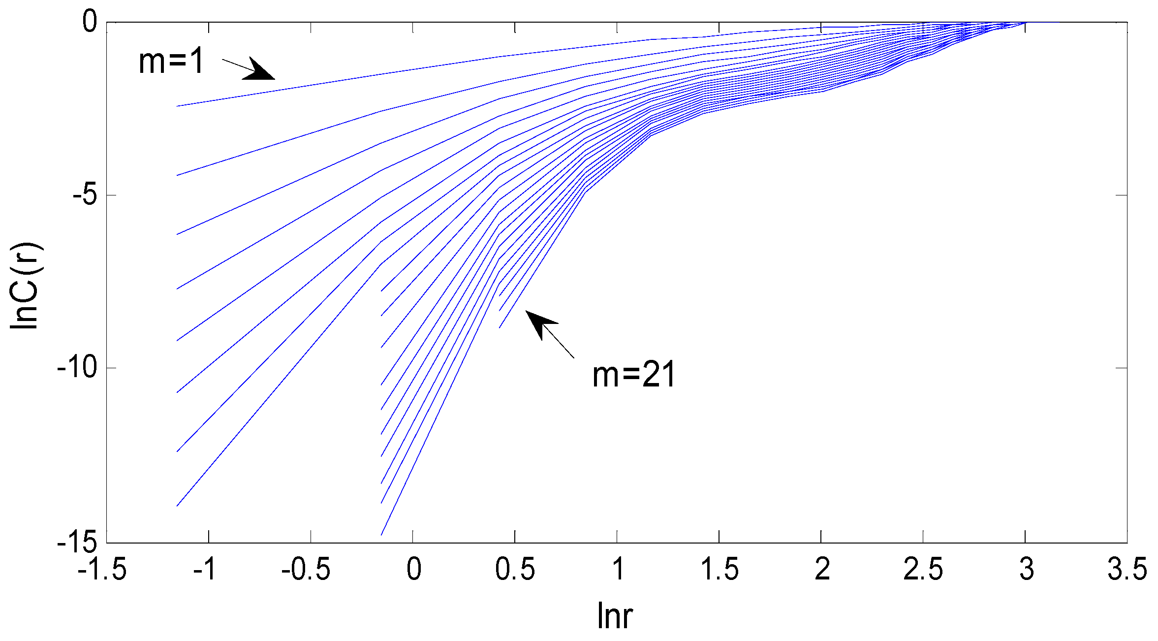
In chaos theory, all the possible states of a nonlinear chaotic system can be described by the phase space. Each point in phase space, called phase points, expresses the whole physical state [22]. PSR technique based on the Takens embedding theorem can recover the m-dimensional phase space or the structure of the attractor by single time series [23]. Thus, we can give a recurrence of the chaotic attractor in the original dynamical system and extract more quantity of the information from the limited dataset. This feature may increase the accuracy of modeling.

In this paper, the chaotic characteristics of WWTP are first analyzed and a new soft measurement method with PCA and ANN based on chaos theory is proposed for the prediction of BOD. Numerical experiments are designed to verify its effectiveness and feasibility by comparison between the ANN model with chaos theory and that without it.

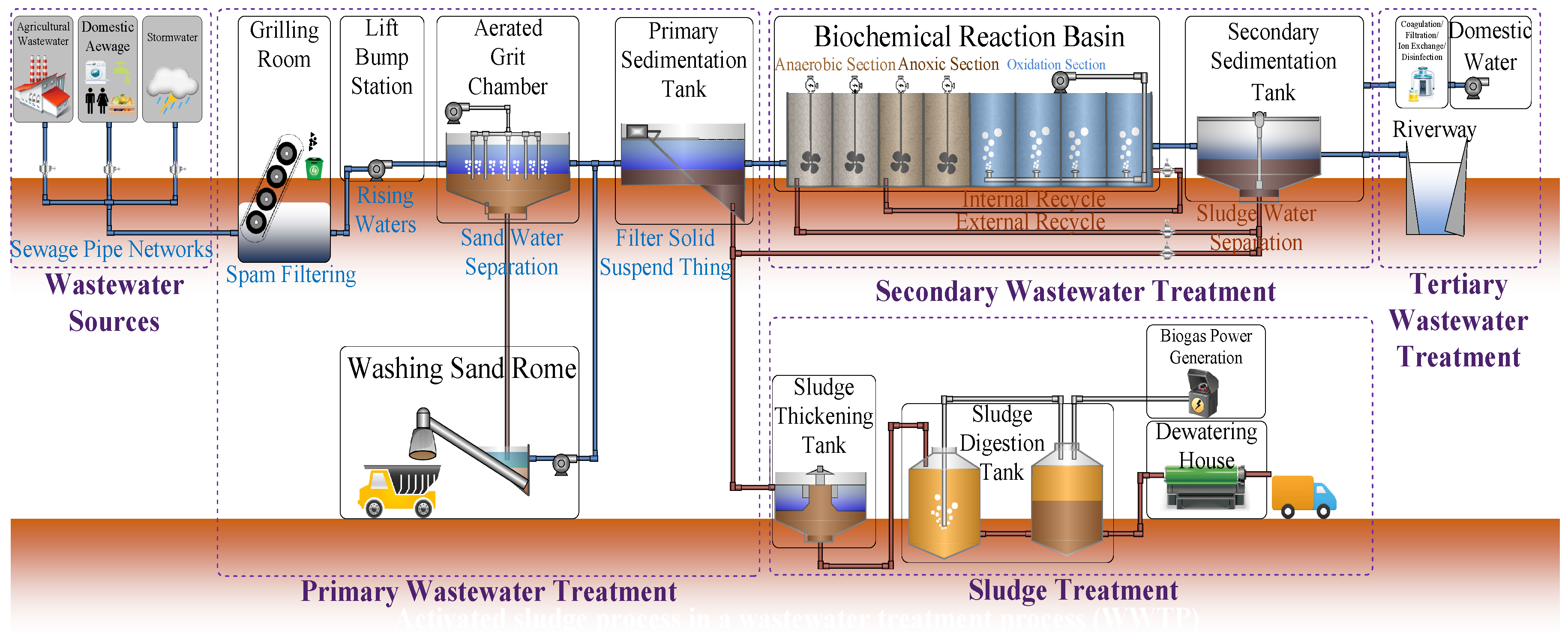
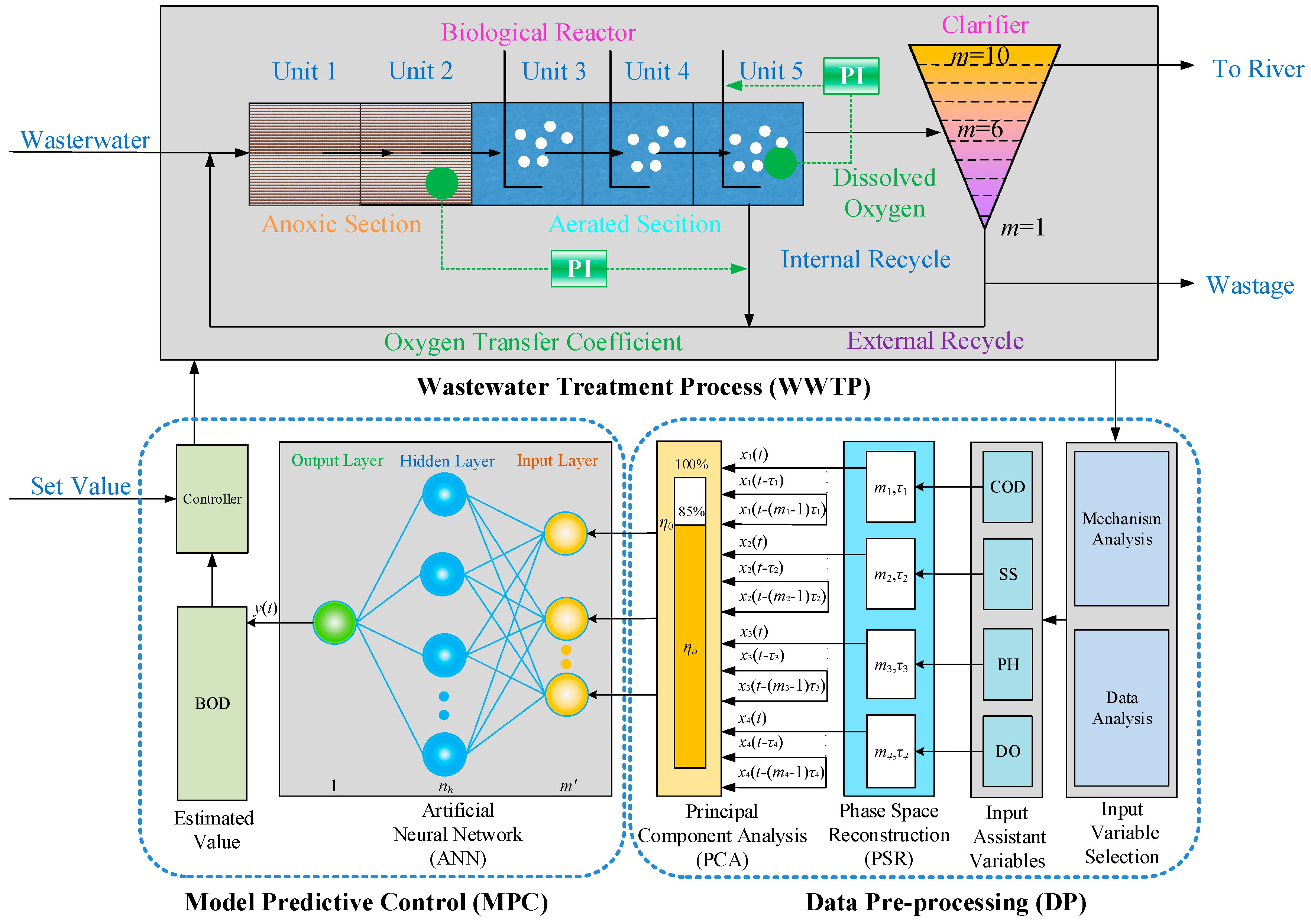
The rest of paper is organized as follows. In Section 2, the methods for chaotic characteristics analysis are introduced. PSR based on the Takens embedding theorem is presented for the univariate and multivariate time series modeling. The WWTP and the structure of the soft measurement prediction model for BOD based on PCA-ANN with chaos theory are described. In Section 3, the numerical experiments and the comparative results between the proposed method and other methods not based on chaos theory are presented. In Section 4, the several important factors which have effect on the prediction accuracy of the soft measurement modeling for effluent BOD based on chaos theory are analyzed and discussed. Finally, the conclusions are given in Section 5.

2. Methods

2.1. Chaotic Characteristic Analysis Methods

If the chaos theory is applied to soft measurement modeling in the WWTP, chaotic characteristics need to first be confirmed for WWTP. Correlation dimension (D), largest Lyapunov exponents (λ₁) and Kolmogorov entropy (K) are three characteristics to determine whether a dynamic system is chaotic or not [18]. Analysis methods for these characteristics are introduced in this section accordingly.

2.1.1. Phase Space Reconstruction (PSR)

Chaotic system cannot be predicted easily due to its features (e.g., initial value sensitivity, parameter sensitivity, ergodicity and random similarity) until the Takens embedding theorem was proposed by Takens in 1981. For the analysis of the characteristics of chaos, the key and first step is PSR based on the Takens embedding theorem which can recover the properties of the original dynamic system [23]. Then, an m-dimensional vectors can be obtained by reconstruction with a single time series observed from a chaotic system with two parameters which are delay time τ and embedding dimension m [24].

Suppose an observed univariate chaotic time series x(t) is generated by a nonlinear dynamic system. Based on the Takens embedding theorem, an m-dimensional embedding phase space point as input for the ANN model can be described as follows

$$X_i(t)={\left[x(t),x(t+\tau ),\cdots ,x(t+(m-1)\tau )\right]}^T,i=1,2,\cdots ,M$$

(1)

where m is embedding dimension, τ is delay time, M is the number of phase points, M = N − (m − 1), τ and N is the length of the observed time series. If m is large enough (m ≥ 2D + 1, D is the fractal dimension of the attractor), the reconstructed phase space is equivalent to the original dynamic system in the meaning of topology homeomorphism. There exists a smooth diffeomorphism f: R^m→R¹ as follows

$$x(t+(m-1)\tau +h)=f(X(t))$$

(2)

where h is the step of prediction. The reconstructed phase space X is composed of the M phase space points, then the formula is expanded as

$$X=\left(\begin{array}{cccc}x(1)\hfill & x(1+\tau )\hfill & \cdots & x(1+(m-1)\tau )\hfill \\ x(2)\hfill & x(2+\tau )\hfill & \cdots & x(2+(m-1)\tau )\hfill \\ ⋮& ⋮& ⋮& ⋮\\ x(M)\hfill & x(M+\tau )\hfill & \cdots & x(M+(m-1)\tau )\hfill \end{array}\right)$$

(3)

The output prediction vector Y can be descried by

$$Y={\left[x(1+(m-1)\tau )+h\cdots x(M+(m-1)\tau )+h\right]}^T$$

(4)

The above method for univariate chaotic time series can realize the single variable short-term prediction based on the history value [17,24,25,26]. It is worth noting that the soft measurement method is a multivariate modeling process. Moreover, multivariate chaotic time series modeling method contains more information associated with the original dynamic system which can improve the accuracy of prediction to some extent compared with the univariate chaotic time series modeling method [27,28,29].

For the multivariate chaotic time series prediction, suppose a given L-dimensional multivariate time series ${\left\{x_i(t)\right\}}_{t=1}^N={\left\{(x_1(t),x_2(t),\cdots ,x_L(t))\right\}}_{t=1}^N$. As in the case of univariate time series (when L = 1), the phase space points by PSR can be expressed as

$$\begin{array}{ll}\begin{array}{cc}\hfill V(t)=& [x_1(t),x_1(t+{\tau }_1),\cdots ,x_1(t+(m_1-1){\tau }_1),\hfill \\ & x_2(t),x_2(t+{\tau }_2),\cdots ,x_2(t+(m_2-1){\tau }_2),\hfill \\ & ⋮⋮⋮⋮\hfill \\ & x_L(t),x_L(t+{\tau }_L),\cdots ,x_L(t+(m_L-1){\tau }_L)]\hfill \end{array}& t=J_0,J_0+1,\cdots ,N;J_0=\underset{1\le i\le L}{\max }(m_i-1){\tau }_i+1\end{array}$$

(5)

where τ_i and m_i (i = 1, 2, …, L) are the ith variable’s delay time and the embedding dimensions, respectively. Based on Takens embedding theorem, the total embedding dimensions m = m₁ + m₂ + … + m_L. If m ≥ 2D + 1(D is the fractal dimension of the attractor) or each m_i is large enough, there exists an L-dimensional continued vector mapping F: R^m→R^m as follows

$$V(t+h)=F(V(t))$$

(6)

Equation (6) can be redefined by an L-dimensional continued vector mapping F_i: R^m→R, shown as

$$x_i(t+h)=F_i(v(t)),i=1,2,\cdots ,L$$

(7)

Then, the transformation from V_n to x_i,n+1 or V_n+1 reflects the evolutionary process from the current state to the future state for the original dynamic system, which signifies that the geometrical characteristics of the chaotic attractor in the reconstructed phase space are identical to the original state space. Thus, any differential or topological invariant quantities in the original dynamic system can be computed in the reconstructed phase space or reconstructed strange attractor. The value of the delay time τ_i and the embedding dimensions m_i can be determined by the following method.

(1) Delay Time

The delay time τ decides the quantity of information contained in the reconstructed phase space. In order to select an appropriate delay time τ, there are several methods to choose from, such as mutual information (MI) [17], autocorrelation function [25] and C-C method [30]. Because it can reflect the nonlinear correlation between the two time series, MI method is adopted broadly.

MI is a concept from the information theory. MI between x(t) and x(t + τ) is described by

$$I(\tau )={\displaystyle \sum _{t=0}^{N-\tau }p(x(t),}x(t+\tau )){\log }_2\left[\frac{p(x(t),x(t+\tau ))}{p(x(t))p(x(t+\tau ))}\right]$$

(8)

where N is the length of the observed time series, τ is delay time, p(x(t)) is the marginal probability density function (PDF) of x(t), p(x(t + τ)) is the marginal PDF of x(t + τ), and p(x(t),x(t + τ)) is the joint PDF of x(t) and x(t + τ). The optimal delay time τ is determined by the first minimum value of I(τ). As one of the methods to compute I(τ), the histogram-based MI estimation divides the x(t) − x(t + τ) coordinate space into (k_x(t) × k_x(t+τ)) equally sized (∆_x(t) × ∆_x(t+τ)) cells [31]. k_x is the number of cells, and it is selected by

$$k_x=round\left\{\frac{\zeta }{6}+\frac{2}{3\zeta }+\frac{1}{3}\right\}$$

(9)

$$\zeta =\sqrt[3]{8+324N+12\sqrt{36N+729N^2}}$$

(10)

where ζ is a constant value, and round{} means the closest integer of a real variable. Equations (9) and (10) are defined in reference [31] which has demonstrated that the method to choose k_x can obtain more accurate MI.

(2) Embedding Dimension

The embedding dimension m is the other key parameter for PSR. Many methods, such as false nearest neighbor method [20], G-P algorithm [32,33] and Cao’s method [34], are proposed to estimate the value of embedding dimension m. In this paper, we only need to obtain the minimum embedding dimension m_min based on the Takens embedding theorem [24,25,26,27,28,29]. The G-P algorithm proposed by Grassberger and Procaccia is adopted to determine it due to its easy calculation and good performance. The G-P algorithm is in detail as follows:

Step 1: The m is set to 2 as the initialization after the delay time τ has been obtained based on Section 2.1.1 (1). Further, M phase points can be generated by Equation (1). The correlation integral C_m(r) is the percentage of the number of the distance between each two phase points less than r in all phase points [35]. C_m(r) can be calculated by

$$C_m(r)=\underset{r\to \infty }{\lim }\frac{2}{M(M-1)}{\displaystyle \sum _{i=1}^M{\displaystyle \sum _{j=i+1}^{M}H(r-\Vert X_i-X_j\Vert )}},i\ne j$$

(11)

where r is the given radius (r $\in$ {r_min, r_min + δ, r_min + 2δ, …, r_max}), ‖X_i − X_j‖ is the Euclidean distance between phase space points X_i and X_j. H(x) is the Heaviside function defined as

$$H(x)=\{\begin{array}{l}1,x>0\\ 0,x<0\end{array}$$

(12)

In practical computation, r is computed by

$$r=r_{\min }+k\cdot \delta$$

(13)

$$\delta =\frac{r_{\max }-r_{\min }}{s}$$

(14)

where r_max = max‖X_i − X_j‖, r_min = min‖X_i − X_j‖ is the maximum and minimum of the ‖X_i − X_j‖, respectively. k is a variable (k = 0, 1, 2, …). δ is the step length of the r. s is the number of the points need to be inserted (s = 50~200). With the increasing of r, a curve of lnC_m(r)~lnr corresponding to one m is plotted by Equations (11)–(13).

Step 2: Multiple curves of lnC_m(r)~lnr can be plotted by different value of m. If the system is chaotic, C_m(r) is proportional to r^D2(m) which is described by

$$C_m(r)\propto r^{D_2(m)}or{D}_2(m)=\underset{r\to 0}{\lim }\frac{\ln C_m(r)}{\ln r}$$

(15)

where D₂(m) is correlation dimension with different embedding dimension m (m = 1, 2, …). D₂(m) is one of the attractor’s fractal dimension D which can be determined from the slope of the curve between lnC_m(r) and and lnr in the section of linearity.

Step 3: When D₂(m) tends to saturate with the increase of the embedding dimension m, the system is chaotic, and the value of the saturate gives D₂(m). The minimum embedding dimension m_min can be decided by the formula m ≥ 2D + 1 referred before. If not, the system is random.

2.1.2. Lyapunov Exponent

The Lyapunov exponents describe the phenomenon of dispersion for two nearby initial values due to the butterfly effect, and quantify the average exponential rates of divergence or convergence of adjacent trajectories in phase space [18,19,22].

For one-dimensional dynamic system x_n+1 = F(x_n), after the N steps’ iteration or evolution, the Lyapunov exponent λ is defined as

$$\lambda =\underset{N\to \infty }{\lim }\frac{1}{N}{\displaystyle \sum _{i=0}^{N-1}{\log }_2\left|\frac{dF(x)}{dx}\right|}$$

(16)

If the system contains one positive Lyapunov exponent, we can demonstrate the dynamic system is chaotic [19]: (a) when λ ≤ 0, the system is stable; (b) when 0 < λ < ∞, the system is chaotic; and (c) when λ = ∞, the system is random. Therefore, only the Largest Lyapunov Exponent (LLE), denoted as λ₁, needs to be calculated. In our study, the Wolf algorithm [19,36] is used to obtain the LLE.

2.1.3. Kolmogorov Entropy

Kolmogorov entropy (K) measures the degree of chaos for a nonlinear system. The more the loss ratio of the information for the system, the larger the value of K. And the loss ratio of the information is proportional to the level of the chaos for the dynamical system [18,21].

For an n-dimensional dynamic system, assume that the n-dimensional phase space is divided into boxes of size rⁿ. We make an assumption that the system has a strange attractor and x(t) is its pathway. If p(i₀, i₁, …, i_d) is the joint probability that t = τ in box i₁, t = 2τ in box i₂, ..., and t = dτ in box i_d, K is defined by

$$K=-\underset{\tau \to 0}{\lim }\underset{r\to 0}{\lim }\underset{d\to \infty }{\lim }\frac{1}{d\tau }{\displaystyle \sum _{i_0,\cdots ,i_d}p(i_0,\cdots ,i_d)}\ln p(i_0,\cdots ,i_d)$$

(17)

where τ is delay time, and r is the edge length of the boxes. But, the process of the computation for K based on the above formula is too cumbersome. For this reason, the G-P algorithm [37] is applied to reduce the computation complexity. In this method, K can be estimated by the value of K₂ which is stable with the growth of m. The K₂ is described by

$$K_2=\frac{1}{\tau }\ln \frac{C_m(r)}{C_{m+1}(r)},(r\to 0,m\to \infty )$$

(18)

where m is the embedding dimension, and C(r) is the correlation integral. Different K represent different states of the motion [18]: (a) K = 0 means regular motion; (b) 0 < K < ∞ means chaotic motion; (c) K = ∞ means random motion.

2.2. Soft Measurement Model

2.2.1. Wastewater Treatment Plant (WWTP)

WWTP plays an important role in the reclamation and recycling of sewage. The activated sludge process as shown in Figure 1 is a common and effective technique to realize the WWTP. The activated sludge contains various micropopulation which can eliminate and defuse the harmful substances for the human and ecological environment. Generally, WWTP consists of four parts which are primary stage (physical treatment), secondary stage (biological treatment and secondary sedimentation tank), tertiary stage (advanced treatment) and sludge treatment, which are described in details as follows [9,38]:

(a)

Primary treatment. The preliminary step is used to remove large objects that have negatively influence on downstream processing equipment, the sand and other solid waste from the influent wastewater. Dense organic material is removed through primary sedimentation tank. The primary treated wastewater is transported to the biochemical reaction basin.

(b)

Secondary treatment. The biological treatment takes place in biochemical reaction basin in which the organic carbon (C), biological nitrogen (N), biological phosphorus (P) and ammonium are removed from the liquid portion of the wastewater by microorganism in the activated sludge and transferred to the solids portion. There is the secondary sedimentation tank, in which the treated water and the sludge are separated by physical subsiding.

(c)

Tertiary treatment. The advanced treatment further removes the refractory organic matter and soluble inorganic matter in order to make potable water when it is needed.

(d)

Sludge treatment. A fraction of the separated sludge in secondary sedimentation tank is returned to the biochemical reaction basin to sustain the ability of the wastewater treatment. The other redundant sludge is carried away after sludge treatment process.

WWTP is a complex nonlinear dynamic process due to its multivariable coupling, unstable, large-scale disturbances and other uncertain human and environmental factors [1,2]. These characters bring great challenges to the system modeling, controlling and parameter prediction. For the modeling of WWTP, there are two main segments that are (1) the hydraulic model and (2) the biological model. The hydraulic model is used to describe the flow and technological processes. The biological model, which is the main component of the WWTP, shows the behavior and effects of the activated sludge. The biological process is mainly related to the activated sludge and it represents microbial growth, death, and nutrient consumption. These activated sludge models are used to approach enormous amount of biological processes which occurred in each bioreactor [38]. Overall, the modeling of the WWTP is still a complicated problem for the complex and changing process [16]. Due to the limitations of technology and chemical factors, some key water quality and environmental parameters cannot be measured easily and accurately [38]. The practical WWTP also is unstable and time-varying with the interaction of the variables with each other and disturbance [15]. Hence, the modeling is a challenging task so that accurate models are researched for describing WWTP.

2.2.2. Principal Component Analysis (PCA)

Principal Component Analysis (PCA) is an important feature extraction method for multivariate statistical analysis [11,12,27]. It can express datasets by effective characteristics with fewer dimensions while maintaining the quantity of the information in time series.

In fact, PSR increases the dimensions of the input assistant variables to obtain more information hidden in the chaotic dynamic system [24,25,26,27,28,29]. Using PCA, we can reduce the dimensions of the input assistant variables without information loss to enhance the ability of generalization performance and to avoid over-fitting on account of overmuch input dimensions on the basis of PSR [27]. In this paper, PCA is used to reduce the dimensions after the PSR and before the modeling task.

The basic steps of PCA are as follows:

Suppose the input sample matrix X_M×m, where m = m₁ + m₂ + … + m_L, and M = N − max[(m_i − 1) × τ_i]. m_i and τ_i (i = 1, 2, …, L), are the ith input variable’s embedding dimension and delay time, respectively.

Step 1: Standardize the X_M×m into ${\tilde{X}}_{M\times m}$:

$${\tilde{x}}_{ij}=\frac{x_{ij}-{\overline{x}}_j}{{\sigma }_j}$$

(19)

where i is the number of phase points, i = 1, 2, …, M; j is the dimension of phase points, j = 1, 2, …, m; x_ij is the jth dimension of ith phase points; ${\overline{x}}_j$ is the mean of jth dimension of phase points; σ_j is the standard deviation of jth dimension of phase points.

Step 2: Calculate the covariance matrix of ${\tilde{X}}_{M\times m}$:

$${\psi }_x=E(\mathit{x}{\mathit{x}}^T)=\frac{1}{M}{\tilde{X}}_{M\times m}^T{\tilde{X}}_{M\times m}$$

(20)

Step 3: Eigenvalue and its corresponding orthonormal eigenvector of ${\psi }_x$ are obtained as λ₁ ≥ λ₂ ≥ … ≥ λ_a ≥ 0 and p₁, p₂, …, p_a, respectively.

Step 4: Compute the principal component (or score) t_i:

$$t_i={\mathit{p}}_i^T\mathit{x}=p_{i1}{x}_1+p_{i2}{x}_2+\cdots +p_{im}{x}_m,i=1,2,\cdots ,a$$

(21)

Step 5: The covariance matrix ψ_x is made up of m eigenvectors, and only the first a eigenvectors corresponding to larger eigenvalues are reserved. Thus, the number of the remaining eigenvectors is (m − a) with related smaller eigenvalues, and they are filtered out, due to being regarded as noise. Because the existing diversified methods lead to different results, how many smaller eigenvalues should be abandoned to obtain the best results, is a difficult problem. The appropriate number of principal components can filter out most of the noise and acquire the best structure of data. In this paper, a simple and classical method is adopted.

The contribution rate of variance δ_i for t_i is defined as

$${\delta }_i=\frac{{\lambda }_i}{{\displaystyle \sum _{j=1}^m{\lambda }_j}}$$

(22)

The contribution rate of the accumulated variance η_a for the first a principal component is then described by

$${\eta }_a={\displaystyle \sum _{i=1}^a{\delta }_i}=\frac{{\displaystyle \sum _{j=1}^a{\lambda }_i}}{{\displaystyle \sum _{i=1}^m{\lambda }_i}},a\le m$$

(23)

The number of principal components can be determined based on the pre-set contribution rate of accumulated variance η₀ (such as 85%). The minimum a satisfying η_a > η₀ is then the acquired value.

2.2.3. Multivariate Chaotic Time Series Model for BOD

In this paper, the structure of the soft measurement model based on chaos theory with PCA-ANN for effluent BOD is shown in Figure 2. The data which are measured in WWTP are sent to the data pre-processing (DP) module. The input assistant variables are determined by the mechanism and data analysis, which are easily measured, economical and have greater chemical correlation with effluent BOD. According to the analysis and existing papers [1,2,4,5,13], influent COD, SS, pH and DO are selected as the input assistant variables finally.

Before modeling, the input and output data are preprocessed by

$$x^{\prime }=(v_{\max }-v_{\min })\times \frac{x-x_{\min }}{x_{\max }-x_{\min }}+v_{\min }$$

(24)

where x is the original observed value, $x^{\prime }$ is the normalized value, x_max and x_min are the maximum and minimum of the original observed value, respectively; and v_max and v_min are the maximum and minimum of the normalized value, respectively. In this paper, we set v_max = 1, v_min = −1, and the experiment data are all normalized into [−1, 1].

The existing soft measurement models all adopt the easy-measured variables to be input directly without taking the chaotic characteristic of WWTP into consideration. In addition, the PSR technique can recover the structure of the chaotic attractor under the condition that the WWTP is demonstrated to be a chaotic system. This will increase the information of the nonlinear dynamic system based on the analysis of Section 2.1.

The soft measurement model with multivariate chaotic time series is established based on the Section 2.1.1, where the step of prediction h is set to zero. The variable COD, pH, SS, DO are taken as the inputs of the ANN. The dimension of input assistant variables is extended by PSR based on calculated delay time τ and embedding dimension m. The corresponding BOD is regarded as the output. Before entering into the ANN, the dimension of reconstructed input variable are reduced by PCA. The mapping relation can be descried as

$$\begin{array}{l}BOD(t+(m_{BOD}-1){\tau }_{BOD})=\\ f(COD(t),COD(t+{\tau }_{COD}),\cdots ,COD(t+(m_{COD}-1){\tau }_{COD}),\\ PH(t),PH(t+{\tau }_{PH}),\cdots ,PH(t+(m_{PH}-1){\tau }_{PH}),\\ SS(t),SS(t+{\tau }_{SS}),\cdots ,SS(t+(m_{SS}-1){\tau }_{SS}),\\ DO(t),DO(t+{\tau }_{DO}),\cdots ,DO(t+(m_{DO}-1){\tau }_{DO}))\end{array}$$

(25)

Based on the multivariate chaotic time series prediction method in Section 2.1.1, the input variables are reconstructed with m_i and τ_i (i = 1, 2, …, L) by PSR. Then, each input variable generates M m_i-dimensional phase points. The input dimensions have been changed from L to m (m = m₁ + m₂ + … + m_L). In order to enhance the ability of generalization performance and avoid over-fitting on account of overmuch input dimensions, the PCA technique in Section 2.2.2 is adopted to reduce the input dimensions to $m^{\prime }$ without information loss. Afterwards, the obtained inputs are taken as the inputs of ANN. And the number of neurons in the hidden layers can be estimated by [18]

$$n_h=\sqrt{m^{\prime }+1}+\alpha$$

(26)

where $m^{\prime }$ is the input dimensions, and α is an integer (α $\in$ [1, 10]). Hence, the structure of the ANN is $m^{\prime }$ − n_h − 1. The multivariate chaotic time series prediction method is only suitable for the chaotic time series. If the method is applied for the soft measurement modeling, the chaotic characteristic of input and output variables time series need to be demonstrated and analyzed first.

The ANN can map the function f (·) by training with the input and output dataset. In practical engineering applications, the processed data are taken as the input of ANN for model predictive control (MPC) [39]. As the output of ANN, the estimated BOD values are compared with the set values. The difference value is used as the control signal for controller. The method not only accomplishes the soft measurement, but also takes the chaotic information into consideration.

2.2.4. Evaluation of the Model

The sum of squared error (SSE) is chosen as the training target function which can be defined by

$$\mathrm{SSE}={\displaystyle \sum _{i=1}^N}{(y_i-{\widehat{y}}_i)}^2$$

(27)

where $y_i$, ${\widehat{y}}_i$, and N are the measured values, the predicted values, and the length of the measured values, respectively. And root mean squared error (RMSE) and mean absolute percentage error (MAPE) are used to evaluate the prediction accuracy and effectiveness of the proposed prediction model and other models [8]. They are calculated as follows:

$$\mathrm{RMSE}=\sqrt{\frac{1}{N}{\displaystyle \sum _{i=1}^N{(y_i-{\widehat{y}}_i)}^2}}$$

(28)

$$\mathrm{MAPE}=\frac{1}{N}{\displaystyle \sum _{i=1}^N\left|\frac{y_i-{\widehat{y}}_i}{y_i}\right|}\times 100\%$$

(29)

The RMSE reflects the degree of the discrepancy between the predicted and the measured values. The MAPE reflects the mean of the absolute percentage error of prediction.

3. Results

3.1. Data Source

The 609 data are derived from a real wastewater treatment plant every day from 1 January 2011 to 31 August 2012 in Beijing as shown in Figure 3.

In Figure 3, the original data contains some outlier data or noise which have impact on the chaotic characteristic analysis. The noise points are usually generated by instruments, manual operation, other unforeseen circumstances, etc. The values of noise are also random and abnormal. As a phenomenon found in non-linear dynamic system, chaos is deterministic and random-like. The denoised data changes within a definite range and doesn’t contain the outlier data or missing data. Experiment data are 598 points in total after noise elimination with 3σ-rule. Influent COD, SS, pH and DO, which are measured in aeration tank, are taken as the inputs. Effluent BOD is used as the output for the soft measurement model.

3.2. The Chaotic Characteristic of WWTP

The chaotic characteristics of WWTP are first analyzed to further decide whether the soft measurement model can be designed based on chaos theory. The G-P algorithm is adopted to calculate the minimum embedding dimension m_min based on Takens embedding theorem for PSR. Before application of the PSR, the optimal delay time τ of BOD is computed by MI (Section 2.1.1). The results are shown in Figure 4.

From Figure 4, we can see the optimal delay time τ is 2 for the time series of BOD and corresponding I(τ) is 1.8377, which means that MI reaches the first minimum in the second day. The curves of lnr—lnC(r) for different embedding dimensions m from 1 to 21 are drawn as shown in Figure 5 after the delay time τ has been determined.

In Figure 5, the slope of each curve which is calculated by linear fitting in the non-scaling interval is the correlation dimension D for different embedding dimensions m. Based on the results in Figure 5, the curves of D over m for BOD can be plotted in Figure 6.

As one can see from Figure 6, even though the correlation dimension D increases with the increasing embedding dimension m, it approaches to a saturation value (namely saturated correlation dimension) 1.2114 when m ≥ 8. Then the minimum embedding dimension m_min for the time series of BOD is 8 based on the Figure 6 and the principle of the m ≥ 2D + 1 (Section 2.1.1). The fractional correlation dimension D reveals that the BOD time series may be chaotic.

After the determination of the delay time τ and embedding dimension m, the phase space can be reconstructed based on the PSR approach. The two-dimensional phase space portrait is reconstructed by the BOD time series as shown in Figure 7. According to Figure 7, the two-dimensional phase space portrait shows an obvious attractor in the reconstructed phase space. This phenomenon or motion feature, which seems to have a certain regularity, is different from a random motion.

However, we cannot yet conclude that the evolution process of BOD must be chaotic. To further judge the characteristics of the BOD time series, the Kolmogorov entropy (K), LLE (λ₁) are calculated by the G-P algorithm (Section 2.1.3) and Wolf algorithm (Section 2.1.2), respectively. The value of K is 0.067637 (K > 0) in Figure 8. Besides, the LLE λ₁ is 0.31441 (λ₁ > 0). K and λ₁ are all positive which demonstrates that the BOD time series in WWTP is chaotic.

From the previous analysis, we can demonstrate that the effluent BOD time series is chaotic, that is, the wastewater treatment system is chaotic. In order to further verify the result, more variables need to be tested. Therefore, the COD, pH, SS and DO time series are analyzed by the same processes and method in Section 2.1. The results are listed in

Table 2. Delay time τ, correlation dimension D, embedding dimension m, Kolmogorov entropy K, largest Lyapunov exponent λ₁ of the BOD, COD, pH, SS, DO.

	τ	D	m	K	λ1
BOD	2	1.2114	8	0.067637	0.31441
COD	3	1.5542	6	0.025344	0.16525
pH	5	2.1654	6	0.050063	0.21736
SS	3	1.3760	5	0.043527	0.59079
DO	5	2.7908	7	0.079561	0.70781

.

The results in Table 2 have two functions as follows: (1) whether the dynamic system is chaotic or not can be judged based on the value of m, K, λ₁; (2) the necessary parameters (i.e., m and τ) for multivariate chaotic time series modeling are provided.

The analysis experiments show that the BOD time series and other variables in WWTP all have fractional correlation dimension, positive K and λ₁. It is testified that the random-like motion of the various WWTP time series can be explained as a chaotic phenomenon. After the chaotic characteristics analysis, the chaotic time series prediction methods can be applied to the modeling of the soft measurement of BOD.

3.3. Soft Measurement for BOD Based on Chaos Theory

Based on Table 2 and Section 2.2.2, the variance explained by the sorted principal components are shown in Figure 9.

The histogram represents the variance explained (or the contribution rate of variance) by each principal component. The blue curve represents the total variance explained. One can see that the total variance explained is 86.10% (>85%) by adding the first 14 principal components.

From Table 2, the number of neurons in the input layer is determined by the embedding dimensions m, which is 24. Then the input dimensions are reduced to 14 based on the results of the PCA technique in Figure 9. To compare different models, we set the number of the input and hidden neurons for all models to 14 and 10 or 12 based on Figure 9 and Equation (26), respectively. And the learning rate is set to 0.0045. The maximum training error is set to 0.001, and the maximum iterations to 5000.

Then, 568 phase points are generated from the 598 measured data based on the Equations (1) and (5) by PSR. Thus, the beginning of the prediction is the 31st time series point according to Equation (5). The first 368 phase points are taken as training data, and the remaining 200 phase points are used as testing data. Fuzzy neural network (FNN) is adopted for soft measurement modeling for BOD. In order to verify the performance of the model with the chaos theory, the FNN with chaos theory (C-FNN) are applied for the prediction of BOD as well. The training and testing output of the FNN, C-FNN for BOD are shown in Figure 10 and Figure 11, respectively. The scatter plots of the training and testing errors against the measured values are shown in Figure 12 and Figure 13, respectively.

Based on Figure 10, Figure 11, Figure 12 and Figure 13 and

Table 3. The performance comparison of different models.

Model	m	τ	nh	Training RMSE (mg/L)	Testing RMSE (mg/L)	MAPE (%)		Run Time (s)
						Min	Max
MLP [14]	[1 1 1 1 1]	——	12	0.4372	1.0799	9.29%	12.45%	70.85
C-MLP	[8 6 6 5 7]	[2 3 5 3 5]	12	0.5104	0.7181	5.85%	8.45%	74.82
RBF [7]	[1 1 1 1 1]	——	12	0.5981	0.8504	8.33%	9.15%	64.38
C-RBF	[8 6 6 5 7]	[2 3 5 3 5]	12	0.3013	0.5830	5.12%	6.70%	83.98
Elman	[1 1 1 1 1]	——	10	0.4885	0.7810	7.40%	8.79%	184.76
C-Elman	[8 6 6 5 7]	[2 3 5 3 5]	10	0.1947	0.5493	4.42%	6.38%	202.23
FNN [1]	[1 1 1 1 1]	——	10	0.3665	0.6528	5.94%	7.68%	716.68
C-FNN	[8 6 6 5 7]	[2 3 5 3 5]	10	0.1356	0.3430	2.90%	5.40%	824.24

Notes: n_h, the number of the hidden neurons; ——, without PSR.

, the calculated training and testing RMSE, the minimum and maximum MAPE of FNN are 0.3665 and 0.6528, 5.9424% and 7.6864%, respectively. As a comparison, the training and testing RMSE, the minimum and maximum MAPE of C-FNN are 0.1356 and 0.3430, 2.9023% and 5.4033%, respectively. We can see that the C-FNN has better accuracy than FNN based on the value of the training or testing RMSE and MAPE. Besides, C-FNN has the smaller errors and more stable performance than FNN from the scatter plots in Figure 12 and Figure 13, especially in extreme points.

In order to further verify the effects of the models which take chaos theory into consideration, the corresponding results and performance comparison of different models are also listed in Table 3. When m = [1 1 1 1 1] with each element representing BOD, COD, pH, SS and DO, respectively, it means that the input variables cannot be reconstructed based on Equations (3) and (4). When m = [8 6 6 5 7], it means that the input variables are reconstructed as shown in Table 3. The neural network model with chaos theory is written as C-ANN. The ANNs which are used for comparison include multilayer perceptron (MLP) [14], radial basis function neural network (RBF) [7], Elman neural network (Elman), fuzzy neural network (FNN) [1], MLP with chaos theory (C-MLP), RBF with chaos theory (C-RBF), Elman with chaos theory (C-Elman), and FNN with chaos theory (C-FNN). All ANNs adopt the traditional gradient descent method for training all connection weights.

From Table 3, the C-ANNs all have smaller testing RMSE and MAPE than the corresponding ANN without chaos theory. In terms of the MAPE, the accuracy of the models with chaos theory increases about 2%–4% compared with the corresponding ANN without chaos theory.

4. Discussion

The WWTP has been proven to be a chaotic system based on Section 3.2. The PSR technique in chaos theory can improve the accuracy of soft measurement modeling for BOD based on the results of the Table 3 in Section 3.3. That is because we can obtain a good representation of the attractor of the dynamical system by PSR [19]. Therefore, it provided more information than the corresponding model without chaos theory. Then, ANN can learn more accurate laws from the richer information through training. In the practical application, the input and output data are obtained from measuring instruments or laboratory, which are memorized as the history data. Then, the datasets are analyzed and computed for chaotic characteristic and modeling for BOD. After it, the value of BOD can be obtained with the current input datasets. Actually, several important factors have great effects on the prediction accuracy of the soft measurement modeling for BOD based on chaos theory:

(a)

The quantity of the original dataset. On the one hand, the more the amount of data, the more dynamic information can be contained and the better precision the chaotic characteristic analysis has. On the other hand, the ANN can learn more relationship and disciplinarian between input and output from it.

(b)

Effects of noise in the data. Generally, the original data also contain some noise, which have a negative effect on chaotic characteristic analysis and modeling in some degree. The noise can be defined as the unexplainable or random data that is found within the given data. In order to compare the difference between the de-noised data (Table 2) and noisy data for the chaotic characteristic analysis, the experiment are designed for noisy data. The results are listed in

Table 4. Delay time τ, correlation dimension D, embedding dimension m, Kolmogorov entropy K, largest Lyapunov exponent λ₁ of the BOD, COD, pH, SS, DO for noisy data.

	τ	D	m	K	λ1
BOD	9↑	—	—	0.117459↑	—
COD	8↑	—	—	0.050545↑	0.31656↑
pH	6↑	2.0546↓	5↓	0.052154↑	0.28380↑
SS	2↓	4.1697↑	9↑	—	0.85217↑
DO	3↓	—	—	0.126237↑	1.47943↑

Notes: ↑, increase; ↓, decrease; —, default.

.

Table 4 shows that the data without noise-removal processing have great influence on the chaotic characteristics analysis. The existence of the noisy data can cause the increasing of the K, as well as λ₁. This phenomenon is consistent with the significance of the K and λ₁ in Section 2.1.2 and Section 2.1.3. Moreover, it further misguides the chaotic characteristics analysis (i.e., some nonlinear dynamic system which is not chaos may be regarded as a chaotic system).

Some of τ, D, m, K, λ₁ cannot be obtained under the influence of noise by the method mentioned in Section 2.1. The noisy data made it harder to obtain reliable parameters for modeling. According to the change of τ, D, m from Table 2, Table 3 and Table 4, the noise has different influence on various water quality parameters. Therefore, noise-removal processing is a necessary step.

(c)

The selection of the input variables. Different input variables will lead to different results. With mechanism analysis, simulation study and existing papers [1,2,4,5], influent COD, SS, pH and DO are selected as the input assistant variables finally. For more comprehensive analysis, the other models with different input variables have been examined for comparison and selection. The testing RMSE of soft measurement modeling for BOD with different input variables are shown in

Table 5. The testing RMSE of soft measurement modeling for effluent BOD with different input variables.

Inputs	MLP [14]	C-MLP	RBF [7]	C-RBF	Elman	C-Elman	FNN [1]	C-FNN
(1)	1.3284	0.8791	0.9423	0.6842	0.8641	0.7281	0.8415	0.6756
(2)	1.1746	0.6926	0.8615	0.6028	0.7755	0.5807	0.6514	0.3718
(3)	1.0799	0.7181	0.8504	0.5830	0.7810	0.5493	0.6528	0.3430
(4)	1.5440	1.2125	1.3352	0.9647	1.1434	0.8542	0.9542	0.7654
(5)	2.0158	1.6452	1.5434	1.1715	1.3682	0.9156	1.3105	1.0426
(6)	3.5415	3.0571	3.1642	2.4546	2.5674	2.3482	2.6461	2.4875

Notes: (1): COD, pH, SS, DO, T, ORP; (2): COD, pH, SS, DO, T; (3): COD, pH, SS, DO; (4): pH, SS, DO; (5): pH, DO, T; (6): pH, DO. The best testing RMSE are marked in bold.

.

From Table 5, the model with only pH and DO as the input has the lowest accuracy. Though the pH and DO can be measured online, the information that is provided by only pH and DO is insufficient for prediction. The models with three input variables (i.e., pH, DO, T and pH, SS, DO) have better performance than the model with only pH and DO since the more information come from the T or SS. The model with COD, pH, SS and DO as the inputs has the best accuracy among the given models. It is worth mentioning that the model with COD, pH, SS, DO and T has similar performance with COD, pH, SS and DO. However, the model with COD, pH, SS and DO is selected in this paper due to the fewer inputs and better accuracy. In addition, the model with five input variables (i.e., COD, pH, SS, DO, T, and ORP) does not have better precision by reason of the increasing dimensions of inputs, which have a negative effect on ANN’s generalization. Therefore, the multiple factors such as biochemical mechanism, the number of inputs, accuracy, etc. need to be considered for the choice of input variables.

(d)

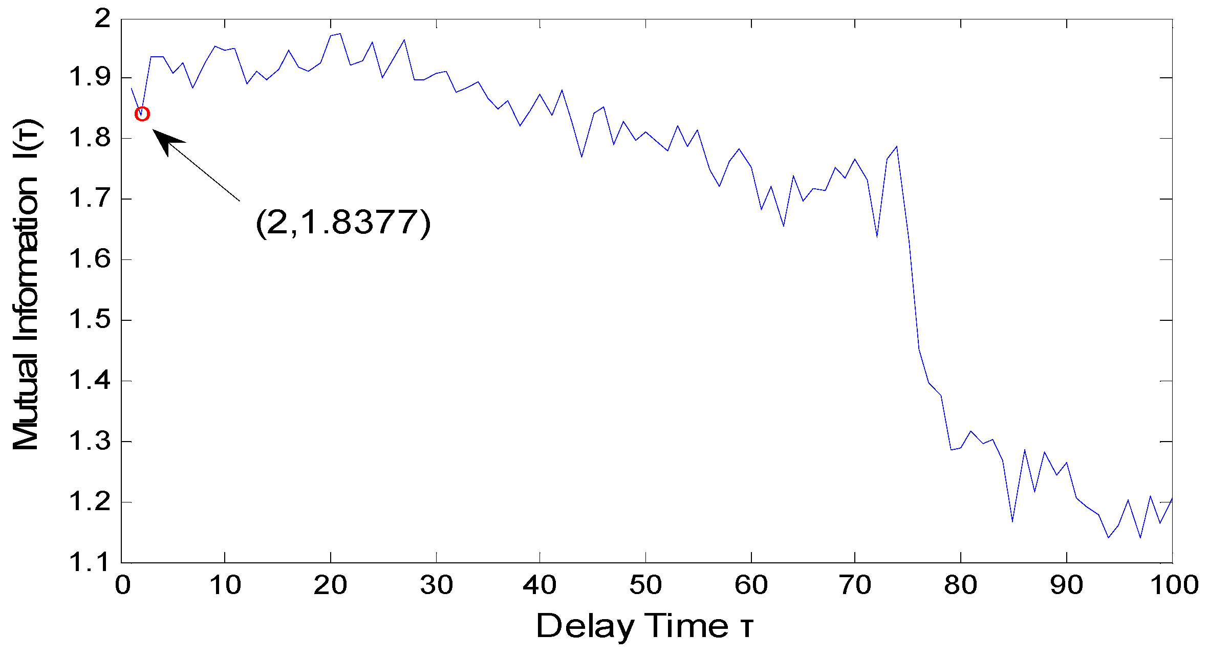
The accuracy and rationality of the chaotic characteristic parameters. The chaotic characteristic parameters include delay time τ, embedding dimension m, Kolmogorov entropy K, and largest Lyapunov exponent λ₁. The m, K and λ₁ are used to judge whether the nonlinear system is chaotic or not and indicate the degree of chaotic motion. The K and λ₁, which just are the characterization of chaos, can provide key information for judging chaotic system and have no impact on the modeling or prediction. Especially, τ and m, which directly decide the reconstructed phase space by PSR, need to be appropriately selected. The performance comparison with different τ and m for C-FNN model are listed in

Table 6. The performance comparison with different τ and m for C-FNN model.

m	τ	nh	M	Mtrain	Mtest	Training RMSE (mg/L)	Testing RMSE (mg/L)	MAPE (%)
								Min	Max
[9 9 9 9 9]	[2 3 5 3 5]	10	558	342	200	0.2935	0.4976	4.18%	7.41%
[8 8 8 8 8]	[2 3 5 3 5]	10	563	342	200	0.1961	0.4224	3.56%	6.85%
[5 5 5 5 5]	[2 3 5 3 5]	10	578	342	200	0.1780	0.3973	3.29%	6.03%
[1 1 1 1 1]	[2 3 5 3 5]	10	598	342	200	1.1683	1.5390	13.44%	15.42%
[8 6 6 5 7]	[2 3 5 3 5]	10	568	342	200	0.1404	0.3622	2.98%	5.68%
[8 6 6 5 7]	[1 1 1 1 1]	10	591	342	200	0.4862	0.7493	6.23%	9.97%
[8 6 6 5 7]	[2 2 2 2 2]	10	584	342	200	0.2698	0.4735	4.07%	7.64%
[8 6 6 5 7]	[5 5 5 5 5]	10	563	342	200	0.2120	0.4476	3.75%	5.28%
[8 6 6 5 7]	[8 8 8 8 8]	10	542 *	342	200	0.7503	1.1023	9.56%	12.31%

Notes: M, the number of phase points; M_train, the number of training data; M_test, the number of testing data; * the number of experimental phase points.

. The choice of this paper for τ and m are marked in bold. The number of the experimental phase points is the minimum value among them.

The accuracy of the modeling or prediction appeared downward trend with the increase or decrease of τ and m on the basic of the results in Table 2. This not only proved that the calculated value of the τ and m were accurate and reasonable, but also indicated that too large or too small values of τ and m can lead to poor prediction performance. Therefore, the estimation and calculation of the chaotic characteristic parameters is a very important part of the identification and modeling.

(e)

The selection of the ANN modeling parameters. The ANN modeling parameters include the number of input and hidden neurons, learning rate, maximum iterations, and maximum training error. The number of inputs is determined by the embedding dimension m and PCA. Several experiments are conducted for the number of hidden neurons based on the errors and the range in Equation (26). The larger or smaller learning rate can cause the oscillation or slower convergence speed for ANN, respectively.

(f)

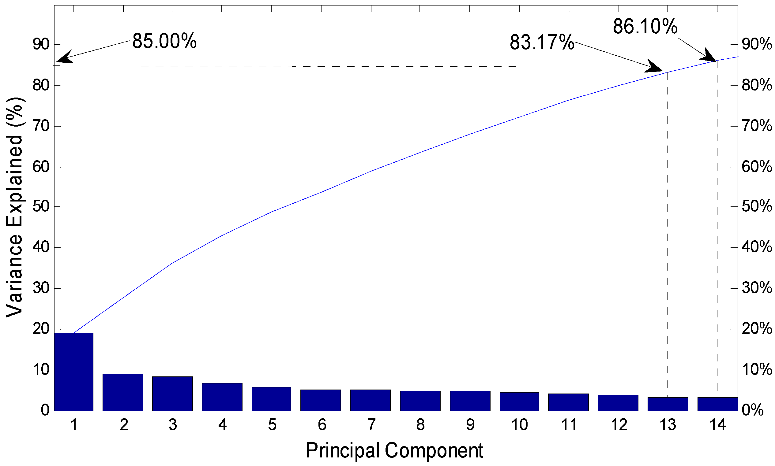
Normalization and dimensionality reduction. Generally, the scope of the normalization is [0, 1] or [−1, 1]. The input and output dataset all need to be normalized for better training performance and generalization ability. The dimensions of input variables should be reduced for higher data quality. This needs to be further analyzed and tested for reasonable choice.

5. Conclusions

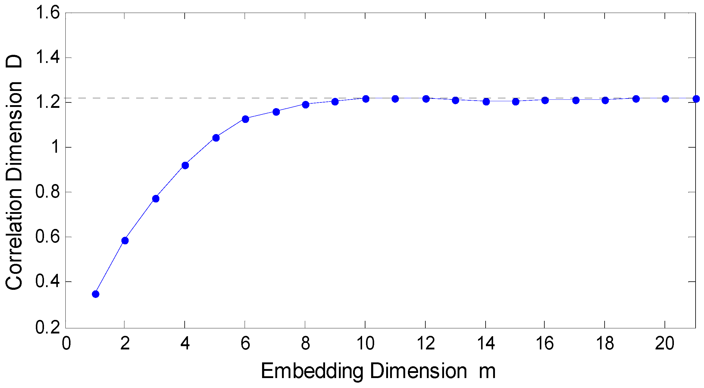
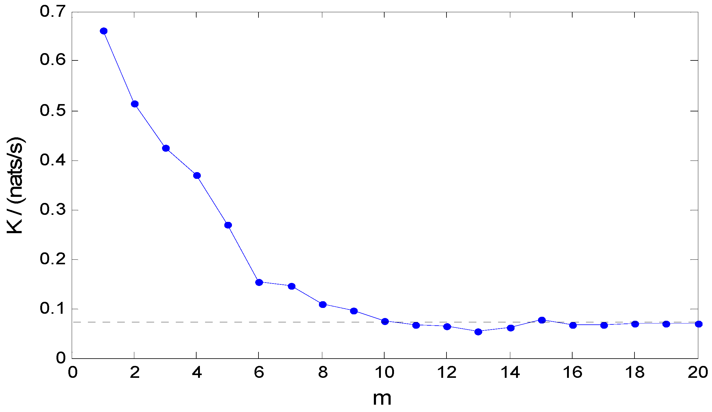
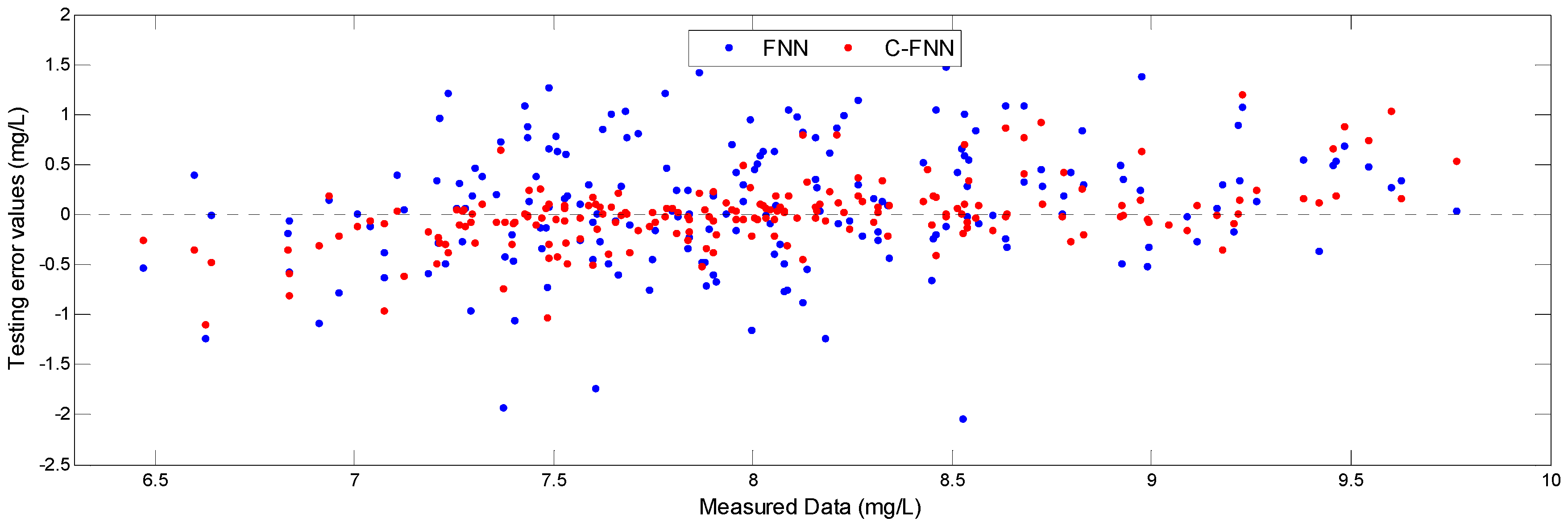
A novel soft measurement modeling method based on chaos theory and ANN for effluent BOD in WWTP is proposed in this paper. The chaotic characteristic of the WWTP has been first discovered by the fractional correlation dimension D, the positive Largest Lyapunov Exponent λ₁ and Kolmogorov entropy K of the BOD, COD, pH, SS, DO time series, which is different from the conventional research points about WWTP as a pure random and irregular system. Based on the above-mentioned chaotic characteristic, the chaos-ANN model, which combines chaos theory (i.e., PSR) with ANN, is further represented for the prediction of BOD time series.

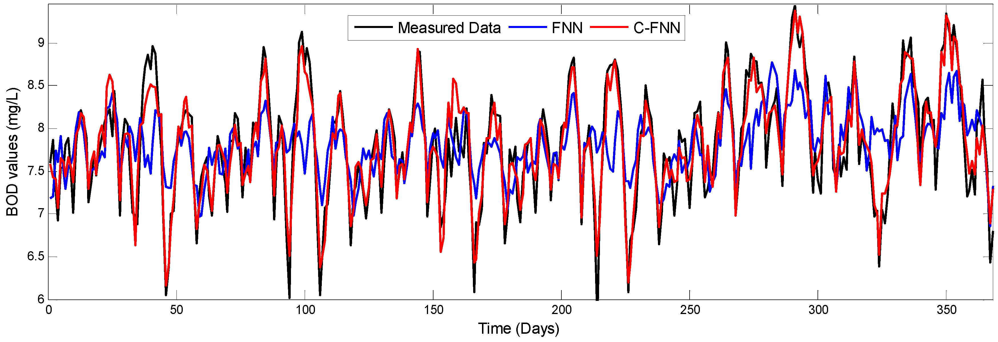
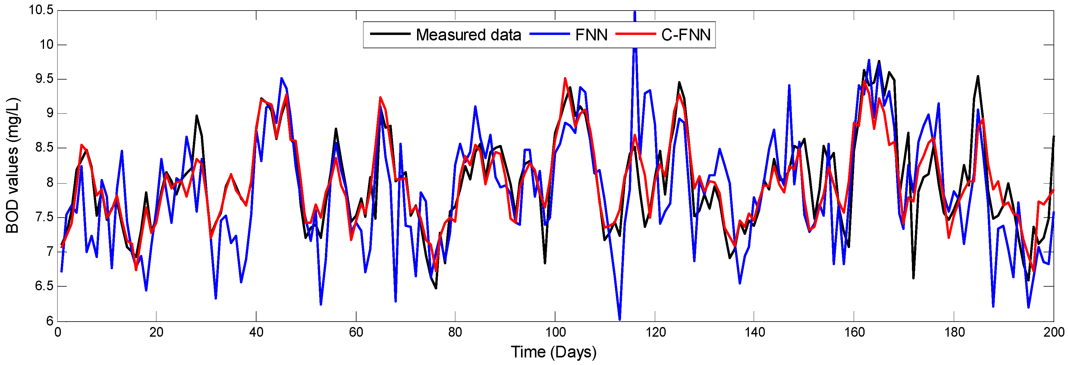
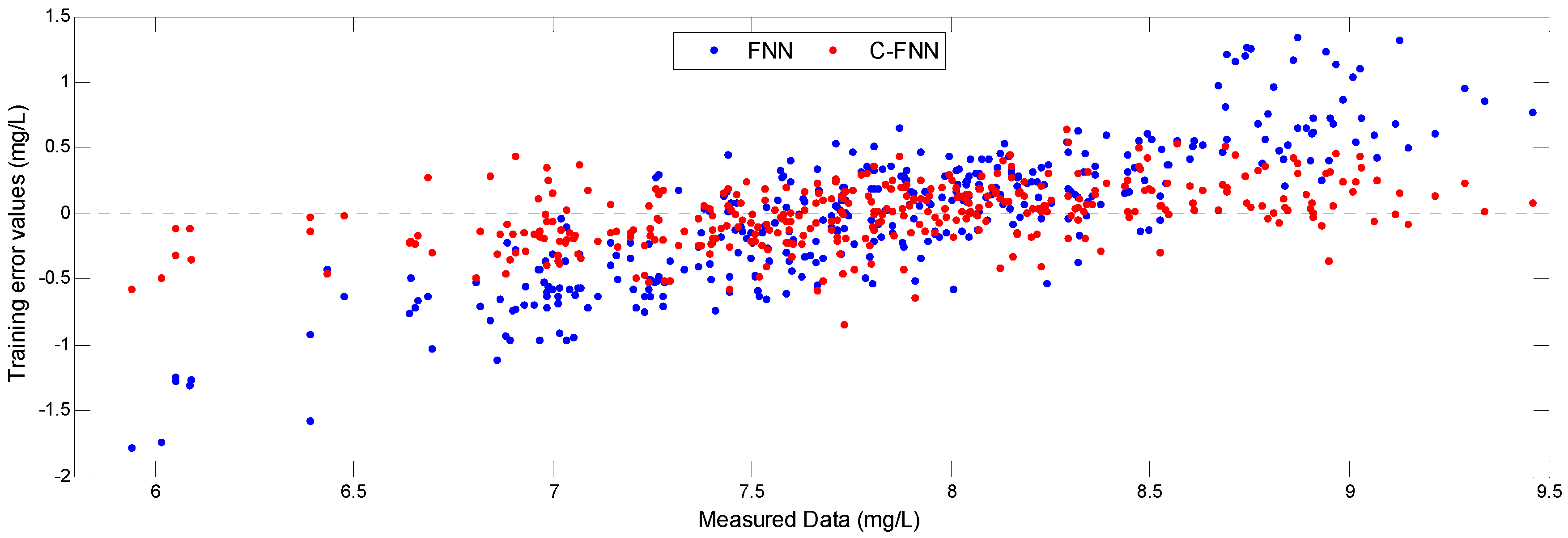
The numerical experiments demonstrated that the proposed soft measurement modeling method based on chaos theory with the suitable m and τ has higher accuracy than the corresponding modeling method not based on chaos theory. Meanwhile, de-noised data, appropriate inputs and modeling parameters can contribute to the prediction precision. If one system has been proved to be a chaotic, the chaos theory can be added into the soft measurement model to improve the accuracy of prediction. The method can be expanded to other nonlinear modeling approaches for soft measurement and other similar practical engineering applications. Beside, further work will be performed to improve its convenience and integration for better application.

References

1. Qiao, J.; Li, W.; Han, H. Soft Computing of Biochemical Oxygen Demand Using an Improved T-S Fuzzy Neural Network. Chin. J. Chem. Eng. 2014, 22, 1254–1259. [Google Scholar] [CrossRef]
2. Udeigwe, T.K.; Wang, J.J. Biochemical Oxygen Demand Relationships in Typical Agricultural Effluents. Water Air Soil Pollut. 2010, 213, 237–249. [Google Scholar] [CrossRef]
3. Jouanneau, S.; Recoules, L.; Durand, M.J.; Boukabache, A.; Picot, V.; Primault, Y. Methods for assessing biochemical oxygen demand (BOD): A review. Water Res. 2013, 49, 62–82. [Google Scholar] [CrossRef] [PubMed]
4. Han, H.; Chen, Q.; Qiao, J. Research on an online self-organizing radial basis function neural network. Neural Comput. Appl. 2010, 19, 667–676. [Google Scholar] [CrossRef] [PubMed]
5. Jin, H.; Hwang, S.J.; Shin, J.K. Using synchronous fluorescence technique as a water quality monitoring tool for an urban river. Water Air Soil Pollut. 2008, 191, 231–243. [Google Scholar]
6. Huang, M.; Ma, Y.; Wan, J.; Chen, X. A sensor-software based on a genetic algorithm-based neural fuzzy system for modeling and simulating a wastewater treatment process. Appl. Soft Comput. 2015, 27, 1–10. [Google Scholar] [CrossRef]
7. Liu, W.C.; Chung, C.E. Enhancing the predicting accuracy of the water stage using a physical-based model and an artificial neural network-genetic algorithm in a river system. Water 2014, 6, 1642–1661. [Google Scholar] [CrossRef]
8. Cheng, C.T.; Niu, W.J.; Feng, Z.K.; Shen, J.; Chau, K. Daily reservoir runoff forecasting method using artificial neural network based on quantum-behaved particle, swarm optimization. Water 2015, 7, 4232–4246. [Google Scholar] [CrossRef]
9. Han, H.G.; Li, Y.; Guo, Y.N.; Qiao, J.F. A soft computing method to predict sludge volume index based on a recurrent self-organizing neural network. Appl. Soft Comput. 2016, 38, 477–486. [Google Scholar] [CrossRef]
10. Lee, B.H.; Scholz, M. A comparative study: Prediction of constructed treatment wetland performance with k-nearest neighbors and neural networks. Water Air Soil Pollut. 2006, 174, 279–301. [Google Scholar] [CrossRef]
11. Wang, W.C.; Li, K.; Chen, Z.X.; Niu, Q.Z. Soft Measurement technique of sewage treatment parameters based on wavelet neural networks. Appl. Mech. Mater. 2014, 556–562, 3168–3171. [Google Scholar] [CrossRef]
12. Wan, J.; Huang, M.; Ma, Y.; Guo, W.; Wang, Y.; Zhang, H.; Sun, X. Prediction of effluent quality of a paper mill wastewater treatment using an adaptive network-based fuzzy inference system. Appl. Soft Comput. 2011, 11, 3238–3246. [Google Scholar] [CrossRef]
13. Heddam, S.; Lamda, H.; Filali, S. Predicting effluent biochemical oxygen demand in a wastewater treatment plant using generalized regression neural network based approach: A comparative study. Environ. Process. 2016, 3, 153–165. [Google Scholar] [CrossRef]
14. Vyas, M.; Modhera, B.; Vyas, V.; Sharma, A.K. Performance forecasting of common effluent treatment plant parameter by artificial neural network. J. Eng. Appl. Sci. 2011, 6, 38–42. [Google Scholar]
15. Trapani, D.D.; Mannina, G.; Torregrossa, M.; Viviani, G. Quantification of kinetic parameters for heterotrophic bacteria via respirometry in a hybrid reactor. Water Sci. Technol. 2010, 61, 1757–1766. [Google Scholar] [CrossRef] [PubMed]
16. Hussain, A.; Al-Rawajfeh, A.E.; Alsaraierh, H. Membrane bio reactors (MBR) in waste water treatment: A review of the recent patents. Recent Pat. Biotechnol. 2010, 4, 65–80. [Google Scholar] [CrossRef] [PubMed]
17. Liu, Y.; Lei, S.; Sun, C.; Zhou, Q.; Ren, H. A multivariate forecasting method for short-term load using chaotic features and RBF neural network. Eur. Trans. Electr. Power 2011, 21, 1376–1391. [Google Scholar] [CrossRef]
18. Fan, X.; Li, S.; Tian, L. Chaotic characteristic identification for carbon price and an multi-layer perceptron network prediction model. Expert Syst. Appl. 2015, 42, 3945–3952. [Google Scholar] [CrossRef]
19. Zhang, Z.; Wang, T.; Liu, X. Melt index prediction by aggregated RBF neural networks trained with chaotic theory. Neurocomputing 2014, 131, 368–376. [Google Scholar] [CrossRef]
20. Zhang, L.; Tian, F.; Liu, S.; Dang, L.; Peng, X.; Yin, X. Chaotic time series prediction of E-nose sensor drift in embedded phase space. Sens. Actuator B Chem. 2013, 182, 71–79. [Google Scholar] [CrossRef]
21. Liang, Q.Z.; Guo, X.M.; Zhang, W.Y.; Dai, W.D.; Zhu, X.H. Identification of heart sounds with arrhythmia based on recurrence quantification analysis and Kolmogorov entropy. J. Med. Biol. Eng. 2015, 35, 209–217. [Google Scholar] [CrossRef]
22. Yang, L.; Zhang, J.; Wu, X.; Zhang, Y.; Li, J. A chaotic time series prediction model for speech signal encoding based on genetic programming. Appl. Soft Comput. 2015, 38, 754–761. [Google Scholar] [CrossRef]
23. Takens, F. Detecting strange attractors in turbulence. In Dynamical Systems and Turbulence, Warwick 1981; Springer: Berlin/Heidelberg, Germany, 1981; pp. 366–381. [Google Scholar]
24. Chandra, R.; Zhang, M. Cooperative coevolution of Elman recurrent neural networks for chaotic time series prediction. Neurocomputing 2012, 86, 116–123. [Google Scholar] [CrossRef]
25. Li, Z.M.; Cui, L.G.; Xu, S.W.; Weng, L.Y.; Dong, X.X.; Li, G.Q.; Yu, H.P. Prediction model of weekly retail price for eggs based on chaotic neural network. J. Integr. Agric. 2013, 12, 2292–2299. [Google Scholar] [CrossRef]
26. Hanias, M.P.; Karras, D.A. On efficient multistep non-linear time series prediction in chaotic diode resonator circuits by optimizing the combination of non-linear time series analysis and neural networks. Eng. Appl. Artif. Intell. 2009, 22, 32–39. [Google Scholar] [CrossRef]
27. Han, M.; Wang, Y. Analysis and modeling of multivariate chaotic time series based on neural network. Expert Syst. Appl. 2009, 36, 1280–1290. [Google Scholar]
28. Su, L.Y. Prediction of multivariate chaotic time series with local polynomial fitting. Comput. Math. Appl. 2010, 59, 737–744. [Google Scholar] [CrossRef]
29. Chen, D.; Han, W. Prediction of multivariate chaotic time series via radial basis function neural network. Complexity 2013, 18, 55–66. [Google Scholar] [CrossRef]
30. Kim, H.; Eykholt, R.; Salas, J.D. Nonlinear dynamics, delay times, and embedding windows. Phys. D Nonlinear Phenom. 1999, 127, 48–60. [Google Scholar] [CrossRef]
31. Hacine-Gharbi, A.; Ravier, P.; Harba, R.; Mohamadi, T. Low bias histogram-based estimation of mutual information for feature selection. Pattern Recognit. Lett. 2012, 33, 1302–1308. [Google Scholar] [CrossRef]
32. Grassberger, P.; Procaccia, I. Measuring the strangeness of strange attractors. Phys. D Nonlinear Phenom. 1983, 9, 189–208. [Google Scholar] [CrossRef]
33. Grassberger, P.; Procaccia, I. Characterization of strange attractors. Phys. Rev. Lett. 1983, 50, 346–349. [Google Scholar] [CrossRef]
34. Cao, L. Practical method for determining the minimum embedding dimension of a scalar time series. Phys. D Nonlinear Phenom. 1997, 110, 43–50. [Google Scholar] [CrossRef]
35. Chai, S.H.; Lim, J. Forecasting business cycle with chaotic time series based on neural network with weighted fuzzy membership functions. Chaos Soliton Fractal 2016, 90, 118–126. [Google Scholar] [CrossRef]
36. Wolf, A.; Swift, J.B.; Swinney, H.L.; Vastano, J.A. Determining Lyapunov exponents from a time series. Phys. D Nonlinear Phenom. 1985, 16, 285–317. [Google Scholar] [CrossRef]
37. Grassberger, P.; Procaccia, I. Estimation of the Kolmogorov entropy from a chaotic signal. Phys. Rev. A 1983, 28, 2591–2593. [Google Scholar] [CrossRef]
38. Han, H.G.; Qiao, J.F. Prediction of activated sludge bulking based on a self-organizing RBF neural network. J. Process Control 2012, 22, 1103–1112. [Google Scholar] [CrossRef]
39. Han, H.G.; Qian, H.H.; Qiao, J.F. Nonlinear multi-objective model-predictive control scheme for waste water treatment process. J. Process Control 2014, 24, 47–59. [Google Scholar] [CrossRef]
Figure 1. Activated sludge process in a wastewater treatment plant (WWTP).
Water 08 00581 g001
Figure 2. The structure of the prediction model based on chaos theory for BOD with PCA-ANN.
Water 08 00581 g002
Figure 3. The original measured data used for effluent BOD modeling.
Water 08 00581 g003
Figure 4. Mutual information I(τ) of different τ for BOD dataset.
Water 08 00581 g004
Figure 5. The curves of lnrlnC(r) for BOD dataset.
Water 08 00581 g005
Figure 6. The curves of D over m for the BOD dataset.
Water 08 00581 g006
Figure 7. Two-dimension phase space portrait of BOD dataset.
Water 08 00581 g007
Figure 8. The curves of m-K for BOD dataset.
Water 08 00581 g008
Figure 9. The variance explained by the principal components.
Water 08 00581 g009
Figure 10. The training output of the FNN, C-FNN for BOD.
Water 08 00581 g010
Figure 11. The testing output of the FNN, C-FNN for BOD.
Water 08 00581 g011
Figure 12. The training error of the FNN, C-FNN for BOD.
Water 08 00581 g012
Figure 13. The testing error of the FNN, C-FNN for BOD.
Water 08 00581 g013