Sinuosity-Driven Water Pressure Distribution on Slope of Slightly-Curved Riparian Zone: Analytical Solution Based on Small-disturbance Theory and Comparison to Experiments

Abstract

A curved riparian zone can create highly complex flow patterns that have a great effect on erosion, pollutant transport, surface water-groundwater exchange and habitat qualities. The small-disturbance theory has been applied to derive the analytical solutions of pressure distributions along a sinusoidal riverbank. Experiments have also been performed to test the hydrodynamic and geomorphic effects on pressure distribution and to verify the applicability of the derived expressions. The derived expressions were simple, accurate and agreed remarkably well with experimental results for the riparian banks with a low degree of curvature. On the contrary, when a riparian bank had a high degree of curvature, these expressions applying the approach of small-disturbance, could not effectively estimate the pressure distributions for a complex bank boundary or complex flow conditions. Moreover, sensitive analysis has indicated that the disturbed pressures along the riparian banks increased with increasing Froude number Fr, as well as the ratio of bank amplitude to wavelength a/λ. However, a/λ has been found to have more significant influence on pressure variation in subcritical flow.

1. Introduction

A river’s topographic features interact with water to create highly complex flow patterns [1]. For instance, aided by an exaggerated superelevation near the bend apex of a curved riparian zone, a turbidity current may split [2,3,4,5,6], and hyporheic exchange occurs over a wide range of topography scales of meandering riparian zones [7,8,9,10]. It is evident that these flow patterns are much more complicated than those in straight rivers [11,12,13,14]. These complicated flow patterns due to a curved riparian zone have a great effect on erosion, sediment, pollutant transport, and surface-ground water exchange in rivers [11,15] and play a significant role in determining qualities of habitat and environment. Because of these, curved riparian zones have been the focus on the preservation of river ecology, the design of river restoration works and have even become central to river restoration plans [14,16]. In the past three decades, many studies on various aspects of curved channel flow have been conducted, leading to considerable advances in the understanding of flow mechanism in curved rivers. Many mathematical studies have been carried out to attempt to gain a clear understanding of the flow characteristics in curved open channels [12]. Hicks et al. (1990) investigated the flow in a smooth half trapezoidal channel bend, with particular emphasis on the outside bank details [11,15]. The vertically averaged and moment equation model developed by Ghamry (1999), with presumed linear or quadratic distributions of horizontal velocity components and quadratic vertical velocity and pressure distributions, has been used [17]. Generally, these studies have concentrated on understanding the flow and erosion patterns away from the banks of wide, relatively gently curving shallow channels. It was found that boundary stresses on the outside curved bank were significantly higher than in a straight channel and did not diminish until very close to the top of the bank [15]. Buffington and Tonina (2009) summarized the relative importance of different mechanisms for generating hyporheic processes in eight types of mountain rivers [7]. They considered pressure gradient on the face of a riparian zone as one of the most important driving forces for stream-subsurface exchange. The mechanisms contributing to exchanges are not yet fully understood [18,19]. This is because there is insufficient knowledge regarding the process of near-bank pressure variations induced by bank morphology [18,19]. Despite substantial research on various aspects of the velocity distribution in curved meandering rivers, no systematic effort has been made to analyze the variation of the pressure profile along a meander path [14]. Thus, the proper simulation and prediction of the near-bank pressure field will facilitate the further study on the lateral hyporheic exchange, contaminant transport, and the circulation of ecologically relevant substances between rivers and riparian zones [20].

Researchers have discovered that certain small perturbations to a laminar flow can cause an extremely large transient energy growth in a linearized system [21]. It has been suggested that when the transient growth becomes “sufficiently large”, the flow is “mixed” by the nonlinearity, producing turbulence [21,22]. This approach can be roughly summarized by saying that flow systems are extremely sensitive to small perturbations in the initial flow [21,22,23,24]. The advantage of a small disturbance method lies in the fast direct calculation of flow amplitudes compared to their extraction after a time-costly unsteady flow calculation [25], which has been widely used in aerodynamics to solve problems of hypersonic, subsonic or transonic flow over a thin aerofoil and has been verified by experiments [22]. Because the sinuous channel flow is a type of superposition consisting of uniform flow and disturbed flow induced by a sinuous riparian apex, the small-disturbance theory can be extended to solve the problem of flow at the boundary of a curved bank as long as the disturbance is small enough. For instance, the variety of parameters in surface-groundwater interaction investigations, e.g., water pressure, demands a time-efficient and accurate method for calculating the unsteady water pressures distribution. To work towards this goal, small-disturbance Saint-Venant equations based on full Saint-Venant equations were developed. Therefore, the purposes of the study are (1) to derive small-disturbance Saint-Venant equations from relatively reduced-order full Saint-Venant models to yield the analytical solutions of water pressure on the surface of a sinuous riparian zone, (2) to investigate the accuracy of the analytical solution by comparing with experimental data to emphasize that extremely small disturbances can cause very large changes in solutions of nonlinear partial differential equations, and (3) to demonstrate how the main control morphology parameters act on water pressure distribution and to identify which one parameter is the most sensitive through sensitivity analysis. It is anticipated that the results of such a study will provide a valuable method for better linking the hydraulic characteristics of a curved river to the spatial and temporal hydrologic attributes of surface water-groundwater interactions, as well as to the ecological attributes of streams.

2. Methods

2.1. Fundamental Equations

A natural river is conceptualized as a generic meandering river, which is characterized by a shallow-water river in which the vertical pressure distribution is approximately hydrostatic and the vertical acceleration is so small that it can be ignored. Two-dimensional modelling of open-channel flows usually uses the depth-averaged shallow-water equations (SWEs), in which the vertical acceleration of the fluid is ignored [26]. The SWEs, without considering wind resistance and the Coriolis force [27], are expressed as follows.

Continuity Equation:

$$\frac{\partial (hu)}{\partial x}+\frac{\partial (hv)}{\partial y}=0$$

(1)

Momentum Equations:

$$u\frac{\partial u}{\partial x}+v\frac{\partial u}{\partial y}=-g\frac{\partial \mathsf{\zeta }}{\partial x}-\frac{g{n}^{2}u\sqrt{u^2+v^2}}{h^{4/3}}+\frac{{\mathsf{\mu }}_{eff}}{\mathsf{\rho }}[\frac{{\partial }^2(hu)}{\partial x^2}+\frac{{\partial }^2(hu)}{\partial y^2}]$$

(2)

$$u\frac{\partial v}{\partial x}+v\frac{\partial v}{\partial y}=-g\frac{\partial \mathsf{\zeta }}{\partial y}-\frac{g{n}^{2}v\sqrt{u^2+v^2}}{h^{4/3}}+\frac{{\mathsf{\mu }}_{eff}}{\rho }[\frac{{\partial }^2(hv)}{\partial x^2}+\frac{{\partial }^2(hv)}{\partial y^2}]$$

(3)

where x, y are the coordinates in the downstream and cross-stream directions, respectively; u, v are depth-averaged flow velocities in the x and y directions, respectively; g is the acceleration of gravity; h is water depth; ζ is water surface elevation; n is Manning’s roughness coefficient; μ_eff is viscosity, which consists of the molecule viscosity, μ, and the turbulent eddy viscosity, μ_t. The second terms on the right-hand side of Equation (2) and Equation (3) are the bed resistance terms, induced by viscosity.

In a natural river, the flow can be considered as potential flow because viscosity has significant influence on the flow regime only within a confined thin boundary layer, while viscous effects have little impact outside of the boundary layer. Therefore, viscous effects are ignored and water pressure distribution on the surface can be approximately analyzed according to the potential flow regime if the boundary layer does not separate from the body surface. Assuming a flat river bedform and the flow is inviscouse and steady, Equations (1), (2) and (3) can be simplified to Equations (4), (5) and (6), respectively.

Continuity Equation:

$$\frac{\partial (hu)}{\partial x}+\frac{\partial (hv)}{\partial y}=0$$

(4)

Momentum Equations:

$$u\frac{\partial u}{\partial x}+v\frac{\partial u}{\partial y}=-g\frac{\partial h}{\partial x}$$

(5)

$$u\frac{\partial v}{\partial x}+v\frac{\partial v}{\partial y}=-g\frac{\partial h}{\partial y}$$

(6)

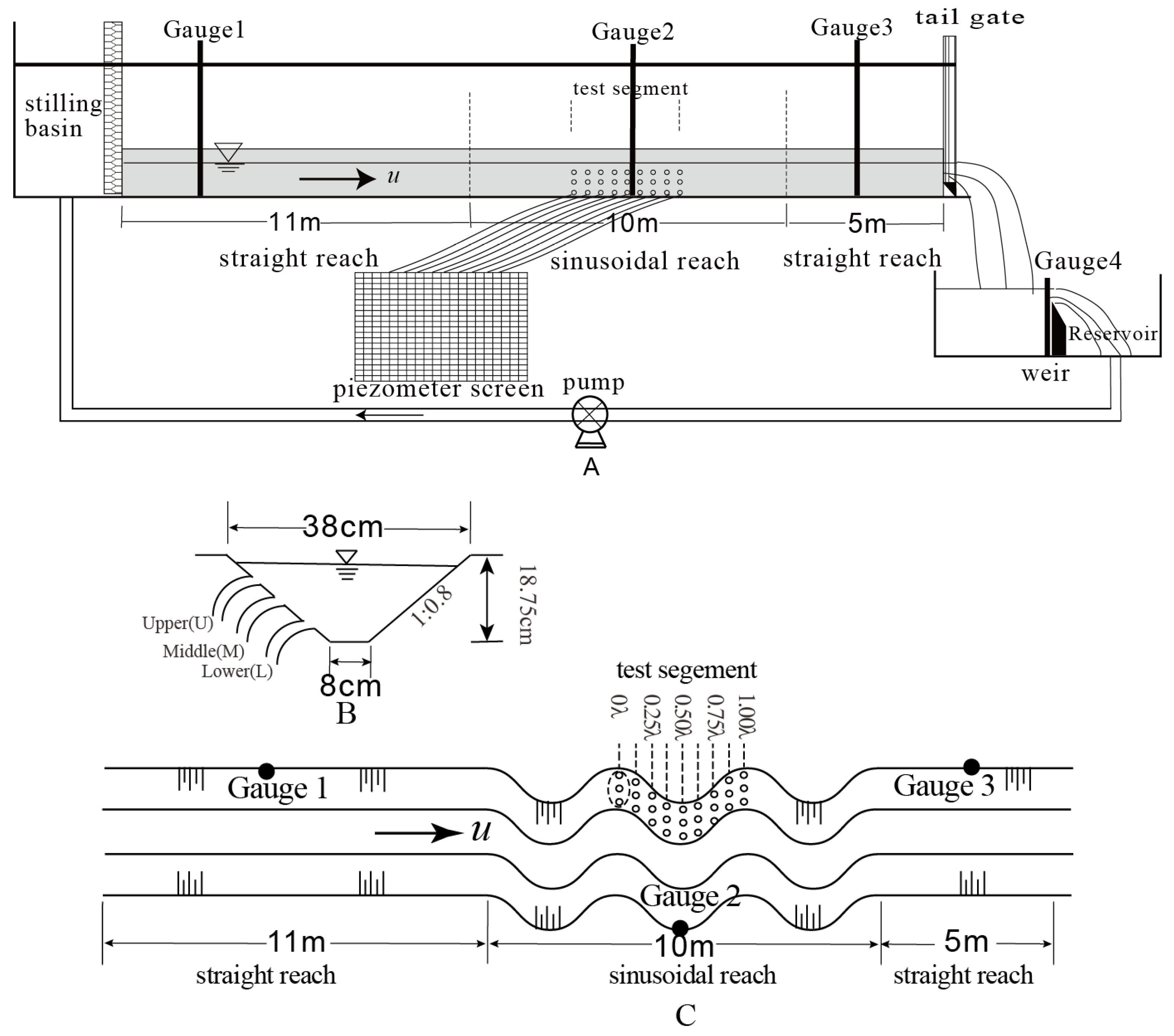
2.2. Experimental Setups

Experiments were conducted in a 26 m long, 0.5 m wide and 0.7 m deep glass-walled flume [28,29] whose slope was fixed at 0.07692% (Figure 1A). A sinuous channel module made from polyvinyl chloride plastic, of which the bed was 8 cm wide and the top was 38 cm wide and the side slope coefficient was 1:0.8 and the height of side slope is 18.75 cm and the right and left banks were symmetrical, was set in the flume to form the geomorphology of a wide-shallow sinuous river (Figure 1B). Meanwhile, the face of module was very smooth to keep flow as inviscouse as possible. The sinuous river consisted of three reaches: upstream straight reach (11 m length), middle sinusoidal reach (10 m length) and downstream straight reach (5 m length) (Figure 1C). In the middle reach, the right and left bank-lines were curved as a sinusoidal wave in the stream-wise direction, whose amplitude, a, took values of 4 cm or 8 cm and wave length, λ, took values of 50 cm, 100 cm or 200 cm (

Table 1. Summary of Flow Conditions in Experiment.

Runs	a/cm	λ/cm	Q/(l·s−1)	h0/cm	a/λ	Fr
Run1	8	200	5.90	10.77	0.04	0.40
Run2	8	200	7.90	10.78	0.04	0.53
Run3	8	200	9.17	10.78	0.04	0.65
Run4	4	100	12.02	13.29	0.04	0.53
Run5	8	100	12.00	13.30	0.08	0.53
Run6	8	50	3.42	13.30	0.16	0.15

Notes: a and λ are the amplitude and wavelength of a sinusoidal bank, respectively; Fr is the Froude number of flow.

) [29]. A central full wave segment of right bank with a specific bank form wavelength(λ) in the middle reach was selected as our test segment. Within the test segment, nine cross sections, located at 0λ, 0.125λ, 0.25λ, 0.375λ, 0.5λ, 0.625λ, 0.75λ, 0.875λ, and 1λ section, respectively, were set as pressure measured sections with 0.125λ intervals in the right bank. With a specific wavelength(λ), the 0λ section was located at 16–0.5λ from upstream. To investigate the pressures in different layers on the slope face of right bank, three holes on the slope face of each cross section of right bank, 2 cm, 5 cm and 8 cm away from slope toe, respectively, were drilled and connected to the water head screen with 27 piezometers, through which water heads on upper, middle and lower layers of bank slope were recorded (Figure 1). Additionally, two straight reaches were used as transitional segments to smooth flow into or out of the middle reach. Water was pumped into a stilling basin and flowed into the flume. The flow surface profile in the river was controlled by the downstream tailgate, which was installed at the end of the flume and was adjustable by means of a gear system, allowing its opening size to be set with a high degree of accuracy. The two transition reaches and tail gate prevented the occurrence of large-scale disturbances of the inlet and outlet and allowed for the development of a quasi-constant water depth flow from upstream to downstream to keep flow as steady as possible. The outlet and the inlet structures of the flume were connected to a hydraulic circuit, allowing a continuous recirculation of stable discharges. The experimental cases and conditions are summarized in Table 1.

3. Results

3.1. Theoretical Equations and Analytical Solutions

3.1.1. Theoretical Equations

In this section the transformation of the conservative full Saint-Venant equations for Cartesian coordinates in small disturbance formulations is presented. According to small-disturbance theory, the flow quantities indicated by Ψ are split into two parts: a steady quantity and an unsteady periodic quantity $\Psi ={\Psi }_{\infty }+\tilde{\Psi }$, where Ψ_∞ is the steady quantity; $\tilde{\Psi }$ is the unsteady periodic quantity. Applying this approach, the equations can be split into a steady and an unsteady problem. The unsteady part leads to an eigenvalue problem, assuming simple harmonic vibration.

It is assumed that a uniform flow enters into a sinusoidal river with width b, as in Figure 2. The incoming uniform flow velocity and depth are $u_{\infty }$ and $h_{\infty }$, respectively.

Due to the sinusoidal form of the bank, flow velocities (in the x and y directions) and water depth are disturbed. When the bank is so low curved that the flow does not separate from the bank, variation of the flow velocities and depth is very small and the sinusoidal bank form can be considered as a small disturbance. Therefore, the kinematic variables of u, v and h can be re-formulated as the sum of uniform and disturbance components:

$$u=u_{\infty }+\tilde{u}$$

(7)

$$v=\tilde{v}$$

$$h=h_{\infty }+\tilde{h}$$

where $u_{\infty }$ and $h_{\infty }$ are the velocity and depth of incoming uniform flow, respectively; $\tilde{u}$ and $\tilde{v}$ are the disturbed velocities in the x and y directions, respectively; $\tilde{h}$ is the disturbed flow depth. $\frac{\partial \tilde{u}}{\partial x}$, $\frac{\partial \tilde{u}}{\partial y}$, $\frac{\partial \tilde{v}}{\partial x}$, $\frac{\partial \tilde{v}}{\partial y}$, $\frac{\partial \tilde{h}}{\partial x}$ and $\frac{\partial \tilde{h}}{\partial y}$ are the first-order small variables and $|\tilde{u}/u_{\infty }|\ll 1$, $|\tilde{v}/u_{\infty }|\ll 1$ and $|\tilde{h}/h_{\infty }|\ll 1$.

We insert Equation (7) into Equations (4)–(6) and the second-order terms are ignored because they are too small. Then, Equations (4)–(6) can be reformulated as Equations (8)–(10), which are referred to as small-disturbance equations.

$$h_{\infty }\frac{\partial \tilde{u}}{\partial x}+u_{\infty }\frac{\partial \tilde{h}}{\partial x}+h_{\infty }\frac{\partial \tilde{v}}{\partial y}=0$$

(8)

$$h_{\infty }\frac{\partial \tilde{u}}{\partial x}=-\mathrm{g}\frac{\partial \tilde{h}}{\partial x}$$

(9)

$$u_{\infty }\frac{\partial \tilde{v}}{\partial x}=-\mathrm{g}\frac{\partial \tilde{h}}{\partial y}$$

(10)

Combining Equations (8) and (9) with Equation (10), the small-disturbance equations are compounded as Equation (11).

$$(1-F{r}^2)\frac{{\partial }^2\tilde{h}}{\partial x^2}+\frac{{\partial }^2\tilde{h}}{\partial y^2}=0$$

(11)

where $Fr=u_{\infty }/\sqrt{\mathrm{g}{h}_{\infty }}$ is the Froude number of incoming uniform flow.

Because the flow regime in most natural rivers is subcritical flow (Fr < 1) and $\sqrt{1-F{r}^2}$ is defined as a new variable of $w$, the simplified form of Equation (11) is expressed as Equation (12), which is an elliptical equation.

$$w^2\frac{{\partial }^2\tilde{h}}{\partial x^2}+\frac{{\partial }^2\tilde{h}}{\partial y^2}=0$$

(12)

3.1.2. Problem Statement

Supposing that the disturbed depth ${\tilde{h}}_0$ is at the reference original point (0, 0), the boundary condition at position (0, 0) can be defined as:

$${\tilde{h}|}_{\begin{array}{c}x=0\\ y=0\end{array}}={\tilde{h}}_0$$

(13)

We set the normal vector of the wall and flow velocity vector as $\stackrel{\rightharpoonup }{n}$ and $\stackrel{\rightharpoonup }{V}$, respectively. Then, the wall boundary condition can be expressed as:

$$\stackrel{\rightharpoonup }{V}·\stackrel{\rightharpoonup }{n}=0$$

(14)

Given the wall function y = f(x), its normal vector $\stackrel{\rightharpoonup }{n}$ can be defined as:

$$\stackrel{\rightharpoonup }{n}=(-\frac{\partial f}{\partial x},1)$$

(15)

Substituting Equation (15) into Equation (14),

$$\stackrel{\rightharpoonup }{V}\cdot \stackrel{\rightharpoonup }{n}=(u,v)\cdot (-\frac{\partial f}{\partial x},1)=-u\frac{\partial f}{\partial x}+v=0$$

(16)

Substituting Equation (7) into Equation (16) and ignoring the second-order and higher order terms of small variations, we get

$$-u_{\infty }\frac{\partial f}{\partial x}+\tilde{v}=0$$

(17)

Substituting Equation (17) into Equation (10), the wall boundary condition is defined as:

$$\frac{\partial \tilde{h}}{\partial y}=-\frac{u_{\infty }}{g}\frac{\partial \tilde{v}}{\partial x}=-\frac{u_{\infty }^2}{g}\frac{{\partial }^{2}f}{\partial x^2}$$

(18)

If we suppose that the right bank wall function is $y_1=f_1\left(x\right)=a\sin \frac{2\mathsf{\pi }}{\mathsf{\lambda }}x$ and the left wall function is $y_2=f_2\left(x\right)=a\sin \frac{2\mathsf{\pi }}{\mathsf{\lambda }}x+b$, where a and λ are the amplitude and the wavelength of the sinusoidal bank, respectively, and b is the width of the river, and assume that a/λ is much less than 1 ($\mathrm{a}/\mathsf{\lambda }\ll 1$), the wall boundary conditions could be approximately expressed as:

Right wall boundary condition:

$${\frac{\partial \tilde{h}}{\partial y}|}_{y=0}=-\frac{u_{\infty }^2}{g}\frac{{\partial }^2{f}_1}{\partial x^2}=\frac{u_{\infty }^{2}a}{g}{(\frac{2\mathsf{\pi }}{\mathsf{\lambda }})}^2\cdot \sin \frac{2\mathsf{\pi }}{\mathsf{\lambda }}x$$

(19)

Left wall boundary condition

$${\frac{\partial \tilde{h}}{\partial y}|}_{y=b}=-\frac{u_{\infty }^2}{g}\frac{{\partial }^2{f}_2}{\partial x^2}=\frac{u_{\infty }^{2}a}{g}{(\frac{2\mathsf{\pi }}{\mathsf{\lambda }})}^2\cdot \sin \frac{2\mathsf{\pi }}{\mathsf{\lambda }}x$$

(20)

In summary, when we combine Equation (12) with boundary condition Equation (20), the problem of water pressure distribution on the bank face of a sinusoidal river can be described as a boundary-value problem.

$$\{\begin{array}{c}{w}^2\frac{{\partial }^2\tilde{h}}{\partial x^2}+\frac{{\partial }^2\tilde{h}}{\partial y^2}=0 x>0 \\ \tilde{\mathrm{h}}{|}_{\mathrm{x}=0}=0 \\ \frac{\partial \tilde{\mathrm{h}}}{\partial \mathrm{y}}{|}_{\mathrm{y}=0}=\frac{{\mathrm{u}}_0\mathrm{a}}{\mathrm{g}}{\left(\frac{2\mathsf{\pi }}{\mathsf{\lambda }}\right)}^2·\sin \frac{2\mathsf{\pi }}{\mathsf{\lambda }}x \\ \frac{\partial \tilde{\mathrm{h}}}{\partial \mathrm{y}}{|}_{\mathrm{y}=\mathrm{b}}=\frac{{\mathrm{u}}_0\mathrm{a}}{\mathrm{g}}{\left(\frac{2\mathsf{\pi }}{\mathsf{\lambda }}\right)}^2·\sin \frac{2\mathsf{\pi }}{\mathsf{\lambda }}x \end{array}$$

(21)

3.1.3. Analytical Solutions

Because Equation (21) is a boundary-value problem, it can be solved by using the separating variable method such that the analytical solution of water pressure can be obtained as Equation (22).

$$\tilde{h}(x,y)={\tilde{h}}_0+\frac{2a{u}_{\infty }^2}{bg}{(\frac{2\mathsf{\pi }}{\mathsf{\lambda }})}^2\sin \frac{2\mathsf{\pi }}{\mathsf{\lambda }}x\cdot {\displaystyle \sum _{n=1}^{\infty }[{(-1)}^n}-1]\frac{1}{{(\frac{2\mathsf{\pi }w}{\mathsf{\lambda }})}^2+{(\frac{n\mathsf{\pi }}{b})}^2}\cos \frac{n\mathsf{\pi }}{b}y$$

(22)

To make Equation (22) more explicit, we construct a function as Equation (23),

Constructed Function:

$$\exp (2\mathsf{\pi }wy/\mathsf{\lambda })-\exp (2\mathsf{\pi }wb/\mathsf{\lambda })\cdot \exp (-2\mathsf{\pi }wy/\mathsf{\lambda })$$

(23)

Then, Fourier-cosine series expansion of Equation (23) on interval [0, b] is gained as Equation (24)

$$\begin{gathered} \exp (2\mathsf{\pi }wy/\mathsf{\lambda })-\exp (2\mathsf{\pi }wb/\mathsf{\lambda })\cdot \exp (-2\mathsf{\pi }wy/\mathsf{\lambda }) \\ =[\exp (2\mathsf{\pi }wb/\mathsf{\lambda })+1]\cdot \frac{4\mathsf{\pi }w}{b\mathsf{\lambda }}\cdot {\displaystyle \sum _{n=1}^{\infty }[{(-1)}^n}-1]\frac{1}{{(\frac{2\mathsf{\pi }w}{\mathsf{\lambda }})}^2+{(\frac{n\mathsf{\pi }}{b})}^2}\cos \frac{n\mathsf{\pi }}{b}y \end{gathered}$$

(24)

Comparing Equation (22) with (24), $\tilde{h}(x,y)$ can be explicitly expressed as:

$$\tilde{h}(x,y)={\tilde{h}}_0+\frac{2\mathsf{\pi }a{u}_{\infty }^2}{\mathsf{\lambda }gw}\cdot \frac{\exp (2\mathsf{\pi }wy/\mathsf{\lambda })-\exp (2\mathsf{\pi }wb/\mathsf{\lambda })\cdot \exp (-2\mathsf{\pi }wy/\mathsf{\lambda })}{\exp (2\mathsf{\pi }wb/\mathsf{\lambda })+1}\sin \frac{2\mathsf{\pi }}{\mathsf{\lambda }}x$$

(25)

Substituting y = 0 and y = b into Equation (25), respectively, the explicit expressions of the disturbed pressure heads on the right bank and left bank are obtained as Equations (26) and (27), respectively.

Right bank:

$${\tilde{h}|}_{y=0}={\tilde{h}}_0-\frac{2\pi a{u}_{\infty }^2}{\lambda gw}\cdot \frac{\exp (2\pi wb/\lambda )-1}{\exp (2\pi wb/\lambda )+1}\cdot \sin \frac{2\pi }{\lambda }x$$

(26)

Left bank:

$${\tilde{h}|}_{y=b}={\tilde{h}}_0+\frac{2\mathsf{\pi }a{u}_{\infty }^2}{\mathsf{\lambda }gw}\cdot \frac{\exp (2\mathsf{\pi }wb/\mathsf{\lambda })-1}{\exp (2\mathsf{\pi }wb/\mathsf{\lambda })+1}\cdot \sin \frac{2\mathsf{\pi }}{\mathsf{\lambda }}x$$

(27)

The two formulas are the necessary disturbed parts of water pressure on the right and left banks. With respect to dimensionless treatment, both sides of Equations (26) and (27) are subtracted by ${\tilde{h}}_0$ and divided by $u_{\infty }^2/2\mathrm{g}$ and then dimensionless expressions of water pressure ${\tilde{h}}_{pi}^{*}$ on the right bank and left bank are obtained.

Right bank:

$${\tilde{h}}_{pi}^{*}=\frac{{\tilde{h}|}_{y=0}-{\tilde{h}}_0}{u_{\infty }^2/2g}=-\frac{4\mathsf{\pi }a}{\mathsf{\lambda }w}\cdot \frac{\exp (2\mathsf{\pi }wb/\mathsf{\lambda })-1}{\exp (2\mathsf{\pi }wb/\mathsf{\lambda })+1}\cdot \sin \frac{2\mathsf{\pi }}{\mathsf{\lambda }}x$$

(28)

Left bank:

$${\tilde{h}}_{pi}^{*}=\frac{{\tilde{h}|}_{y=0}-{\tilde{h}}_0}{u_{\infty }^2/2g}=\frac{4\mathsf{\pi }a}{\mathsf{\lambda }w}\cdot \frac{\exp (2\mathsf{\pi }wb/\mathsf{\lambda })-1}{\exp (2\mathsf{\pi }wb/\mathsf{\lambda })+1}\cdot \sin \frac{2\mathsf{\pi }}{\mathsf{\lambda }}x$$

(29)

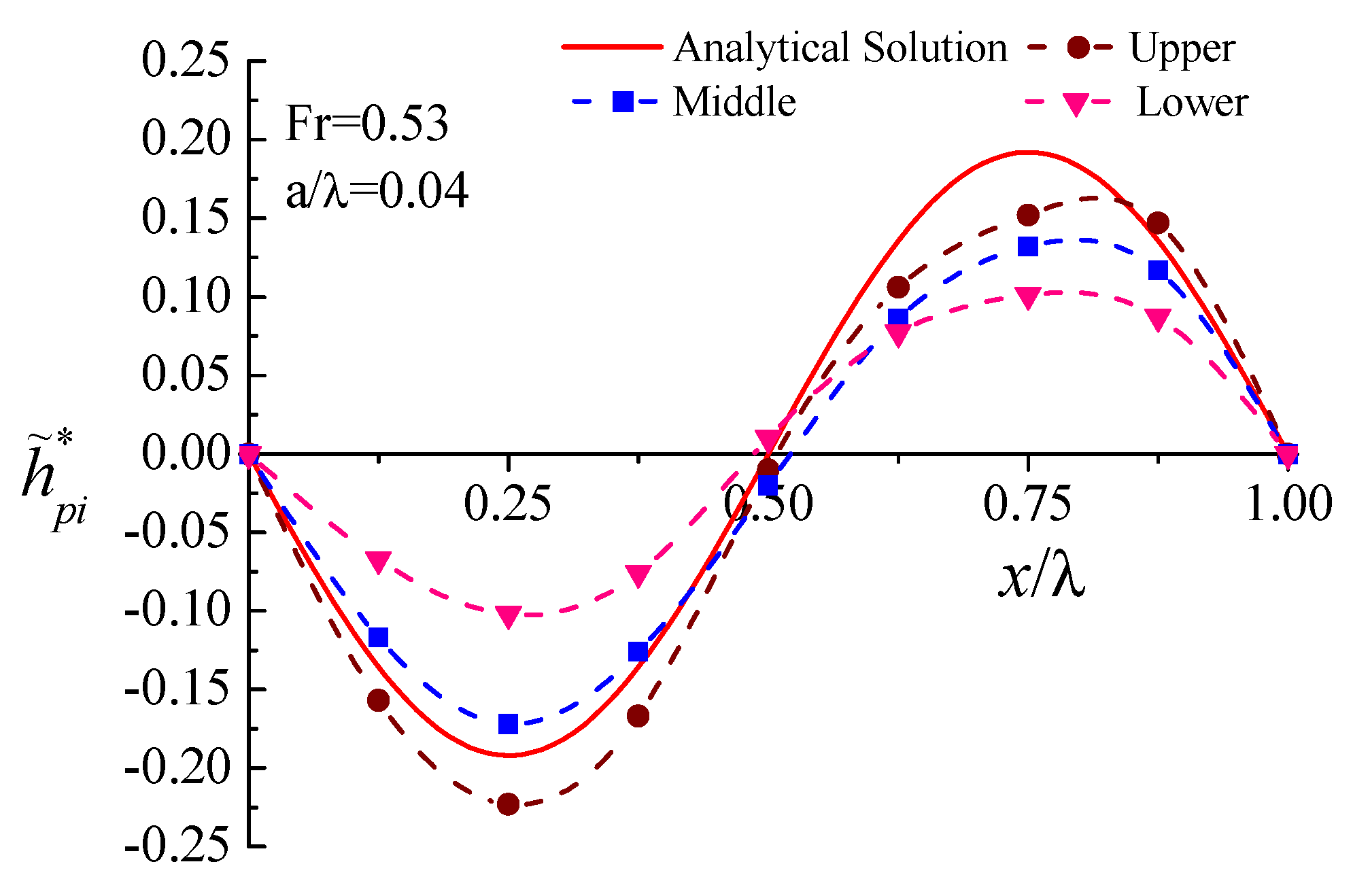
3.2. Experimental Results

For comparison, a dimensionless variable of water pressure head was defined as ${\tilde{h}}_{pi}^{*}=\frac{h_{pi}-h_{p0}}{u_{\infty }^2/2\mathrm{g}}$, where $h_{pi}$ is the measured water pressure head at the i^th section; $h_{p0}$ is the measured water pressure head at the 0λ section; u_∞ is the mean velocity of incoming flow. The water pressure heads of different layers on the slope of each cross section of experimental right segment under Fr = 0.53 and a/λ = 0.04 are presented in Figure 3, in which dashed lines dotted with round points, rectangle points and triangle points correspond to the upper, middle and lower layers, respectively. Meanwhile, we set the 0λ section as the original poin of x direction of analytical coordinate, and then the analytical pressures of this case are calculated by use of the Equation (28) and plotted in solid line in Figure 3.

Figure 3 shows that both outlines of the calculated and the measured water pressure heads roughly presented the same sinusoidal appearance as that of the bank form. The distribution pattern of water pressures was consistent with the variation tendency of the calculated curve, which indicated that the disturbed pressure heads along the sinusoidal bank-line also varied sinusoidally. In terms of the structure of the calculated and measured pressures in different slope positions, the best agreement was for the middle layer, while the greatest difference was for the lower part.

4. Discussion

4.1. Comparison Analysis and Discussion

As Figure 3 indicates that the relative agreement of analytical solutions and measured results has happened on the middle position of riparian slope, the experimental data on the middle position of riparian slope are selected for comparison analysis. The comparisons of analytical solutions with experimental data for the middle layer along the right bank under different run cases are plotted in Figure 4, in which red solid lines represent the analytical solutions that apply Equation (27) and blue dashed lines dotted with square points represent the measured data. Figure 4A–C show the comparisons under different Fr and the same a/λ, while Figure 4D–F express the comparisons under different a/λ. In general, the calculated magnitudes and structure of water pressures were in reasonable agreement with those of the measured water pressures in most run cases. In the convex region, the calculated pressures were slightly higher than the measurements. This was due to two possible reasons: (1) factually, there was secondary flow or more turbulent mixing in the experimental flume; (2) the actual roughness of the experimental boundaries had an effect on water pressure. However, in Run6 with a large a/λ, there was obvious disagreement. This implies that the analytical solution was unable to be fitted to flows with high curved boundaries.

Moreover, Figure 4 also illustrates the growth and decay tendency of water pressures along the alternating bends with the variation of Fr and sinuosity of the bank. When Fr increased from 0.4 to 0.65, the measured pressures became much closer and closer to the calculated pressures; see Figure 4A–C. Figure 4A–C also denote that the effect of Fr on the pressure variation was weak in the subcritical regime.

When a/λ increased from 0.04 to 0.16, the measured pressures became further and further away from the calculations; see Figure 4D–F. When a/λ was relatively small, the pressures reached trough and crest values at the convex and concave apexes, respectively. The reason might be that the water pressures within bending locations were mainly acted on by the centrifugal forces when the bank was low curved. This also verifies that the analytical solutions had a good agreement with experimental results under slightly curved cases. However, when a/λ was relatively large, the crest values of pressures began to move towards downstream and the trend lines of calculated pressures more and more obviously deviated from the measured trend lines. This phenomenon in Run6 was most remarkably demonstrated by the observation of flow separating from the bank in Run6, Figure 4F. Thus, it could be deduced that when the sinuosity of the bank increased to a certain critical value, the flow boundary layer might separate from the bank surface. Moreover, this could result in the main flow possibly being broken off near the back of the apex and forming inverse flow, making the main flow move towards the forehead of the apex. In this circumstance, the pressure distributions would depend on centrifugal forces, as well as the boundary layer separation and the main flow hitting. Therefore, unfortunately, the pressure expressions derived using small disturbance theory could not fit for the circumstance of drastic curved rivers.

4.2. Sensitivity Analysis and Discussion

In this section, the sensitivities of the water pressure heads to sinuosity, width and Fr have been analyzed. In this sensitivity analysis, the ranges of a/λ, b/λ and Fr were from 0 to 0.16, from 0 to 0.6 and from 0 to 0.9, respectively, the mid-values of which, i.e., 0.08, 0.3, 0.45, were set as the references. The variation ratios of water pressure heads, $R_{{\tilde{h}}_{pi}^{*}}$, responding to the variation ratios of a/λ, b/λ and Fr, i.e., $R_{\mathrm{a}/\mathsf{\lambda }}$, $R_{b/\mathsf{\lambda }}$, $R_{Fr}$, respectively, have been plotted in Figure 5, in which the sensitivities of $R_{{\tilde{h}}_{pi}^{*}}~R_{a/\mathsf{\lambda }}$, $R_{{\tilde{h}}_{pi}^{*}}~R_{b/\mathsf{\lambda }}$and $R_{{\tilde{h}}_{pi}^{*}}~R_{Fr}$ have been presented with a black solid line, red dashed line and blue dash-dot line, respectively.

As a/λ increased from the reference value 0.8 to 0.16 or decreased to 0, the variation ratio of a/λ was 100% or −100%, which resulted in the corresponding variation ratio of water pressure head $h_{pi}^{*}$ being also 100% or −100%. Additionally, the solid line in Figure 5 shows that the altitude of disturbed pressure was linear to a/λ and that they had same variation ratios. It is implied that a/λ played a significant role in the distribution of disturbed pressure.

When Fr increased from 0.45 to 0.9 with a 100% increase ratio, the variation ratio of disturbed pressure increased to 16.1%. On the other hand, while the variation ratio of Fr was −100%, that of the disturbed pressure was −4.2%. Note that there was no obvious variation of water pressure with the variation of Fr. In other words, Fr had unremarkable effects on the disturbed pressure distribution in subcritical flow (Fr < 1).

The red dashed line in Figure 5 shows that when b/λ was less than 0.8, the variation ratio of disturbed pressure was very obvious and approximately close to −100%. This indicates that b/λ had great influence on disturbed pressure as long as b/λ was small. In contrast, when b/λ was greater than 0.8 and its variation ratio increased, the variation ratio of disturbed pressure had no obvious increase. This means that when the river was wide, the disturbed pressure wave from one bankside was lightly weakened by the wave from the opposite side. Practically, the disturbed pressure wave driven by the bank form might travel in the cross-section direction and the energy of the wave might become weaker and weaker. If the edge forms of two bank sides were symmetrical, the phase displacement between disturbed pressure waves driven by the left bank and right bank was 180°. When the two waves met, the amplitude of the pressure wave from one side would be degraded by the one from the opposite side. Particularly, in a narrow river, the disturbed pressure wave from one bankside could be more strongly degraded by the one from the opposite side. This reasonably addresses why the greater b/λ had less effect on disturbed pressure than the smaller b/λ. When b/λ was greater than $2/\left(\mathsf{\pi }\mathsf{\omega }\right)$,$\frac{{\mathrm{e}}^{\frac{2\mathsf{\pi }\mathsf{\omega }\mathrm{b}}{\mathsf{\lambda }}}-1}{{\mathrm{e}}^{\frac{2\mathsf{\pi }\mathsf{\omega }\mathrm{b}}{\mathsf{\lambda }}}+1}$ approximately equalled to 1; thus, Equations (28) and (29) could be simplified again.

Right bank:

$${\tilde{h}}_{pi}^{*}=-\frac{4\mathsf{\pi }a}{\mathsf{\lambda }w}\cdot \sin \frac{2\mathsf{\pi }}{\mathsf{\lambda }}x$$

(30)

Left bank:

$${\tilde{h}}_{pi}^{*}=\frac{4\mathsf{\pi }a}{\mathsf{\lambda }w}\cdot \sin \frac{2\mathsf{\pi }}{\mathsf{\lambda }}x$$

(31)

5. Conclusions

In this study, the small-disturbance theory has been applied to derive the analytical solution of pressure distribution along a sinusoidal riverbank. Experiments have also been performed to test the hydrodynamic and geomorphic effects on pressure distribution and verified the applicability of the derived expressions. Based on these works, the following conclusions can be drawn.

The derived expressions of disturbed pressures, applying the approach of small-disturbance theory, were simple and accurate and agreed with experimental results for the riparian zones with low degree of curvature. Although assumptions and simplifications of small disturbance, potential flow, no flow separation and sinusoidal bank-line have been introduced in our formulation, the pressure expressions could still be used as a first order estimation for the disturbed pressure along a slightly curved riverbank.

On the contrary, when the riparian zones were highly-curved (i.e., a/λ was relatively big), the boundary layer could separate from the bank surface and the main flow could even hit the bank. The velocity field at the separation point or collision point changed sharply. Thus, the disturbances around these locations were relatively large and not significantly satisfied by using the basic assumptions of small-disturbance theory ($|\tilde{u}/u_{\infty }|\ll 1, |\tilde{v}/u_{\infty }|\ll 1$). Furthermore, in these cases, the calculation errors could also increase when the approximated boundary conditions on y = 0 and y = b (Equations (19) and (20)) were used as a surrogate for the real boundary conditions on a sinuous bank. Unfortunately, the pressure calculation approach based on small-disturbance theory could not effectively estimate the pressure distribution for a complex bank boundary or complex flow conditions.

Moreover, the analysis and derived expressions gave insight into the quantitative correlations between pressure variation and Froude number Fr, as well the ratio of bank amplitude to wavelength a/λ. The results of this study illustrated that the disturbed pressure along the riverbank increased as Fr or a/λ increased. Between these two factors, a/λ was found to conduct more significant influence on the pressure variation in subcritical flow.

References

1. Crowder, D.W. Reproducing and Quantifying Spatial Flow Patterns of Ecological Importance with Two-Dimensional Hydraulic Models. Ph.D. Thesis, Virginia Polytechnic Institute and State University, Blacksburg, VA, USA, 2002. [Google Scholar]
2. Peakall, J.; McCaffrey, B.; Kneller, B. A process model for the evolution and architecture of sinuous submarine channels. J. Sediment. Res. 2000, 70, 434–448. [Google Scholar] [CrossRef]
3. Kassem, A.; Imran, J. Three-dimensional modeling and analysis of density current, II. Flow in sinuous confined and unconfined channels. J. Hydraul. Res. 2004, 42, 591–602. [Google Scholar] [CrossRef]
4. Straub, K.M.; Mohrig, D.; Buttles, J.; McElroy, B.; Pirmez, C. Quantifying the influence of channel sinuosity on the depositional mechanics of channelized turbidity currents: A laboratory study. Mar. Pet. Geol. 2011, 28, 744–760. [Google Scholar] [CrossRef]
5. Kane, I.A.; McCaffery, W.D.; Peakall, J.; Kneller, B. Submarine channel levee shape and sediment waves from physical experiments. Sediment. Geol. 2010, 223, 75–85. [Google Scholar] [CrossRef]
6. Ezz, H.; Cantelli, A.; Imran, J. Experimental modeling of depositional turbidity currents in a sinuous submarine channel. Sediment. Geol. 2013, 290, 175–187. [Google Scholar] [CrossRef]
7. Buffington, J.; Tonina, D. Hyporheic exchange in mountain rivers, Part II: Effects of channel morphology on mechanics, scales, and rates of exchange. Geogr. Compass 2009, 3, 1038–1062. [Google Scholar] [CrossRef]
8. Tonina, D.; Buffington, J. Hyporheic exchange in mountain rivers, Part I: Mechanics and environmental effects. Geogr. Compass 2009, 3, 1063–1086. [Google Scholar] [CrossRef]
9. Wörman, A.; Packman, A.I.; Marklund, L.; Harvey, J.W.; Stone, S.H. Fractal topography and subsurface water flows from fluvial bedforms to the continental shield. Geophys. Res. Lett. 2007, 34. [Google Scholar] [CrossRef]
10. Stonedahl, S.H.; Harvey, J.W.; Worman, A.; Salehin, M. A multiscale model for integrating hyporheic exchange from ripples to meanders. Water Resour. Res. 2010, 46. [Google Scholar] [CrossRef]
11. Hicks, F.E.; Jin, Y.C.; Steffler, P.M. Flow near sloped bank in curved channel. J. Hydraul. Eng. 1990, 116, 55–70. [Google Scholar] [CrossRef]
12. Ghamry, H.K.; Steffler, P.M. Effect of applying different distribution shapes for velocities and pressure on simulation of curved open channels. J. Hydraul. Eng. 2002, 128, 969–982. [Google Scholar] [CrossRef]
13. Gholami, A.; Akhtari, A.A.; Minatour, Y.; Nonakdari, H.; Javadi, A.A. Experimental and numerical study on velocity fields and water surface profile in a strongly-curved 90° open channel bend. Eng. Appl. Comput. Fluid Mech. 2014, 8, 447–461. [Google Scholar] [CrossRef]
14. Pradhan, A.; Khatua, K.K.; Dash, S.S. Distribution of depth-averaged velocity along a highly sinuous channel. Aquat. Procedia 2015, 4, 805–811. [Google Scholar] [CrossRef]
15. Jin, Y.; Steffler, P.M.; Hicks, F.E. Roughness effects on flow and shear stress near outside bank of curved channel. J. Hydraul. Eng. 1990, 116, 563–577. [Google Scholar] [CrossRef]
16. Xia, J.; Lin, L.; Lin, J. Development of a GIS-based decision support system for diagnosis of river system health and restoration. Water 2014, 6, 3136–3151. [Google Scholar] [CrossRef]
17. Ghamry, H. Two dimensional vertically averaged and moment equations for shallow free surface flows. Ph.D. Thesis, University of Alberta, Edmonton Alta, AB, Canada, 1999. [Google Scholar]
18. Marzadri, A.; Tonina, D.; Bellin, A.; Tank, J.L. A hydrologic model demonstrates nitrous oxide emissions depend on streambed morphology. Geophys. Res. Lett. 2014, 41, 5484–5491. [Google Scholar] [CrossRef]
19. Tonina, D. Surface Water and Streambed Sediment Interaction: The Hyporheic Exchange. In Fluid Mechanics of Environmental Interfaces; Gualtieri, C., Mihailović, D.T., Eds.; CRC Press, Taylor & Francis Group: London, UK, 2012; pp. 255–294. [Google Scholar]
20. Lin, J. 3D numerical simulation of near-bank pressure field induced by sinuous bank morphology. In Proceedings of 35th IAHR World Congress on the Wise Find Pleasure in Water: Meandering Through Water Science and Engineering, Chengdu, China, 8–13 September 2013; Curran Associates Inc.: New York, NY, USA, 2014. [Google Scholar]
21. Singler, J.R. Transition to turbulence, small disturbances, and sensitivity analysis I: A motivating problem. J. Math. Anal. Appl. 2008, 337, 1425–1441. [Google Scholar] [CrossRef]
22. Trefethen, L.N.; Trefethen, A.E.; Reddy, S.C.; Driscoll, T.A. Hydrodynamic stability without eigenvalues. Science 1993, 261, 578–584. [Google Scholar] [CrossRef] [PubMed]
23. Silva, W.A.; Bennett, R.M. Using transonic small disturbance theory for predicting the aeroelastic stability of a flexible wind-tunnel model. NASA Technical Memo. 1990, 5. [Google Scholar] [CrossRef]
24. Hoefener, L.; Nitsche, W.; Carnarius, A.; Thiele, F. Experimental and numerical investigations of flow separation and transition to turbulence in an axisymmetric diffuser. In Proceedings of the 14th STAB/DGLR Symposium, New Results in Numerical and Experimental Fluid Mechanics V, Bremen, Germany, 16–18 November 2004; Rath, H.I., Holze, C., Heinemann, H.J., Henke, R., Hönlinger, H., Eds.; Springer-Verlag Berlin Heidelberg: Berlin, Germany, 2005. [Google Scholar]
25. Iatrou, M.; Breitsamter, C.; Laschka, B. Small disturbance Navier-Stokes equations: Application on transonic two-dimensional flows around airfoils. In Proceedings of the 14th STAB/DGLR Symposium, New Results in Numerical and Experimental Fluid Mechanics V, Bremen, Germany, 16–18 November 2004; Rath, H.I., Holze, C., Heinemann, H.J., Henke, R., Hönlinger, H., Eds.; Springer-Verlag Berlin Heidelberg: Berlin, Germany, 2005. [Google Scholar]
26. Liu, X. Open-Channel Hydraulics: From Then to Now and Beyond. In Handbook of Environmental Engineering; Wang, L.K., Yang, C.T., Eds.; Springer Science Business Media New York: New York, NY, USA, 2014; Volume 15, pp. 127–158. [Google Scholar]
27. Guo, Y.; Liu, R.; Duan, Y.; Li, Y. A characteristic-based finite volume scheme for shallow water equations. J. Hydrodyn. 2009, 21, 531–540. [Google Scholar] [CrossRef]
28. Xia, J.; Nehal, L. Hydraulic features of flow through emergent bending aquatic vegetation in the riparian zone. Water 2013, 5, 2080–2093. [Google Scholar] [CrossRef]
29. Tonina, D.; Buffington, J.M. Hyporheic exchange in gravel-bed rivers with pool-riffle morphology: Laboratory experiments and three-dimensional modeling. Water Resour. Res. 2007, 43. [Google Scholar] [CrossRef]
Figure 1. Schematic diagram of experimental setups. (A) is the view of the laboratory flume and measurement setups. (B) is the cross section of channel module; (C) is the top view of the sinusoidal river and test sections.
Water 08 00061 g001
Figure 2. Platform of a sinusoidal river and its coordinate system.
Water 08 00061 g002
Figure 3. Analytical solutions compared with experimental data in different layers under the Run2 case, in which the solid line represents the analytical solution, while dashed lines dotted with round points, rectangle points and triangle points correspond to the upper, middle and lower layers, respectively.
Water 08 00061 g003
Figure 4. Comparison of analytical solution and experimental data for middle layer under different run cases, in which solid line and dotted dashed line represent the analytical solutions and the experimental data, respectively.
Water 08 00061 g004
Figure 5. Sensitivity of the variation of water pressure head to that of a/λ, b/λ and Fr. The horizontal axis presents the variation ratios of a/λ, b/λ and Fr, while the vertical axis is the variation ratio of the water pressure head.
Water 08 00061 g005