Article

Spatio-Temporal Patterns and Source Identification of Water Pollution in Lake Taihu (China)

1
Department of Water Environmental Planning, Chinese Academy for Environmental Planning, Beijing 100012, China
2
Institute of Integrated Watershed Management, Laboratory for Earth Surface Processes, College of Urban and Environmental Sciences, Peking University, Beijing 100871, China
3
Laboratory of Land Surface Pattern and Simulation, Institute of Geographic Sciences and Natural Resources Research, Chinese Academy of Sciences, Beijing 100101, China
4
Center for Environmental Science, University of Maryland, Cambridge, MD 21613, USA
*
Author to whom correspondence should be addressed.
Water 2016, 8(3), 86; https://doi.org/10.3390/w8030086
Submission received: 8 December 2015 / Revised: 24 January 2016 / Accepted: 29 February 2016 / Published: 4 March 2016
(This article belongs to the Special Issue Lake Restoration and Management in a Climate Change Perspective)

Abstract

:
Various multivariate methods were used to analyze datasets of river water quality for 11 variables measured at 20 different sites surrounding Lake Taihu from 2006 to 2010 (13,200 observations), to determine temporal and spatial variations in river water quality and to identify potential pollution sources. Hierarchical cluster analysis (CA) grouped the 12 months into two periods (May to November, December to the next April) and the 20 sampling sites into two groups (A and B) based on similarities in river water quality characteristics. Discriminant analysis (DA) was important in data reduction because it used only three variables (water temperature, dissolved oxygen (DO) and five-day biochemical oxygen demand (BOD5)) to correctly assign about 94% of the cases and five variables (petroleum, volatile phenol, dissolved oxygen, ammonium nitrogen and total phosphorus) to correctly assign >88.6% of the cases. In addition, principal component analysis (PCA) identified four potential pollution sources for Clusters A and B: industrial source (chemical-related, petroleum-related or N-related), domestic source, combination of point and non-point sources and natural source. The Cluster A area received more industrial and domestic pollution-related agricultural runoff, whereas Cluster B was mainly influenced by the combination of point and non-point sources. The results imply that comprehensive analysis by using multiple methods could be more effective for facilitating effective management for the Lake Taihu Watershed in the future.

1. Introduction

The water quality in lakes has recently become a matter of great concern, because of its negative effects on human health and its contribution to harmful algal blooms. Accompanying the rapid growth of human population and industries, lake water is being heavily polluted from various sources, like domestic sewage, industrial wastewater, stormwater, agricultural runoff and atmospheric depositions [1,2,3,4]. Rivers, the natural pathways upstream of lakes, deliver most of the pollutant loadings into lakes [5,6]. To prevent and control lake water pollution, it is important to understand the temporal and spatial variations in upstream river water quality through routine monitoring programs. Currently, most monitoring programs generate datasets with information including physical properties, aggregate organic constituents and nutrients and inorganic constituents, making it difficult to analyze and interpret the underlying spatio-temporal patterns of water pollution [7,8]. Similarly, due to the complex interactions between natural processes and human activities, identifying potential pollution sources for river basins has also become a serious issue [7], which would eventually compromise the resilience and restoration of lakes.
Over the last decade, multivariate approaches have significantly advanced our understanding of the spatio-temporal patterns and pollution sources of river systems on the basis of water quality observations [8,9,10,11]. For instance, cluster analysis (CA), discriminant analysis (DA) and principal component analysis (PCA) have been widely used to assess spatial or temporal variations of groundwater and surface water quality [12,13,14,15,16]. However, reciprocal validation between any two multivariate analyses is still required to validate the results obtained by each approach [7]. Although the spatial and temporal variations of surface water quality in reservoirs or lakes have been extensively studied [17,18,19], how to identify the pollution sources for watershed systems still remains elusive due to the lack of pollution census data [20,21,22].
In this study, on the basis of a dataset obtained from a five-year (2006–2010) water-monitoring program in Lake Taihu Watershed in China, both CA and DA were performed to identify the spatio-temporal patterns in river water quality. PCA analysis was further performed to identify the underlying pollution sources in different regions. In the end, this study discussed the implications of local watershed management.

2. Materials and Methods

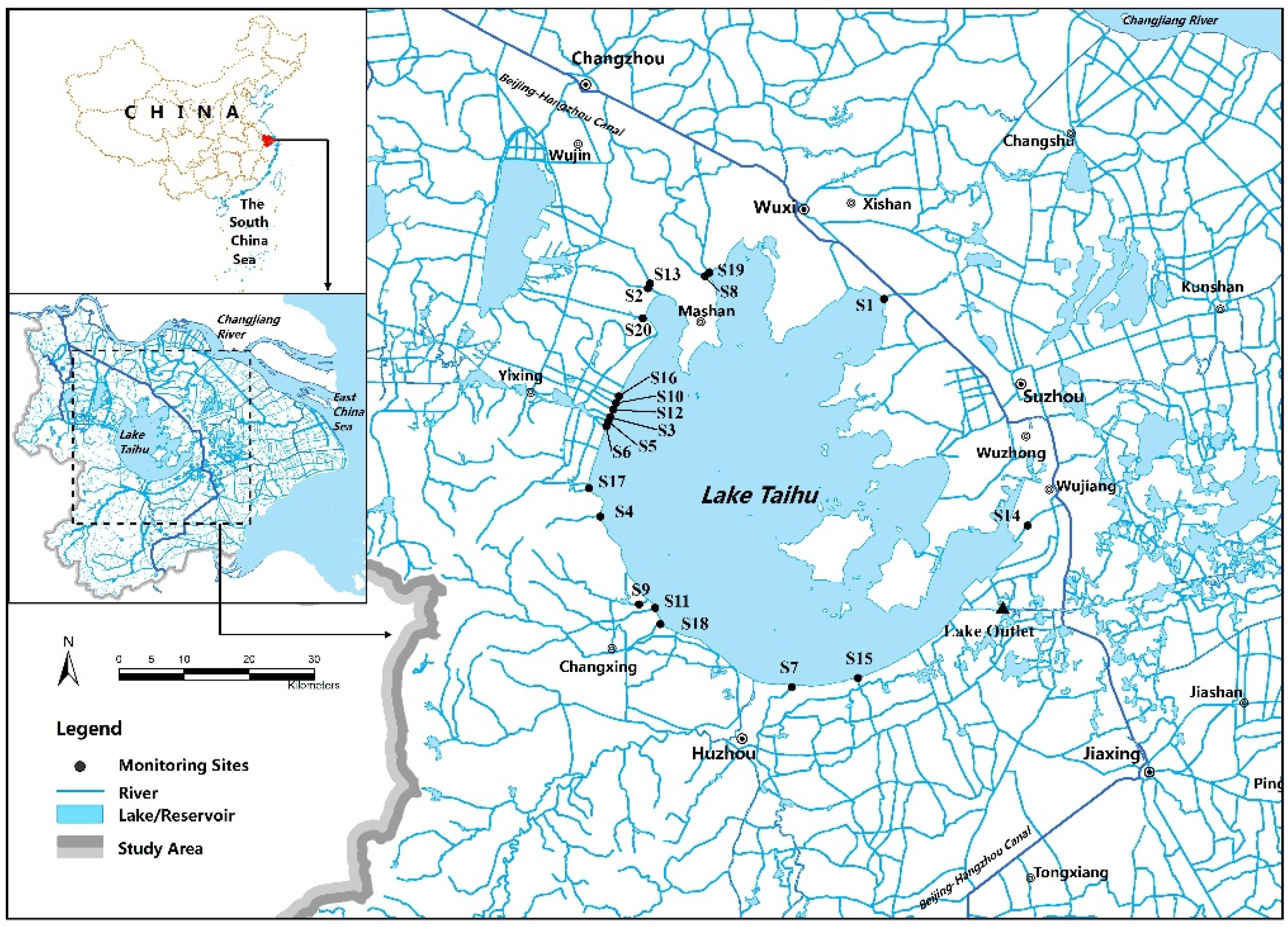
2.1. Study Area and Monitoring Program

Lake Taihu, the third largest freshwater lake in China, is situated in southeast Jiangsu Province and the lowest reach of the Yangtze River Basin, China (30°55′40′′–31°32′58′′ N; 119°52′32′′–120°36′10′′ E; Figure 1). The lake has a surface area of 2338 km2 with a maximum depth of 2.6 m and 1.9 m on average. The average water residence time is 309 days [23]. Lake Taihu is one of the main drinking water sources for neighboring residents, albeit one of the most heavily-polluted freshwater lakes in China [24]. Rapid economic expansion, population growth and industrial development surrounding Lake Taihu are accompanied with severe industrial pollution with a constant increase in domestic sewage and intensification of agricultural production [25,26], resulting in significant enrichment of organic substances and nutrients discharged into the surrounding riverine systems. This led to an overall decline in rivers’ water quality and ecosystem services in the Lake Taihu Watershed [27].
Water quality data was observed monthly between January 2006 and December 2010 at 20 monitoring sites in the rivers surrounding Lake Taihu (Figure 1), where the upstream catchment area and annual mean streamflow were illustrated in the Supplementary Material, Table S1. The monitored rivers contribute approximately 70% of total discharge into Lake Taihu [28]. Eleven water quality variables were selected for further analysis, i.e., water temperature (Temp), pH, conductivity (Cond), dissolved oxygen (DO), chemical oxygen demand (CODMn), five-day biochemical oxygen demand (BOD5), ammonium nitrogen (NH4+–N), total phosphorus (TP), total petroleum hydrocarbons (Petro), volatile phenol (V-ArOH) and plumbum (Pb). Other variables (e.g., cadmium, cuprum, cyanide) were not considered in this study, because their concentrations are less than the detection limits. Selected variables refer to physical properties, organic constituents, nutrient constituents or biological properties of the rivers (Table 1). Water samples were collected and analyzed by Environmental Monitoring Centers in Jiangsu and Zhejiang provinces. The water samples’ collection, preservation, transportation and analysis were performed according to the Technical Specifications Requirements for Monitoring of Surface Water and Wastewater of China. The analytical methods used in this study are also described in Table 1.

2.2. Multivariate Statistical Analysis

Spatio-temporal patterns in river water quality surrounding Lake Taihu were determined by CA using Ward’s method with squared Euclidean distance [7,29,30]. The linkage distance is expressed as (Dlink/Dmax) × 100, which represents the standardized quotient between the linkage distances for a particular case divided by maximal linkage distance [30]. DA was used in backward stepwise mode to confirm the groups found by CA and to evaluate the spatio-temporal variations of the discriminant variables. In DA, the monitoring period or site variables were the clustering variables, while the parameters from originally-measured datasets were independent [11,31]. Principal component analysis (PCA) is based on the assumption that there exists a bilinear model, which could explain the variance of observed water quality data by using less orthogonal variables, known as principal components [32]. Once Kaiser’s VARIMAX rotation is performed, factor loadings remain orthogonal and are no longer contributed to the explained maximum variance, while the scores become non-orthogonal. Using PCA, we could identify the unobservable latent pollution sources that affect the water quality of the upstream rivers. The details of multivariate analysis can be found in [30].

2.3. Data Pretreatment

The following data pretreatment methods were used for the river water quality dataset: (i) missing data were linearly interpolated based on the corresponding datasets; (ii) values below lower bounds were replaced with the mid-value between zero and the detection limit; (iii) the normality test was performed for each variable by analyzing its kurtosis and skewness, since most multivariate statistical analyses require the variables to be normally distributed. Unfortunately, skewness and kurtosis statistical test results suggest that most of the variables from the original data were severely deviated from the normal distribution at a confidence level of 95%. To satisfy the normality assumption, original data were logarithmically transformed, and further skewness and kurtosis values for the log-transformed data were significantly reduced and close to those for the normal distribution. All log-transformed variables were further z-scale standardized for CA and PCA analysis, while non-transformed original data were still used for DA analysis.

3. Results and Discussion

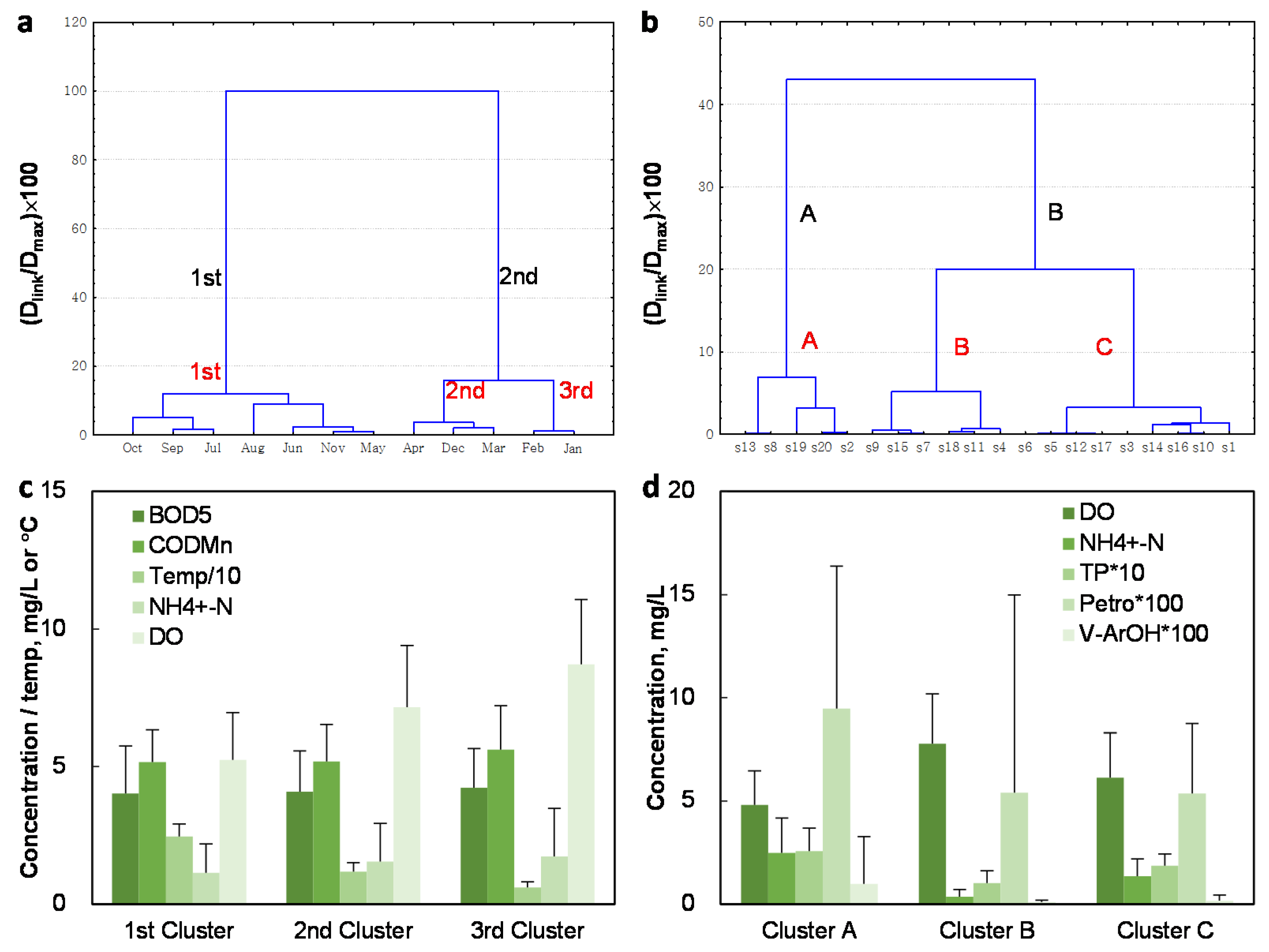
3.1. Temporal Similarity and Variation

Temporal hierarchical CA analysis generated a transient dendrogram and grouped the 12 months into either a two-cluster system at (Dlink/Dmax) × 100 < 20 or a three-cluster system at (Dlink/Dmax) × 100 < 16 (selecting the scale tree to (Dlink/Dmax) × 100 option in order for the tree plot to be scaled to a standardized scale). The temporal difference in water quality between the two systems was significant (Figure 2a; p < 0.01). In the two-cluster system, Cluster 1 (first period) covered the time from May to November while Cluster 2 (second period) ranged from December to the next April. In three-cluster system, while Cluster 1 remains the same as the previous system, Cluster 2 was further divided into two clusters: Cluster 2 for April, December and March and Cluster 3 for January to February (Figure 2a). Such a grouping differed from the Lake Dianchi Watershed, which is located in Southwest China [33], because the length of the wet season in the Lake Taihu Watershed (May to October) is much longer than the Lake Dianchi Watershed (July to September). In both two- and three-cluster systems, the temporal variations from river water quality data from Lake Taihu were determined by both hydrological condition (i.e., wet or dry season) and water pollution characteristics (Figure 2b). For example, NH4+–N in the first period (May to November) was much higher than the other clusters (Figure 2c), due to the greater contribution of agricultural runoff in the wet season. However, the mean concentrations of BOD5 and CODMn in the first period were close to the other two periods (Figure 2c), because the relatively larger amount of domestic sewage was offset by the greater streamflow in the rivers.
DA was then applied to evaluate the clusters’ systems generated by the temporal CA method. The objectives of the DA were to test the significance of discriminant functions and to choose the most significant variables that contributed to the differences among clusters. For each discriminant function, the results of Wilks’ lambda and chi-square analyses varied from 0.11 to 0.63 and 668 to 1972, respectively, with p < 0.001. This suggests that the temporal DA was reliable and effective [29,30]. In the two-cluster scenario, DA produced two classification matrices (CMs) with 94% accuracy of classification using three discriminant variables: water temperature, DO and BOD5 (Figure 2c). In the three-cluster scenario, DA produced three classification matrices (CMs) with 86.5% accuracy using two discriminant variables (i.e., CODMn and NH4+–N), which were significantly different from each other among the three-cluster systems (Figure 2c). For instance, the average means of the three variables (BOD5, CODMn and NH4+–N) in the third period were 3.4%, 8.4% and 12.5% higher than those of the second period (Figure 2c), respectively. The discrepancy between first and third period was similar to that between first and second period, whereas the gaps were much bigger for NH4+–N (Figure 2c). The two-cluster system divided the 12 months into wet and dry seasons, while the three-cluster system divided the 12 months into wet (May to November), moderate dry (March, April and December), severe dry seasons (January to February), according to local meteorological characteristics. Together, the backward stepwise DA results suggested that both two- and three-cluster systems explained the temporal similarities well. Water temperature, DO and BOD5 were the three most significant variables in discriminating the water quality condition in different seasons in both systems. Although the coefficient of variation (CV; Table 1) could reflect the numerical variations of samples, it is inappropriate to be used to evaluate the temporal variation among different seasons in either system.

3.2. Spatial Similarity and Variation

Through spatial CA analysis, we identified clusters of similar monitoring sites considering the effects of the temporal differences in spatial CA. Spatial similarity analysis was conducted for each individual temporal cluster, as well as all of the samples combined. Our results indicate that there were no significant differences among them, and further discussion will be focused on the spatial CA for all samples’ combined data. Spatial CA produced two dendrograms with two clusters at (Dlink/Dmax) × 100 < 20 and three clusters at (Dlink/Dmax) × 100 < 8, respectively. In the two-cluster dendrogram, Cluster A covered the S2, S8, S13, S19 and S20 sites, while Cluster B covered the S1, S3 to S7, S9 to S12 and S14 to S18 sites (Figure 2b). In the three-cluster dendrogram, Cluster B from the previous two-cluster dendrogram was further split into two clusters: new Cluster B with the S4, S7, S9, S11, S15 and S18 sites and new Cluster C with the rest of them (Figure 2b). All classifications varied at a significance level of p < 0.01, which meets our expectation, since the sites in the same cluster shared similar natural backgrounds and had been affected by similar sources in a similar way.
The spatial DA was performed similarly as the temporal DA (Table 2). We performed Wilks’ lambda and the chi-square analysis on each discriminant function. The values were within a range of 0.50 to 0.61 and 523 to 689, respectively, suggesting that the spatial DA had a similar discriminatory ability as the temporal DA. The spatial DA was performed using the original dataset with 11 variables after classifying into the two major groups (A and B) obtained from the spatial CA. Sites were the dependent variables, and the measured parameters were the independent variables. Backward mode discriminant functions successfully assigned >88.6% and >81.9% of the cases into the two- and three-cluster systems, respectively (Table 2). Moreover, the backward stepwise DA demonstrated that Petro, V-ArOH, DO, NH4+–N and TP were also significant discriminant variables for spatial variation (Figure 2d).
The sites in Cluster A were situated in the highly developed area (i.e., Wujin District or Xishan District of Changzhou City) (Figure 3), where most of the industrial effluents and domestic sewage flow into the rivers directly. Most of the sites in Cluster B were located in the Tiaoxi River Basin (Figure 3). Tiaoxi River is the largest tributary of Lake Taihu, and it originates from mountainous area and moderately developed rural regions. The sites in Cluster C were located in northwestern and eastern Lake Taihu (Figure 3) in Yixing City and Wuzhong District of Suzhou City, where the major pollution sources include both point and non-point sources.

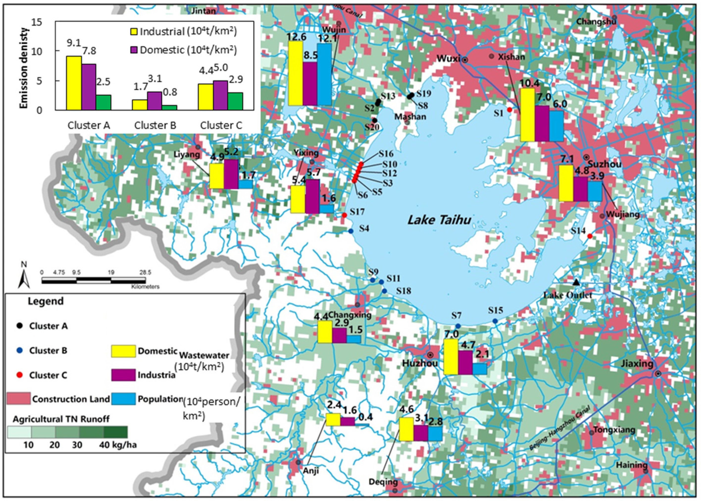
3.3. Identification of Potential Pollution Sources

Due to the similarity between two- and three-cluster systems (see Supplementary Material, Table S2), source identification of water pollution for the two-cluster system was only illustrated. Before conducting the PCA analysis, the Kaiser-Meyer-Olkin (KMO) and Bartlett’s sphericity tests were performed on the parameter correlation matrix. The KMO results for Clusters A and B were 0.56 and 0.52, respectively, and Bartlett’s sphericity results were 861 and 812 (p < 0.05), indicating that PCA could be used in dimensionality reduction. PCAs were applied to standardized log-transformed datasets (11 variables) to examine the differences between Clusters A and B and to identify the latent factors. PCA with VARIMAX rotation explained 75.6% and 67.0% of the total variance in Clusters A and B, respectively (Table 3). Such a performance of source identification was close to those for Lake Dianchi and Lake Chaohu in China [33,34].
For Cluster A, the first varifactor (VF1), which explained 18.6% of the total variance, had only strong positive loadings on Petro and Pb, but a moderate loading on V-ArOH (Table 3). The element Pb is mainly from electronic manufacturing and chemical industries; V-ArOH is from paper-making and chemical industries; and Petro is from equipment manufacturing, metal smelting industries and chemical industries. VF1 represented chemical pollution, which is originated from industrial wastewater and discharged into the rivers. VF2 represented domestic pollution, explaining 17.09% of the total variance, and had strong positive loadings on TP, CODMn and BOD5. VF3 could be interpreted as N-related industrial pollution, which accounted for 16.7% of the total variance and had strong positive loadings on conductivity (Cond) and NH4+–N. VF4 and VF5 explained 13.29% and 9.97% of the total variance, respectively. VF4 had strong positive loadings on water temperature, but strong negative loadings on DO, while VF5 had only strong positive loadings on pH. VF5 was attributed to the variability from the physicochemical source and represented natural sources impacted by seasonality.
According to the Pollution Source Census Survey of Jiangsu and Zhejiang provinces, V-ArOH, identified in VF1, is majorly generated by chemical manufactures in Lake Taihu area, and approximately 35% of V-ArOH is from the Wujin District of Changzhou City (Figure 3), a Cluster A catchment area. Major chemical manufactures in Wujin District were under tight regulation by local government, but the total V-ArOH discharge is still massive. Moreover, 89% of Pb discharge was from communication and electronic manufactures that are widely spread in the Class A catchment areas in Wujin District of Changzhou City and Xishan District of Wuxi City. Similarly, petroleum-related emissions are also from electronic manufacturing and chemical industries.
Since urbanization expansion was accompanied with population growth, domestic pollution became the primary source and is represented by VF2 (Table 3), with the major factors of TP, CODMn and BOD5. High population density could lead to massive organic pollution without proper regulation. In the Class A catchment area, the population density reached 1148 persons/km2, and industrial wastewater discharge density was close to 90,000 tons/km2 annually (Figure 3) Moreover, agricultural runoff of TN was 2.5 tons/km2 annually. Therefore, domestic pollution in this area is becoming a serious issue and should be carefully considered within the pollution control plan in the future.
Further analysis of VF3 from historic statistical data suggests that nitrogen (N) emission was primarily from industrial wastewater. In the Cluster A catchment area, 55% of NH4+–N was from industrial wastewater, which is moderately correlated with V-ArOH, 31% from agricultural runoff and 14% from domestic sewage. Since the combined N emissions affect electronic conductivity, the potential pollution source VF3 could also be explained as N-related industrial pollution.
For Cluster B, VF1 (accounting for 27.14% of the total variance) had strong positive loadings on CODMn, TP, NH3+–N, conductivity and BOD5, which represent the combination of point and non-point sources. For instance, domestic wastewater discharge per area in Cluster B was only 34,000 tons/km2 annually, which is less than half that in Cluster A (Figure 3). However, agricultural runoff of TN was up to 2.9 tons/km2 annually, close to the intensity of that in Cluster A (Figure 3). As previously mentioned, VF2 explained 14.3% of the total variance and had positive loadings on water temperature, but strongly negative on DO. It represented natural sources impacted by seasonal change and hydrological conditions (Singh et al. [29]; Zhou et al., [26]). VF3 (13.77% of the total variance) was positively weighted by petroleum-related pollutions and had negative loadings on pH. Previously, we demonstrated that petroleum-related emissions were from multiple industries and represented the intensity of industrial development in a certain area. VF4 explained 11.7% of the total variance and had strong positive loadings on Pb and V-ArOH. Similar to the Cluster A area, VF4 was categorized as a chemical-related industrial pollution factor. Pb and V-ArOH discharges were mainly from electronic and chemical manufactures. However, it was still considered as an independent impact factor due to continuing economic growth and industrial development in this area.
Analysis of the major factors and main pollution patterns in the highly-polluted area (Class A area) and the moderately-polluted area (Class B area) revealed that there were significant differences between these two groups. The Cluster A area was severely impacted by the heavy chemical industries. Recently, the Cluster A area performed better in controlling pollution under strong regulations and pollution control. Pb and V-ArOH levels were basically below the detection limits. Nevertheless, due to the huge total discharge amount, stronger regulations and pollution controls would be still required to reduce emission amounts from chemical manufacturing, electronic and communication manufactures, compared to current conditions. The most prominent source in the Cluster B area was domestic pollution, whereas industrial pollution, as an independent major factor, could not be ignored either. Moreover, since natural conditions are the second important pollution factor in this area, different seasons with distinct precipitation would result in different lake water quality.

4. Conclusions and Implications

Multivariate statistical methods were successfully applied to evaluate temporal and spatial variations in studying river water quality and identifying pollutions sources at river outlets surrounding Lake Taihu Watershed. Our results suggest that multiple methods are effective and compatible with each other and could be used in river water quality management in the future. Hierarchical CA clustered the 12 months into three periods and classified 16 sampling sites into two groups (A and B) based on the similarity of water quality characteristics. Both temporal and spatial DA analysis had the best performance with good discriminatory ability according to significance validation tests. They also identified several significant variables for discrimination among temporal or spatial groups. Analysis of temporal variation by DA required only three variables, but successfully assigned about 94% of the cases, and analysis of spatial variation required only five variables, but with more than 88.6% cases successfully assigned. In conclusion, the temporal and spatial similarities and differences could optimize monitoring programs with decreased monitoring frequency and a decreased number of sampling monitoring stations and monitoring variables, which could finally significantly reduce the subsequent costs. Moreover, PCA analysis identified four and five latent pollution sources for Clusters A and B, respectively, which are industrial source (chemical-related, petroleum-related or N-related), domestic source, a combination of point and non-point sources and natural source. Overall, our study provides important information in the understanding and characterization of pollution patterns surrounding the Lake Taihu area. However, how to accurately quantify the contributions of different pollution resources still remains elusive. Future study needs supplemental investigations on potential pollution resources and continuing monitoring of upstream rivers. Furthermore, comprehensive analysis in combination by using multiple methods could be more effective for facilitating effective management for the Lake Taihu Watershed in the future.

Supplementary Files

Supplementary File 1

Acknowledgments

This study was funded by the National Water Science and Technology Research Project (2013ZX07102-006), the National Natural Science Foundation of China (No. 41201077), the Research Fund for the 111 Project (No. B14001). We also thank two native English speakers from Z & Z Consultant LLC for their editing services on the manuscript.

Author Contributions

Feng Zhou and Yan Chen conceived and designed the experiments; Yan Chen, Kangping Zhao, Yueying Wu, Shuoshuo Gao, Wei Cao, Yan Bo, Ziyin Shang, Jing Wu and Feng Zhou analyzed the data; F.Z. and Y.C. wrote the paper.

Conflicts of Interest

The authors declare no conflict of interest.

References

  1. Nyairo, W.N.; Owuor, P.O.; Kengara, F.O. Effect of anthropogenic activities on the water quality of Amala and Nyangores tributaries of River Mara in Kenya. Environ. Monit. Assess. 2015, 187, 1–12. [Google Scholar] [CrossRef] [PubMed]
  2. Niu, Y.; Niu, Y.; Pang, Y.; Yu, H. Assessment of Heavy Metal Pollution in Sediments of Inflow Rivers to Lake Taihu, China. Bull. Environ. Contam. Toxicol. 2015, 95, 618–623. [Google Scholar] [CrossRef] [PubMed]
  3. Huang, K.; Guo, H.; Liu, Y.; Zhou, F.; Yu, Y.; Wang, Z. Water environmental planning and management at the watershed scale: A case study of Lake Qilu, China. Front. Environ. Sci. Eng. China 2008, 2, 157–162. [Google Scholar] [CrossRef]
  4. Bozelli, R.L.; Caliman, A.; Guariento, R.D.; Carneiro, L.S.; Santangelo, J.M.; Figueiredo-Barros, M.P.; Leala, J.J.F.; Rocha, A.M.; Quesado, L.B.; Lopes, P.M.; et al. Interactive effects of environmental variability and human impacts on the long-term dynamics of an Amazonian floodplain lake and a South Atlantic coastal lagoon. Limnologica 2009, 39, 306–313. [Google Scholar] [CrossRef]
  5. Chen, K.; Wang, X.; Li, D.; Li, Z. Driving force of the morphological change of the urban lake ecosystem: A case study of Wuhan, 1990–2013. Ecol. Model. 2015, 318, 204–209. [Google Scholar] [CrossRef]
  6. Zhou, F.; Liu, Y.; Guo, H. Application of multivariate statistical methods to water quality assessment of the watercourses in northwestern new territories, Hong Kong. Environ. Monit. Assess. 2007, 132, 1–13. [Google Scholar] [CrossRef] [PubMed]
  7. Li, X.; Li, P.; Wang, D.; Wang, Y. Assessment of temporal and spatial variations in water quality using multivariate statistical methods: A case study of the Xin’anjiang River, China. Front. Environ. Sci. Eng. 2014, 8, 895–904. [Google Scholar] [CrossRef]
  8. Yang, Y.H.; Zhou, F.; Guo, H.C.; Sheng, H.; Liu, H.; Dao, X.; He, C.J. Analysis of spatial and temporal water pollution patterns in Lake Dianchi using multivariate statistical methods. Environ. Monit. Assess. 2010, 170, 407–416. [Google Scholar] [CrossRef] [PubMed]
  9. Magyar, N.; Hatvani, I.G.; Székely, I.K.; Herzig, A.; Dinka, M.; Kovács, J. Application of multivariate statistical methods in determining spatial changes in water quality in the Austrian part of Neusiedler See. Ecol. Eng. 2013, 55, 82–92. [Google Scholar] [CrossRef]
  10. Singh, U.B.; Ahluwalia, A.S.; Jindal, R.; Sharma, C. Water Quality Assessment of Some Freshwater Bodies Supporting Vegetation in and Around Chandigarh (India), Using Multivariate Statistical Methods. Water Qual. Expo. Health 2013, 5, 149–161. [Google Scholar] [CrossRef]
  11. Jiang, Y.; Guo, H.; Jia, Y.; Cao, Y.; Hu, C. Principal component analysis and hierarchical cluster analyses of arsenic groundwater geochemistry in the Hetao basin, Inner Mongolia. Chem. Erde Geochem. 2015, 75, 197–205. [Google Scholar] [CrossRef]
  12. Sinha, K.; Das Saha, P. Assessment of water quality index using cluster analysis and artificial neural network modeling: A case study of the Hooghly River basin, West Bengal, India. Desalin. Water Treat. 2015, 54, 28–36. [Google Scholar] [CrossRef]
  13. Kim, S.W.; Park, J.S.; Kim, D.; Oh, J.M. Runoff characteristics of non-point pollutants caused by different land uses and a spatial overlay analysis with spatial distribution of industrial cluster: A case study of the Lake Sihwa watershed. Environ. Earth Sci. 2014, 71, 483–496. [Google Scholar] [CrossRef]
  14. Kamble, S.R.; Vijay, R. Assessment of water quality using cluster analysis in coastal region of Mumbai, India. Environ. Monit. Assess. 2011, 178, 321–332. [Google Scholar] [CrossRef] [PubMed]
  15. Yerel, S.; Anagun, A.S. Assessment of water quality observation stations using cluster analysis and ordinal logistic regression technique. Int. J. Environ. Pollut. 2010, 42, 344–358. [Google Scholar] [CrossRef]
  16. Ban, X.; Wu, Q.; Pan, B.; Du, Y.; Feng, Q. Application of Composite Water Quality Identification Index on the water quality evaluation in spatial and temporal variations: A case study in Honghu Lake, China. Environ. Monit. Assess. 2014, 186, 4237–4247. [Google Scholar] [CrossRef] [PubMed]
  17. Cid, F.D.; Antón, R.I.; Pardo, R.; Vega, M.; Caviedes-Vidal, E. Modelling spatial and temporal variations in the water quality of an artificial water reservoir in the semiarid Midwest of Argentina. Anal. Chim. Acta 2011, 705, 243–252. [Google Scholar] [CrossRef] [PubMed]
  18. Varol, M.; Gökot, B.; Bekleyen, A.; Şen, B. Spatial and temporal variations in surface water quality of the dam reservoirs in the Tigris River basin, Turkey. Catena 2012, 92, 11–21. [Google Scholar] [CrossRef]
  19. Guo, H.C.; Liu, L.; Huang, G.H.; Fuller, G.A.; Zou, R.; Yin, Y.Y. A system dynamics approach for regional environmental planning and management: A study for the Lake Erhai Basin. Environ. Manag. 2001, 61, 93–111. [Google Scholar] [CrossRef] [PubMed]
  20. Liu, Y.; Guo, H.; Yu, Y.; Dai, Y.; Zhou, F. Ecological-economic modeling as a tool for watershed management: A case study of Lake Qionghai watershed, China. Limnologica 2008, 38, 89–104. [Google Scholar] [CrossRef]
  21. Qin, B.; Xu, P.; Wu, Q.; Luo, L.; Zhang, Y. Environmental issues of Lake Taihu, China. Hydrobiologia 2007, 581, 3–14. [Google Scholar] [CrossRef]
  22. Shen, P.P.; Shi, Q.; Hua, Z.C.; Kong, F.X.; Wang, Z.G.; Zhuang, S.X.; Chen, D.C. Analysis of microcystins in cyanobacteria blooms and surface water samples from Meiliang Bay, Taihu Lake, China. Environ. Int. 2003, 29, 641–647. [Google Scholar] [CrossRef]
  23. Qin, B.Q.; Zhu, G.; Gao, G.; Zhang, Y.; Li, W.; Paerl, H.W.; Carmichael, W.W. A drinking water crisis in Lake Taihu, China: Linkage to climatic variability and lake management. Environ. Manag. 2010, 45, 105–112. [Google Scholar] [CrossRef] [PubMed]
  24. Bai, X.; Ding, S.; Fan, C.; Liu, T.; Shi, D.; Zhang, L. Organic phosphorus species in surface sediments of a large, shallow, eutrophic lake, Lake Taihu, China. Environ. Pollut. 2009, 157, 2507–2513. [Google Scholar] [CrossRef] [PubMed]
  25. Zhou, F.; Guo, H.; Hao, Z. Spatial distribution of heavy metals in Hong Kong’s marine sediments and their human impacts: A GIS-based chemometric approach. Mar. Pollut. Bull. 2007, 54, 1372–1384. [Google Scholar] [CrossRef] [PubMed]
  26. Zhou, F.; Huang, G.H.; Guo, H.; Zhang, W.; Hao, Z. Spatio-temporal patterns and source apportionment of coastal water pollution in eastern Hong Kong. Water Res. 2007, 41, 3429–3439. [Google Scholar] [CrossRef] [PubMed]
  27. Wang, H.; Wang, C.; Wu, W.; Mo, Z.; Wang, Z. Persistent organic pollutants in water and surface sediments of Taihu Lake, China and risk assessment. Chemosphere 2003, 50, 557–562. [Google Scholar] [CrossRef]
  28. Yan, S.W.; Yu, H.; Zhang, L.; Xu, J.; Wang, Z. Water quantity and pollutant fluxes of inflow and outflow rivers of Lake Taihu, 2009. J. Lake Sci. 2011, 23, 855–862. (In Chinese) [Google Scholar]
  29. Singh, K.P.; Malik, A.; Mohan, D.; Sinha, S. Multivariate statistical techniques for the evaluation of spatial and temporal variations in water quality of Gomti River (India)—A case study. Water Res. 2004, 38, 3980–3992. [Google Scholar] [CrossRef] [PubMed]
  30. Pekey, H.; Karakas, D.; Bakoglu, M. Source apportionment of trace metals in surface waters of a polluted stream using multivariate statistical analyses. Mar. Pollut. Bull. 2004, 49, 809–818. [Google Scholar] [CrossRef] [PubMed]
  31. Zhou, F.; Shang, Z.Y.; Ciais, P.; Tao, S.; Piao, S.L.; Raymond, P.; He, C.F.; Li, B.G.; Wang, R.; Wang, X.H.; et al. A new high-resolution N2O emission inventory for China in 2008. Environ. Sci. Technol. 2014, 48, 8538–8547. [Google Scholar] [CrossRef] [PubMed]
  32. Hou, X.K.; Zhou, F.; Leip, A.; Fu, B.J.; Yang, H.; Chen, Y.; Gao, S.S.; Shang, Z.Y. Precipitation and clay content explain half of nitrogen runoff variability in Chinese paddy fields. Agric. Ecosyst. Environ. 2015. submitted. [Google Scholar]
  33. Yang, Y.; Wang, C.; Guo, H.; Sheng, H.; Zhou, F. An integrated SOM-based multivariate approach for spatio-temporal patterns identification and source apportionment of pollution in complex river network. Environ. Pollut. 2012, 168, 71–79. [Google Scholar] [CrossRef] [PubMed]
  34. Xu, Y.; Ma, C.; Huo, S.; Xi, B.; Qian, G. Performance assessment of water quality monitoring system and identification of pollution source using pattern recognition techniques: A case study of Chaohu Lake, China. Desalin. Water Treat. 2012, 47, 182–197. [Google Scholar] [CrossRef]
Figure 1. Study area and its monitoring sites.
Water 08 00086 g001
Figure 2. Temporal and spatial similarities of monitoring periods or sites produced by cluster analysis (CA). The values for water temperature, TP, Petro and V-ArOH are re-scaled by multiplying by 0.1, 10, 100 and 100. The units for concentration or temperature are mg/L and °C. (a) Dendrogram for temporal similarity of monitoring periods; (b) Dendrogram for spatial similarity of monitoring sites; (c) Differences in discriminant variables among two-cluster system; (d) Same as panel c but for three-cluster system.
Water 08 00086 g002
Figure 3. Spatial pattern of the grouping of monitoring sites and the corresponding emission rates per area of industrial source, domestic source and agricultural runoff. The grouping is determined by the three-cluster systems. The wastewater amounts of industrial and domestic pollution sources are extracted from the Pollution Source Census Survey of Jiangsu and Zhejiang provinces for the period pf 2007 to 2010, while the agricultural runoff of TN is obtained from Zhou et al. [31] and Hou et al. [32]. The emission density of individual pollution sources in each cluster is shown in the inset of the top-left of the map.
Water 08 00086 g003
Table 1. Univariate statistics and analytical methods in the analysis of the water quality variables for rivers surrounding Lake Taihu. SD and CV stand for standard deviation and coefficient of variation, respectively. Temp, temperature; Cond, conductivity; DO, dissolved oxygen; CODMn, chemical oxygen demand; BOD5, chemical oxygen demand; TP, total phosphorus; Petro, total petroleum hydrocarbons; V-ArOH, volatile phenol.
VariableMeanMinMaxSDCVAnalytical Method *
Temp (°C)18.322.1034.108.5646.70Thermometer
pH7.476.258.910.334.49Glass electrode
Cond (ms/m)63.6910.70794.0037.7259.22Electrical conductivity meter
DO (mg/L)6.300.6013.382.3938.01Iodometric
CODMn (mg/L)5.250.6013.801.3124.92Potassium permanganate method
BOD5 (mg/L)4.080.6014.401.6239.63Dilution and inoculation test
NH4+–N (mg/L)1.350.0115.401.3096.41N-reagent colorimetry
TP (mg/L)0.180.010.960.0953.10Ammonium molybdate spectrophotometry
Petro (mg/L)0.060.010.960.07107.94Infrared spectrophotometric method
V-ArOH (mg/L)0.000.000.310.01338.71Spectrophotometric determination with 4-amino-antipyrin
Pb (mg/L)0.010.000.040.01107.34Atomic absorption spectrophotometry
Note: * The details of the analytical methods can be found in the Technical Specifications Requirements for Monitoring of Surface Water and Wastewater of China.
Table 2. Classification matrices for backward discriminant analysis (DA) of temporal and spatial variations.
No. of ClustersGroupTemporal VariationSpatial Variation
% Correct1st2nd3rd% Correct1st2nd3rd
Two clusters1st93.576554595.2285743
2nd94.602747369.0093207
Total94.0068251888.67950250
Three clusters1st91.8664357084.72305253
2nd80.67222423669.67120990
3rd76.5004715386.852546469
Total86.5066534618981.92331257612
Table 3. Loadings of 11 measured variables on VARIMAX rotated factors of two clusters.
VariablesVFs for Cluster AVFs for Cluster B
123451234
Petro0.820.13−0.090.00−0.140.05−0.010.740.17
Pb0.82−0.060.15−0.02−0.09−0.05−0.02−0.050.83
V-ArOH0.480.350.480.03−0.010.230.010.090.69
TP0.060.790.220.01−0.220.820.030.110.05
CODMn0.120.710.320.100.300.830.10−0.060.14
BOD5−0.600.64−0.03−0.05−0.020.690.080.310.16
Cond−0.010.110.85−0.09−0.130.690.02−0.08−0.07
NH4+–N0.070.230.800.120.220.72−0.050.440.12
DO−0.14−0.20−0.140.89−0.05−0.30−0.83−0.23−0.07
Temp−0.17−0.31−0.19−0.80−0.05−0.120.92−0.09−0.07
pH−0.20−0.040.02−0.020.93−0.10−0.11−0.770.16
Eigenvalue2.041.881.841.461.102.991.581.511.29
% Total variance18.5817.0916.7013.299.9727.1414.3313.7711.72
Cumulative % variance18.635.752.465.775.627.141.555.267.0

