Abstract
One of the challenges faced by subwatershed hydrology is the discovery of patterns associated with climate and landscape variability with the available data. This study has three objectives: (1) to evaluate the annual recession curves; (2) to relate the recession parameter (RP) with physiographic characteristics of 21 Mexican subwatersheds in different climate regions; and (3) to formulate a Baseflow (BF) model based on a top-down approach. The RP was calibrated utilizing the largest magnitude curves. The RP was related to topographical, climate and soil variables. A non-linear model was employed to separate the baseflow which considers RP as a recharge rate. Our results show that RP increases with longitude and decreases with latitude. RP displayed a sustained non-linear behavior determined by precipitation rate and evapotranspiration () over years and subwatersheds. The model was fit to a parameter concurrent with invariance and space-time symmetry conditions. The dispersion of our model was associated with the product of () by the aquifer’s transmissivity. We put forward a generalized baseflow model, which made the discrimination of baseflow from direct flow in subwatersheds possible. The proposed model involves the recharge-storage-discharge relation and could be implemented in basins where there are no suitable ground-based data.
1. Introduction
Baseflow (BF) is an essential component for the hydrological balance of a basin. Its study is necessary for different purposes, such as aquatic systems’ preservation, hydroelectric energy generation and pollutant transportation, and it also includes the effects of plant coverage changes on surface runoff [,,]. Long-term hydrological balance within the basin depends on water and energy availability []. Budyko’s model considers this relation and associates actual and potential evapotranspiration (energy) with precipitation (water). This model and its derivations have been proven reliable through validation in different climate and physiographic conditions around the world [,,,].
This approach has been utilized to predict BF; for instance, Wang and Luo [] found an association between the aridity index and perennial stream. The baseflow recession parameter (RP) has also been related by means of this model; van Dick [] noted how the parameter decreased exponentially as the aridity index value increased. Furthermore, Beck et al. [] observed the same trend when they correlated climate, topography, plant coverage, geology and soil type with the baseflow recession parameter. Their results indicated non-linear and heteroscedastic relations with satisfactory fits (R2 > 0.72). Similar studies associated the baseflow index with geographical, climate and edaphic patterns [,].
This model has the disadvantage of disregarding underwater storage, making it impractical to model the water balance at temporal scales []. According to Istambulluoglu et al. [], the model correlates negatively as the aridity index increases, which points out the need to include the baseflow component into Budyko-like hydrological balances on an interannual basis.
Other studies have described how hydrological balance variability and interaction within and among subwatersheds follow similar patterns []. For instance, the precipitation-runoff relations on a monthly and an annual basis tend to display non-linear behaviors, varying only in magnitude, as shown by Ponce and Shetty []. These studies describe a space-time dependence that can be labeled as symmetry, where observations from different regions can be utilized for the construction of a generalized model with invariance principles [,]. The recession master curve is a symmetric model for studying BF; however, according to Tallaksen [], it is inconvenient due to its grouping of n different recession curves along the year, a procedure that turns out to be time consuming if many years are to be analyzed.
Although there are simplifications based on linear reservoirs utilized to separate baseflow [,], the linear algorithm can only be successful when short periods of recession are adjusted. According to He et al. [], in most cases of unconfined aquifers, the storage-discharge relationship in an aquifer represented by the curve of recession is set to a concave shape, indicating the non-linearity of the process.
Moreover, the problem of calibrating and validating mechanistic models in Mexico is that there is not enough data to feed these models []. Therefore, this research aimed at discovering new hydrological patterns that incorporate within them the effects of the natural heterogeneity found in different subwatersheds [], responding to the hypothesis of a robust hydrological model, sustained on physical limits and based on easily accessible data that can be replicated in any zone.
Therefore, the proposal of this study can be divided into three different objectives. The first one was to evaluate the annual recession curve with a non-linear model; the second one was to relate the recession parameter with subwatershed physiographics; and the last one was to formulate a baseflow model supported by the symmetry and invariance principles. Our base hypothesis was that working with annual data enables a separation of baseflow into shorter time scales.
2. Materials and Methods
2.1. Input Data
Daily runoff registers (converted into mm·d−1) from 21 Mexican subwatersheds were gathered; the source of this information was El Banco Nacional de Datos de Aguas Superficiales []. The subwatersheds were selected so as to represent different climate characteristics (aridity index, seasonality, humidity), as shown by Garcia et al. [], and landscape characteristics (topography, soil and plant coverage).
An additional criterion was that the subwatersheds were located in National Parks and Biosphere Reserves, in order to avoid as much as possible extraneous influences on the hydrological regime (water extraction, urban development, storage works, etc.) (Figure 1). The subwatersheds areas ranged from 42 to 23,475 km2. The analyzed period went from 1950 to 2011, which is the period of available hydrometric data in Mexico.
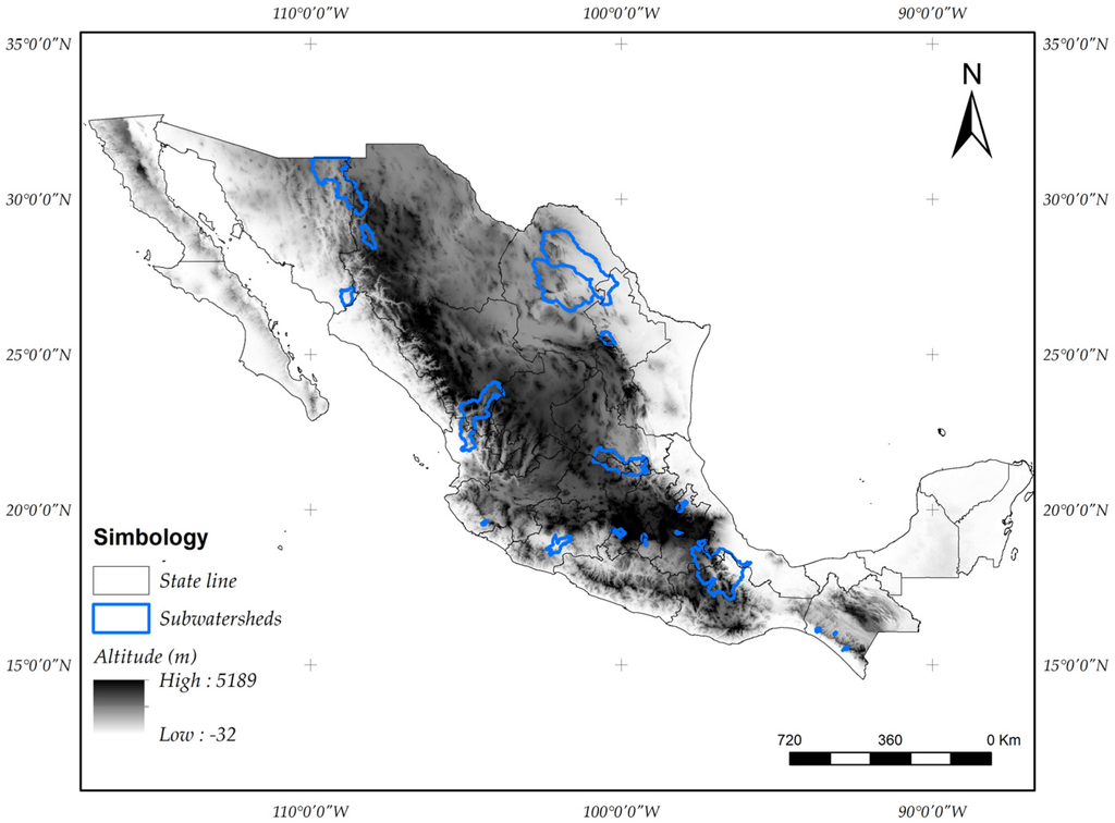
Figure 1.
Locations for the 20 Mexican subwatersheds included in this study.
Hydrological vector data for Mexico were available at the hydrologic region, basin, subwatershed and micro-basin levels according to the Instituto Nacional de Estadística y Geografía (Natonal Institute of Statistics and Geography, INEGI) and the Comisión Nacional para el Conocimiento y Uso de la Biodiversidad (National Commission for Knowledge and Use of Biodiversity, CONABIO) [,]. To convert flow in m3·s−1 to depth in mm·day−1, it is necessary to know the area of the subwatershed that uses the gauging station present as its reference.
The INEGI and CONABIO vectors failed to consider the previous data, which led to conversion overestimations or underestimations. Therefore, subwatersheds were digitized based on their hydrometric station []; the former Hydraulic Resources Secretary [] hydrological bulletins were used as the reference.
Daily precipitation and temperature data were obtained from the National Climate Grid []. The grid consisted of 3147 nodes distributed across the country and separated by 27 km from one another, which have registered daily information on precipitation and minimum and maximum temperature from 1950 to 2013. The information in the climate grid was processed in order to estimate potential evapotranspiration using the Hargreaves [] method.
The data were transformed into an annual scale to enable interpolation through a cubic method. The Python 2.7RM (Python Software Foundation, Amsterdam, The Netherlands) programming language was utilized to obtain the annual average values for each subwatershed and each variable. The soil texture records were obtained from the Food and Agriculture Organization of the United Nations [] Soil Database v 1.2.
2.2. Recession Curves’ Selection
The traditional analytic method for obtaining the master curve required discrimination of n curves per year, which led to a slow and operator-biased extraction process (e.g., Figure 2a). This research proposed to select one annual recession curve per subwatershed, the one with the largest magnitude, which makes the consideration of climate variability among the selected subwatersheds possible (Figure 2b). Recession curves were selected, considering at least three years of hydrometric records. The selected annual curves fit the non-linear model put forward by []:
where Qt is the recession curve for a non-linear reservoir (mm·day−1), Qo is the initial discharge, t is time measured in days and a (RP) and b are the model’s parameters.
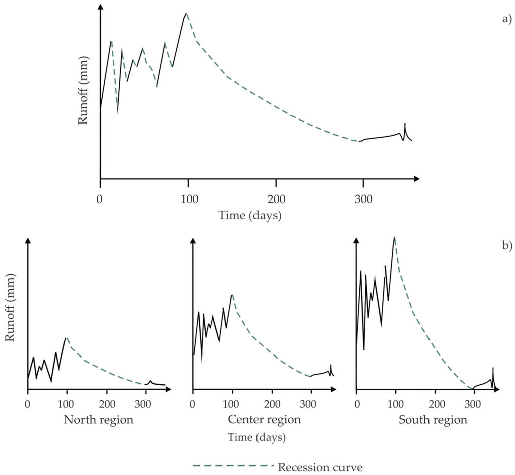
Figure 2.
Recession curves’ selection through the master curve method (dotted line through the year) (a); proposed annual recession curves selection (annual dotted line) (b).
The b exponent value ranges from 0 to 1, corresponding to studies by [,,]. For regionalization purposes, this exponent can be fixed to average conditions b = 0.5, which is a standard value in unconfined aquifers [,].
A contribution of this work, as compared to the aforementioned non-linear models, is that the a (RP) value was fitted and associated with a physiographic characteristic inherent to its subwatershed, adding physical significance to the model.
The Hastie [] criterion (Z) was applied to minimize errors in the objective function and to optimize a:
where is the fitted recession curve, a is the RP and wi is the prediction error.
2.3. Spatial Predictors of the Response of Baseflow and Symmetry in the Process
The area and average slope were analyzed for each subwatershed using topographical variables. The variables obtained from the soil database were percentages for sand, slit and clay. Finally, precipitation due to potential evapotranspiration (NP = ) was normalized. The processed spatial characteristics were related to RP.
The analysis involved the correlation of variables with RP. A threshold of ±0.40 (equivalent to R2 = 0.20) was considered a potentially meaningful correlation []. Potential, exponential and linear functions were calculated for all predictors. The fitting criteria were based on the R2 determination coefficient and the root-mean-square error (RMSE). To avoid multiple methods to evaluate data fit, these two criteria were chosen because they are the most widely used in various hydrological calibrations [,,,].
2.4. Baseflow Separation
The use of a recession curve approach as done by Wittenberg [] required inverting Equation (1), and the baseflow was calculated by combining the recursive filters back and forward. This method assumes that the first and last values of the hydrometric time series represent the baseflow.
This kind of model only displays a statistical array harmonically representing the low frequencies of the surface flow, since it considers neither the intrinsic balances within a subwatershed (water and energy balance) nor the displacement or retention that flow may be affected by (e.g., soil, vegetation and basin shape).
The aim of this study was to find a logical relation between the recession parameter and variables inherent to subwatersheds in order to separate the baseflow. Salas et al. [] found non-linear trends of the recession parameter over the baseflow. Therefore, we proposed to implement a non-linear function in order to estimate the baseflow (BF) in reference to previously-estimated parameters and associate the (α) model dispersion with hydrological characteristics available from the subwatersheds.
The aquifers selected for this analysis were the only ones for which average transmissivity was reported. Table 1 shows hydrogeological values for each subwatershed and its corresponding aquifer.

Table 1.
Subwatershed hydrogeological characteristics [,,,,,,].
3. Results
3.1. Recession Curves
The average recession curves for 21 Mexican subwatersheds were obtained. Table 2 presents calibration results for the curve model. In general, the observed data fit well to the proposed model (R2 > 0.88). The largest magnitude curve was found to be located in the southwest part of the country (San Pedro, Chiapas, hydrometric station Number 30,067), whereas the lowest value was located in a subwatershed in the Mexican northwest (Río Salado-Anahuac, hydrometric station Number 24,038).
Table 2.
Average recession constant fitting summary.
Figure 3 shows the recession pattern spatial trend based on geographical location. It was demonstrated that the RP increases both ways, by decreasing longitude and increasing latitude. The RP values were rescaled to one.
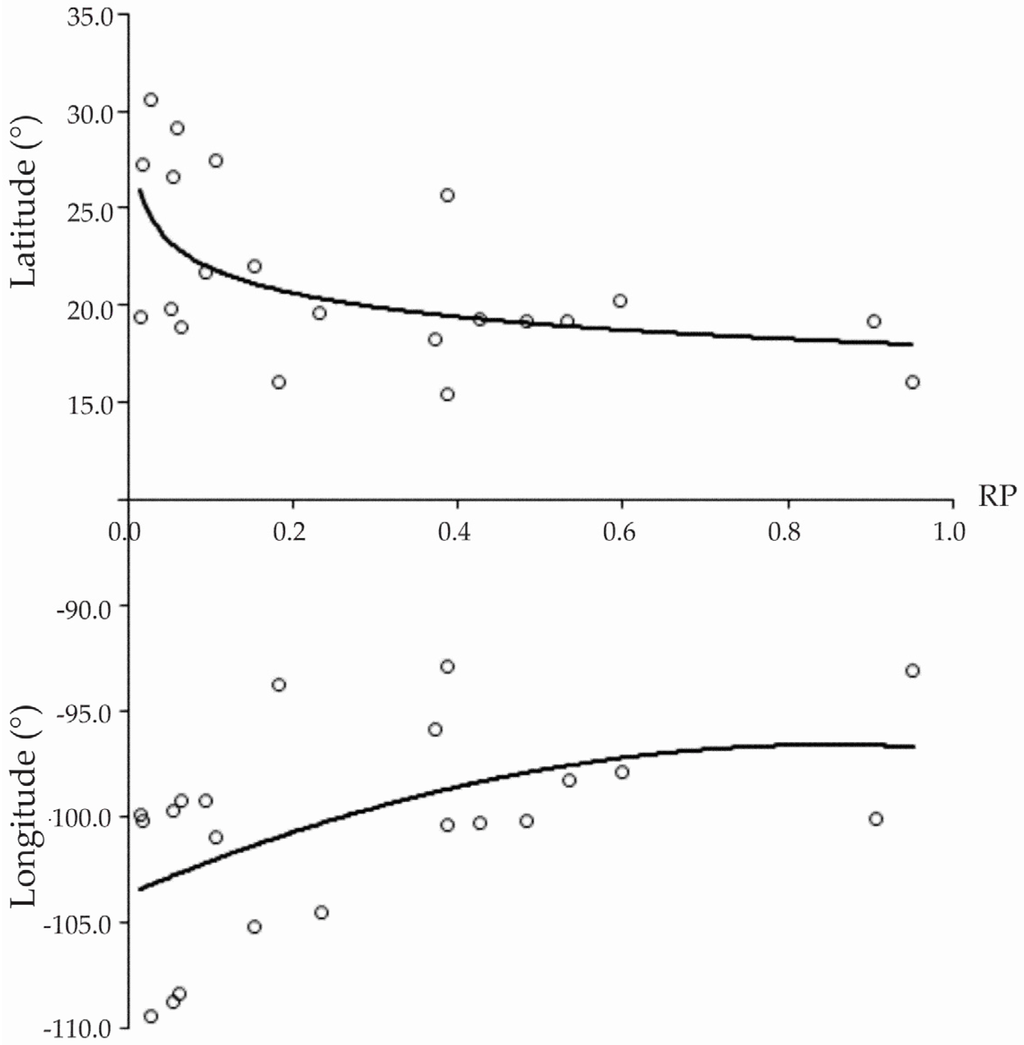
Figure 3.
Relation between the recession parameter (RP) and corresponding longitude and latitude.
3.2. Baseflow Response Spatial Predictors
The dependence of the RP on climate and topographical variables is presented in Figure 4. The relation between the percentages of sand, slit and clay and RP was weak (R2 < 0.14), indicating that the soil variables considered do not affect the fitted parameter. Area and slope were slightly predictive of the parameter (R2 > 0.30); however, these variables were not statistically significant (p > 0.05). With regard to normalized precipitation (NP), a marked non-linear trend with RP was observed (R2 > 0.43), and so, this climate variable was chosen as the principal parameter predictor. The remaining 57% of variance was not explained by this variable. Equation (5) represents this dispersion in the model.
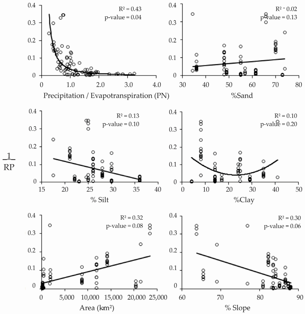
Figure 4.
Relation between recession parameter and landscape and climate variables among subwatersheds.
Figure 5 presents the fitting of the proposed model (Equation (4)), and it shows the variability among subwatersheds (represented by their hydrometric station) and the annual variability of the RP and NP relation for 21 selected subwatersheds. Figure 5a shows the long-term average for RP and NP. Figure 5b presents the corresponding interannual relation. Both relations fit better to the following exponential model:
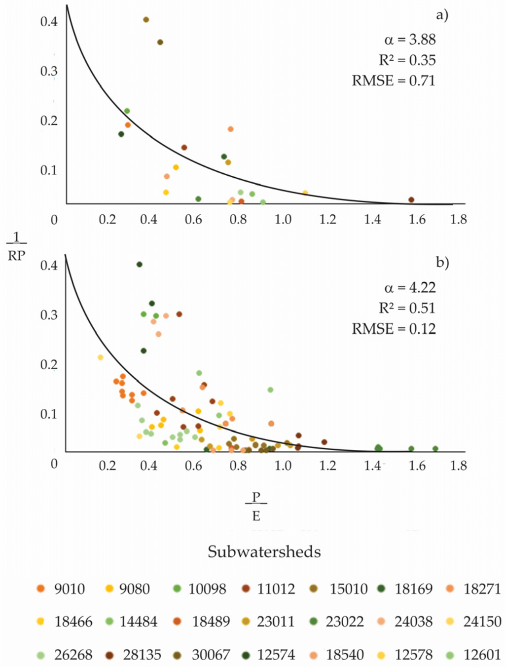
Figure 5.
Subwatershed variability (identified through hydrometric stations) at (a) an interannual scale and (b) subwatershed average long-term variability.
A closer fitting was found for the long-term relation (R2 = 0.51, RMSE = 0.12) as compared to the interannual relation (R2 = 0.35, RMSE = 0.71). The interannual variability showed a higher dispersion than the average long-term variation; even so, this trend and the α fitted parameter were similar in both cases (3.88 vs. 4.22). In this study, the model dispersion (Equation (4)) was associated with the predominant type of rock in each subwatershed and its transmissivity. Transmissivity data were available for only seven subwatersheds.
Figure 6a presents this relation; the storage-discharge relation for subwatersheds with limestone and sandstone surface structures was the most direct (higher RP and transmissivity values), such as the Río Salado and Río Salado de Nadadores subwatersheds (hydrometric station Numbers 24,038 and 24,150). On the other hand, subwatersheds where basalt and crystal rocks are predominant revealed low RP values (e.g., Río Sesecapa, station Number 23,022). At subwatersheds presenting a mixture of permeable and impermeable rock types, the recession curve values were intermediate (e.g., Río Apatlaco, station Number 18,271).
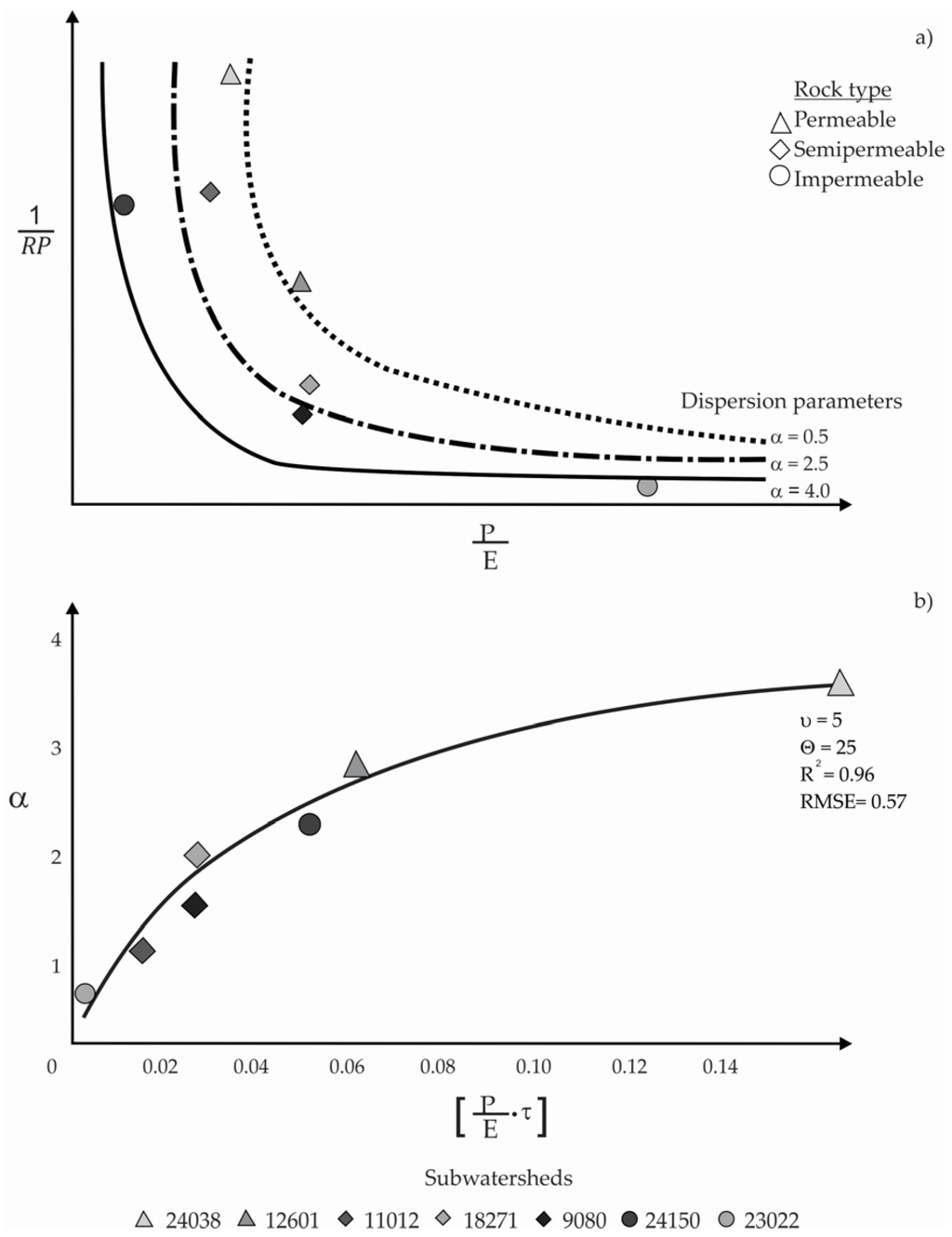
Figure 6.
Subwatershed variability (identified through hydrometric station) and rock type. Relation between the dispersion parameter estimated in the model (a); Equation (4) and the product of and transmissivity (b).
Figure 6b shows the relation between the model’s (Equation (4)) α parameter and the product of by the average transmissivity for each aquifer (τ). A potential model (Equation (5)) was proposed in order to fit this trend (R2 = 0.96, RSME = 0.57). The model depends on two parameters: μ is the maximum reported transmissivity for Mexican aquifers (which could be fixed), and θ is the model’s variation rate in relation to .
3.3. Baseflow Separation
The daily rainfall and streamflow time series were compared to each other. Generally, a more or less one-day lag-time was observed between maximum precipitation events and runoff. We proposed an exponential model, Equation (9), contemplating the recession curve based on in order to separate the baseflow with the following frontier conditions:
Precipitation (P) will always be larger than surface runoff (Qd), which in turn will be larger than baseflow (BF; Equation (6)). The exponential function (Equation (9)) of the model allows BF to come closer to direct flow when is zero (Equation (7)).
The maximum BF events continued after a day with the highest surface runoff and after two days of maximum precipitation (Equation (8)). The proposed generalized model depends on only one parameter estimated in Equation (5):
The BF separation for two subwatersheds with different climate conditions can be observed in Figure 7. The baseflow index (IFB), a proportion of total flow and BF, ranged from 0.39 to 0.36 at the Zanatenco and El Tecolote subwatersheds (hydrometric Stations 23,011 and 15,010).
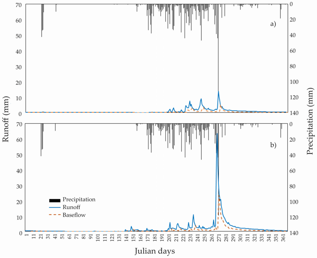
Figure 7.
Separation of baseflow by the generalized baseflow model in the sub-basins: (a) El Tecolote, located in the state of Jalisco, Mexico; and (b) Zanatenco, located in the state of Chiapas, México.
Our results were justified and based on accurate observations of each area. The Zanatenco subwatershed has a precipitation rate higher than 3000 mm per year, whereas the El Tecolote subwatershed presented an annual mean precipitation of 1000 mm. This is the reason why we observed a difference in runoff magnitude in Figure 7.
4. Discussion
Estimating baseflow is a key challenge for hydrological research in Mexico, since there is a lack of large-scale information on subterranean waters dynamics. This study proposed a model based on precise analytical observations of different subwatersheds in the country to estimate baseflow with easily available information and a pragmatic approach.
The model proposed in this research is based on the observation of patterns of invariance and symmetry between sub-basins, rather than empirical adjustments. The response variable (rainfall-evapotranspiration) is hypothesized to be dependent on the availability of water and energy by exponential models, providing a physical explanation to the modeling, besides being feasible to implement, since these variables are readily available at the most basic climatological station.
4.1. Recession Curve
Generally, recession curve analysis is one of the most accurate methods for estimating BF []. Considering the top-down approach by Sivapalan [] and Sivapalan´s proposal of a unified hydrological theory [], this study proposes analyzing different hydrographs per year and subwatershed, which allowed us to obtain recession curves for different climate, topographic and edaphic conditions more efficiently than the master curve method.
Parametrization of recession curves usually implies the use of linear models, where the aquifer’s storage is to be directly proportional to its retention parameter []. As occurred in Wittemberg and Gan and Luo [,], it was observed that recession curves in actual conditions have a concave shape and the estimated parameter steadily increases with decreasing runoff, a strong indication of the non-linearity of the process.
While Thomas et al. [] compared the characteristics of the recession curve between linear and nonlinear models, the results were inconsistent in the linear model, and the authors recommended applying the nonlinear algorithm in sub-basins of New Jersey, USA. Stewart [] showed that the direct flow and base flow in New Zealand watersheds have (non-linear) quadratic characteristics in their relations.
Equation (1) estimates recession curves based on a power law function and invariance properties for scale changes. On various watersheds around the world, authors, such as Wittenberg [] and Wittenberg [], as well as Wittenberg and Sivalapan [], have tested that the b parameter is 0.5 on average. This condition allowed us to only estimate RP and keep b invariant, even with heterogeneous magnitudes of flow in different subwatersheds.
In simple terms, the RP parameter was related to the maximum flow of hydrometric records as observed by Salas et al. []. This revealed information about the humidity and drought of the subwatershed []. The maximum values of RP were found in high latitudes where arid climate prevails, as observed in Figure 3. Although, low RP values were found in humid climates south of Mexico.
Therefore, our result revealed that RP exhibits a trend associated with spatial location. RP increases when angular coordinates decrease. This trend was also found by Sivalapan et al. and Beck et al. [,], who found patterns in the spatial distribution of their fitted parameters allowing them to separate subwatersheds with similar conditions.
4.2. Baseflow Spatial Patterns and Model Parameterization
Different BF response spatial predictors were tested; the NP variable () showed the closest fitting. The importance of using NP lies in potential evapotranspiration (E) varying much less than precipitation (P). Given that the E depends on solar radiation, temperature and latitude, it is a function of energy, and therefore, no major variations are expected through the years. Thus, the E is converted as a scale natural factor for precipitation [].
The climate index commonly used to predict the recession constant is the index of aridity. According to Wang and Wu [], Peña et al. [] and Longombardi and Villani [], it was concluded that the baseflow patterns can be completely modeled with this index, because it considers water and energy limits on its implementation; this type of modeling is feasible by virtue of its physical representation of the phenomenon; and the allure of using a single parameter is that it can be applied in countries where there is not enough data to reproduce a spatially-explicit model [].
Meanwhile, van Dick [] and Lacey and Grayson [] found that the humidity index (HI) was the most closely related variable to the baseflow constant; their studies reported a negative relationship between baseflow and HI. Beck et al. [] found that E, mean temperature, forest coverage and mean subwatershed altitude had the strongest impact on BF. On the other hand, Fan et al. [] stated that precipitation is the main recharge source for aquifers and that baseflow’s response to precipitation depends on the season.
In contrast to Santhi et al. [], this study did not find a significant impact of soil texture on RP on an annual basis (Figure 4). Other studies, such as He et al. [] and Sanchez et al. [], found no relationship between recession constant and soil characteristics, but found a relation with climatic variables. The results matched those of Haberland et al. [], who found that the IFB was related to rainfall and topography, but they did not observe an influence of the properties of soil type or cover in the subwatershed.
Unlike the long-term analysis, higher variability and lower model fitting were found in the interannual analysis. Variability was dependent on the interacting dynamics of energy and water balances [,]. Furthermore, the low model fitting is due to temporary effects, such as temporary storage, as well as macroclimate conditions, which are reflected by means of the estimated model’s parameter in Equation (5). The marked symmetry between RP and NP exhibits climate variability among basins and over years [,], suggesting that the observed trend will carry on in different regions and that applying the same model with the previously-calibrated parameters is feasible [].
The hydrological balance trend depends on climate conditions, and its variability was attributed to landscape conditions []. This study associated the predominant rock type in each subwatershed with its transmissivity, which in turn was associated with the model’s parameter (Equations (9)). Tague and Gran [] assert that subwatershed geology is a primary control in the baseflow-generation process. A more direct storage-discharge relation was found at subwatersheds whose soils were formed by permeable rocks.
According to Price [], permeable or fractured rocks can store large amounts of water, as opposed to crystalline or very compact rocks. At subwatersheds where low-permeability rocks are predominant, RP values were lower. The results agree with Walton []; this author noted that the basins with greater groundwater discharge speed are those with low-permeability rocks. Meanwhile, Sanchez et al. [] found that subwatersheds with basaltic rock presence tended to be drier and to have shorter recession times. These basins are also characterized by a low value of the index of aridity, which can accelerate the recession rate.
4.3. Baseflow Separation
The analyzed subwatersheds were selected by virtue of their minimum anthropogenic disturbances. Therefore, it is feasible to assume that the flow that feeds the outflow during a period of recession corresponds to the BF.
Our research showed that the recession parameter clearly exhibited spatial patterns across subwatersheds []. Subwatersheds within the same climatic conditions (similar values of ) exhibited different RP values, which according to Brooks et al. [] depend on local landscape features, although in our work, it depended on the dominant lithology of each subwatershed. On account of its trend, the recession parameter is assumed to be an aquifer’s recharge rate, which includes the intrinsic properties of each aquifer (hydraulic conductivity, porosity, transmissivity and surface) [].
Analyzing the RP over time, Salas et al. [] observed that the recession curve is the scale parameter modeling the separation of baseflow from direct flow by means of a non-linear function. This observation is similar to that presented by Paz et al. [,]. When analyzing potential functions, they concluded that if parameters match at one common point, it means that the parameters are correlated (fit a linear function). In this case, analytical modeling can be simplified to a single parameter, and setting one a priori value is avoided. This approach will be addressed in future research aimed at making comparable methods of setting b subjectively or estimating it analytically.
The daily time series of rainfall and streamflow were compared. Generally, a more or less one-day lag-time was observed between maximum precipitation events and runoff. According to Caro and Eagleson [], the lag-time is due to an increased hydraulic charge within the aquifer accelerating the stored water exfiltration towards the main currents. The exponential model proposal complies with the principle of BF never being equal to direct flow, due to the ground storage-evapotranspiration interaction, even with no precipitation [].
This research is based on a top-down approach, that is to say, with the information available and hydrological support, it is possible to infer a complex phenomenon, which is commonly analyzed under a reductionist approach []. One example of this is given by Gholami et al. [], who analyzed subterranean water fluctuations using dendrochronology with satisfactory results. These examples challenged the paradigm of always using the same variables in hydrological studies and offered an alternative to apply these conditions in future research.
The proposed BF generalized model requires only precipitation and evapotranspiration variables to estimate baseflow; these variables are readily available across the country, making its operational implementation feasible. The model has one additional distinct advantage: the maximum Qb events correspond to the recession curve initial value. According to Aksoy and Wittemberg [], the aforementioned feature involves an aquifer’s recharge-storage-discharge interactions. The advantages of applying this type of model are the possibility of interpreting parameters by their association with observable physical features and operative parsimony [].
The analysis presented in this paper separated the BF for 21 Mexican subwatersheds. Furthermore, a coherent digitalization for each acquisition area was obtained, i.e., the measuring station was deemed the starting and ending point for determining each subwatershed surface, which contrasts with current basin cartographic products in the country.
The climate grid contains information under quality control standards, which allows for certainty regarding input data. Furthermore, the basin-to-basin analysis of annual recession curves showed the intrannual interaction within those basins due to climate variability.
Although information on vegetation and groundwater levels is not available operationally in the country, this study was directed towards the discovery of patterns in the obtainable data and the formulation of hypotheses concerning subwatershed interactions, aiming to avoid the redundancy of using observations to calibrate a priori constructed models [].
5. Conclusions
The results of this study demonstrate that baseflow (BF) can be separated from direct flow by using a single-parameter non-linear model. The higher variability and low model fitting of our proposed model was related to subwatershed geology and climate variables. This allowed us to use variables that are easily available in the country. It was feasible to calibrate the non-linear model using only the longer duration recession curve, unlike the traditional approach using the master curve.
The recession curve maintains a symmetric trend over years and within measured subwatersheds located in protected natural areas with diverse landscapes and climate conditions in Mexico. The BF generalized model is a result of accurate observations from different geographic regions in the country, and so, it can be utilized for separating BF in non-measured basins. Our ensuing research considers analyzing the interaction of BF with available ground humidity for short time scales.
Despite the limited information, the generalized BF model may represent a baseline for the generation of alternative modeling approaches. Such an accomplishment should include functional elements that explore the baseflow behavior based on multiple spatial and temporal scales. In order to improve the calibration model, we recommend incorporating local variables (e.g., canopy, soil moisture, groundwater levels), and we also suggest including subwatersheds affected by anthropogenic activity, so as to analyze flow changes ascribable to climate oscillation or human influence.
Acknowledgments
The authors would like to thank the CONACyT for financing the doctoral studies. This work has been partially support by Colegio de Postgraduados, Secretaria de Agricultura, Ganaderia, Desarrollo Rural, Pesca y Alimentación (SAGARPA).
Author Contributions
The research presented was developed in collaboration of all of the authors. Salas-Aguilar and Paz had the original idea for the study. Macedo-Cruz, Palacios, Ortiz and Quevedo conducted the research methods. All authors discussed the structure and commented on the manuscript at all stages.
Conflicts of Interest
The authors declare no conflict of interest.
References
- Campolo, M.; Soldati, A.; Andreussi, P. Forecasting river flow rate during low-flow periods using neural networks. Water Resour. Res. 1999, 35, 3547–3552. [Google Scholar] [CrossRef]
- Van Dijk, A.I. Climate and terrain factors explaining streamflow response and recession in Australian catchments. Hydrol. Earth Syst. Sci. 2010, 14, 159–169. [Google Scholar] [CrossRef]
- Beck, H.L.; van Dijt, A.; Miralles, D.G.; McVicar, T.R.; Schellekens, J. Global patterns in baseflow index and recession based on streamflow observations from 3394 catchments. Water Resour. Res. 2013, 49, 7843–7863. [Google Scholar] [CrossRef]
- Budyko, M.I. Climate and Life; Academics: New York, NY, USA, 1974. [Google Scholar]
- Fu, B.P. On the calculation of the evaporation from land surface. Sci. Atmos. 1981, 1, 23–31. (In Chinese) [Google Scholar]
- Zhang, L.; Dawes, W.R.; Walker, G.R. Response of mean annual evapotranspiration to vegetation changes at catchment scale. Water Resour. Res. 2001, 3, 701–708. [Google Scholar] [CrossRef]
- Gerrits, A.M.J.; Savenije, H.H.G.; Veling, E.J.M.; Pfister, L. Analytical derivation of the Budyko curve based on rainfall characteristics and a simple evaporation model. Water Resour. Res. 2009, 45. [Google Scholar] [CrossRef]
- Troch, P.A.; Carrillo, G.; Sivapalan, M.; Wagener, T.; Sawlez, K. Climate-vegetation-soil interactions and long-term hydrologic partitioning: Signatures of catchment co-evolution. Hydrol. Earth Syst. Sci. 2013, 17, 2209–2217. [Google Scholar] [CrossRef]
- Wang, L.; Wu, L. Similarity of climate control on baseflow and perennial stream density in the Budyko framework. Hydrol. Earth Syst. Sci. 2013, 17, 315–324. [Google Scholar] [CrossRef]
- Santhi, C.; Allen, P.; Muttiah, M.R.S.; Arnold, J.G.; Tuppad, P. Regional estimation of base flow for the conterminous United States by hydrologic landscape regions. J. Hydrol. 2008, 351, 139–153. [Google Scholar] [CrossRef]
- Longobardi, A.; Villani, P. Baseflow index regionalization analysis in a mediterranean area and data scarcity context: Role of the catchment permeability index. J. Hydrol. 2008, 355, 63–75. [Google Scholar] [CrossRef]
- Wang, T.; Istanbulluoglu, E.; Lenters, J.; Scott, D. On the role of groundwater and soil texture in the regional water balance: An investigation of Nebraska Sand Hills. Water Resour. Res. 2009, 45. [Google Scholar] [CrossRef]
- Istanbulluoglu, E.; Tiejun, W.; Wright, O.; Lenters, J.D. Interpretation of hydrologic trends from a water balance perspective: The role of groundwater storage in the Budyko’s hypothesis. Water Resour. Res. 2012, 48. [Google Scholar] [CrossRef]
- Sivapalan, M. Pattern, process and function: Elements of a unified theory of hydrology at the catchment scale. In Encyclopedia of Hydrological Sciences; Jhon Wiley Ltd.: West Sussex, UK, 2005; Chapter 13; pp. 193–219. [Google Scholar]
- Ponce, V.M.; Shetty, A.V. A conceptual model of catchment water balance: Formulation and calibration. J. Hydrol. 1995, 173, 27–40. [Google Scholar] [CrossRef]
- Sivapalan, M.; Yaeger, M.A.; Ciaran, H.J.; Xiangyu, X.; Troch, P.A. Functional model of wáter balance variablity at the catchment scale: 1. Evidence of hydrologic similiraty and space-time symmetry. Water Resour. Res. 2011, 47. [Google Scholar] [CrossRef]
- Harman, C.J.; Troch, P.A.; Sivapalan, M. Functional model of water balance variability at the catchment scale: 2. Elasticity of fast and slow runoff components to precipitation change in the continental United States. Water Resour. Res. 2011, 47. [Google Scholar] [CrossRef]
- Tallaksen, L. A review of baseflow recession analisys. J. Hydrol. 1995, 165, 349–370. [Google Scholar] [CrossRef]
- Eckhardt, K. How to construct recursive digital filters for Baseflow separation. Hydrol. Process. 2005, 19, 507–515. [Google Scholar] [CrossRef]
- Huyck, A.; Pauwels, V.; Vershoest, N. A baseflow separation algorithm based on the linearized boussinesq equation for complex hillslopes. Water Resour. Res. 2005, 41. [Google Scholar] [CrossRef]
- He, S.; Li, S.; Xie, R.; Lu, J. Baseflow separation based on a metereology corrected nonlinear algorithm in typical rainy agricultural watershed. J. Hydrol. 2016, 535, 418–428. [Google Scholar] [CrossRef]
- Paz, F.; Odi, M.; Cano, A.; Bolaños, M.; Zarco, A. Equivalencia ambiental en la productividad de la vegetación. Agrociencia 1999, 43, 635–648. (In Spanish) [Google Scholar]
- Banco Nacional de Datos de Aguas Superficiales, 2011. Consulta de Datos Hidrométricos, de Presas y Sedimentos. Comisión Nacional del Agua: México. Available online: www.conagua.gob.mx/CONAGUA07/contenido/documentos/portada%20bandas.htm (accessed on 25 January 2015).
- García, E. Climas, 1:4000 000. IV.4.10 (A). Atlas Nacional de México Vol. II; Instituto de Geografía, UNAM.: Ciudad de México, México, 1990. (In Spanish) [Google Scholar]
- Instituto Nacional de Estadística, Geografía e Informática (INEGI). Red Hidrográfica Escala 1:50,000 Edición 2.0. Available online: http://www.inegi.org.mx/geo/contenidos/topografia/regiones_hidrograficas.aspx (accessed on 16 Junuary 2016).
- Comisión Nacional para el Conocimiento y Uso de la Biodiversidad (CONABIO). Subcuencas Hidrológicas. Available online: http://www.conabio.gob.mx/informacion/metadata/gis/subcu1mgw.xml?_httpcache=yes&_xsl=/db/metadata/xsl/fgdc_html.xsl&_indent=no (accessed on 15 January 2015).
- Programa Mexicano del Carbono (PMC). Digitalización de Subcuencas Escala 1,50000; Programa Mexicano del Carbono: Texcoco, Estado de México, México, 2014. [Google Scholar]
- Secretaria de Recursos Hidráulicos (SRH). Boletines Hidrológicos; Gerencia de Aguas Superficiales: Ciudad de México, México, 1970.
- Programa Mexicano del Carbono (PMC). Malla Climática Nacional; Programa Mexicano del Carbono (PMC): Texcoco, México, 2015. (In Spanish) [Google Scholar]
- Hargreaves, G.H.; Samani, Z.A. Reference crop evapotranspiration from temperature. Appl. Eng. Agric. 1985, 1, 96–99. [Google Scholar] [CrossRef]
- Food and Agriculture Organization of the United Nations (FAO). Harmonized Database of Soil. Available online: http://www.fao.org/soils-portal/levantamiento-de-suelos/mapas-historicos-de-suelos-y-bases-de-datos/base-de-datos-armonizada-de-los-suelos-del-mundo-v12/es/ (accessed on 10 January 2015).
- Wittenberg, H. Nonlinear analysis of flow recession curves. IAHS Publ. 1994, 221, 61–67. [Google Scholar]
- Wittenberg, H. Baseflow recession and recharge as nonlinear storage processes. Hydrol. Process. 1999, 13, 715–726. [Google Scholar]
- Aksoy, H.; Wittenberg, H. Nonlinear baseflow recession analysis in watersheds with intermittent streamflow. Hydrol. Sci. J. 2011, 56, 226–237. [Google Scholar] [CrossRef]
- Gan, R.; Luo, Y. Using the nonlinear aquifer storage-discharge relationship to simulate the baseflow of glacir—And snowmelt-dominated basins in northwest China. Hydrol. Earth Syst. Sci. 2013, 17, 3577–3586. [Google Scholar] [CrossRef]
- Aksoy, H.; Wittenberg, H. Baseflow Recession Analysis for Flood-Prone Black Sea Watersheds in Turkey. Clean Air Soil Water 2015, 42, 1–10. [Google Scholar] [CrossRef]
- Hastie, T.; Tibshirani, R.; Friedman, J. The Elements of Statistical Learning: Prediction, Inference and Data Mining, 2nd ed.; Springer Verlag: New York, NY, USA, 2009. [Google Scholar]
- Salas, A.V.; Paz, F.; Macedo, C.; Ortiz, C.; Palacios, E. Modelación no lineal del flujo base en tres subcuencas de México. Terra Latinoam. 2015, 33, 285–297. (In Spanish) [Google Scholar]
- Comisión Nacional del Agua (CONAGUA). Determinación de la Disponibilidad de Agua Subterránea en el Acuífero 0859; Subdirección General Técnica de Aguas Subterraneas: Madera, México, 2013. [Google Scholar]
- Comisión Nacional del Agua (CONAGUA). Actualización de la Disponibilidad de Agua Subterránea en el Acuífero 1802; Subdirección General Técnica de Aguas Subterraneas: San Pedro Tuxpan, México, 2009. [Google Scholar]
- Comisión Nacional del Agua (CONAGUA). Actualización de la Disponibilidad de Agua Subterránea En el Acuífero 1502; Subdirección General Técnica de Aguas Subterraneas: Ixtlahuaca-Atlacomulco, México, 2009. [Google Scholar]
- Comisión Nacional del Agua (CONAGUA). Determinación de la Disponibilidad de Agua en el Acuífero 1701; Subdirección General Técnica de Aguas Subterraneas: Cuernavaca, México, 2013. [Google Scholar]
- Comisión Nacional del Agua (CONAGUA). Actualización de la Disponibilidad Media Anual de Agua Subterránea Acuífero 0711; Subdirección General técnica de Aguas Subterraneas: Arriaga-Pijijiapan, México, 2009. [Google Scholar]
- Comisión Nacional del Agua (CONAGUA). Actualización de la Disponibilidad de Agua Subterránea en el Acuífero 0512; Subdirección General Técnica de Aguas Subterraneas: Región Carbonífera, México, 2013. [Google Scholar]
- Comisión Nacional del Agua (CONAGUA). Actualización de la Disponibilidad de Agua Subterránea en el Acuífero 0507; Subdirección General Técnica de Aguas Subterraneas: Monclova, México, 2013. [Google Scholar]
- Sivapalan, M. Prediction of ungauged basin: A gran challenge for theoretical hydrology. Hydrol. Process. 2003, 17, 3163–3170. [Google Scholar] [CrossRef]
- Pedersen, T.J.; Peters, J.C.; Helweg, O. Hydrographs by single linear reservoir model. J. Hydraul. Div. ASCE 1980, 106, 837–852. [Google Scholar]
- Thomas, B.; Voegel, R.; Famiglietti, J. Objetive hydrograph Baseflow recession analysis. J. Hydrol. 2015, 525, 102–112. [Google Scholar] [CrossRef]
- Stewart, M.K. Promising new Baseflow separation and recession analysis methods applied to streamflow at Glendhu Catchment, New Zealand. Hydrol. Earth Syst. Sci. 2015, 19, 2587–2603. [Google Scholar] [CrossRef]
- Wittenberg, H. Effects of season and man-made changes on baseflow and flow recession: Case studies. Hydrol. Process. 2003, 17, 2113–2123. [Google Scholar] [CrossRef]
- Wittenberg, H.; Sivapalan, M. Watershed groundwater balance estimation using streamflow recession analysis and baseflow separation. J. Hydrol. 2003, 219, 20–33. [Google Scholar] [CrossRef]
- Dralle, D.; Karst, N.; Thompson, S. a, b careful: The challenge of scale invariance for comparative analyses in power law models of the streamflow recession. Geophys. Res. Lett. 2015, 42, 9285–9293. [Google Scholar] [CrossRef]
- Carmona, A.M.; Sivalapan, M.; Yaeger, M.A.; Poveda, G. Regional patterns variability of catchment water balances across the continental U.S.: A Budyko framework. Water Resour. Res. 2014, 50. [Google Scholar] [CrossRef]
- Peña-Arancibia, J.L.; van Dijk, A.I.J.M.; Mulligan, M.; Bruijnzeel, L.A. The role of climatic and terrain attributes in estimating baseflow recession in tropical catchments. Hydrol. Earth Syst. Sci. 2010, 14, 2193–2205. [Google Scholar] [CrossRef]
- Lacey, G.; Grayson, R. Relating baseflow to catchment properties in south-eastern Australia. J. Hydrol. 1998, 204, 231–250. [Google Scholar] [CrossRef]
- Fan, Y.; Chen, Y.; Li, W. Increasing precipitation and baseflow in Aksu River since 1950s. Quat. Int. 2014, 336, 26–34. [Google Scholar] [CrossRef]
- Sanchez, R.; Brooks, E.; Elliot, W.; Gazel, E.; Boll, J. Baseflow recession analysis in the inland Pacific Northwest of the United States. Hydrogeol. J. 2015, 23, 287–303. [Google Scholar] [CrossRef]
- Haberlandt, U.; Klocking, B.; Krysanova, V.; Becker, A. Regionalisation of the baseflow indexfrom dynamically simulated flow components—A case study in the Elbe River Basin. J. Hydrol. 2001, 248, 35–53. [Google Scholar] [CrossRef]
- Yang, D.; Shao, W.; Yeh, P.; Yang, H.; Kanae, S.; Oki, T. Impact of vegetation coverage on regional water balance in the nonhumid regions of China. Water Resour. Res. 2009, 45, 1–13. [Google Scholar] [CrossRef]
- Tague, C.; Grant, G.E. A geological framework for interpreting the low-flow regimes of Cascade streams, Willamette River Basin, Oregon. Water Resour. Res. 2004, 40, 150–178. [Google Scholar] [CrossRef]
- Price, K. Effects of watershed topography, soils, land use and climate on baseflow hydrology in humid regions: A review. Prog. Phys. Geogr. 2011, 4, 465–492. [Google Scholar] [CrossRef]
- Walton, W.C. Ground Water Recharge and Runoff in Illinois; Report of Investigation; Illinois State Water Survey; State Water Survey Division: Champaign, IL, USA, 1965; p. 55. [Google Scholar]
- Voepel, H.; Rudell, B.; Shumer, R.; Troch, P.; Brooks, P.; Neal, A.; Durcik, M.; Sivapalan, M. Quantifying the role climate and landscape characteristics on hydrologic partitioning and vegetation response. Water Resour. Res. 2011, 47, 1–13. [Google Scholar] [CrossRef]
- Brooks, P.D.; Troch, P.A.; Durcik, M.; Gallo, E.L.; Moravec, B.G.; Schlegel, M.E.; Carlson, M. Quantifying regional-scale ecosystem response to changes in precipitation: Not all rain is created equal. Water Resour. Res. 2011, 47. [Google Scholar] [CrossRef]
- Paz, F.; Odi, M.; Cano, A.; Lopez, E.; Bolaños, M.; Zarco, A.; Palacios, E. Elementos para el desarrollo de una hidrologia operacional con sensors remotos: Mezcla suelo-vegetación. Tecnol. Cienc. Agua 2009, 24, 69–80. [Google Scholar]
- Caro, R.; Eagleson, P.S. Estimating aquifer recharge due to rainfall. J. Hydrol. 1981, 53, 185–211. [Google Scholar] [CrossRef]
- Bart, R.; Hope, A. Inter-seasonal variability in base flow recession rates: The role of aquifer antecedent storage in central California watersheds. J. Hydrol. 2014, 519, 205–213. [Google Scholar] [CrossRef]
- Gholami, V.; Chau, K.; Fadaee, F.; Torkaman, J.; Ghaffari, A. Modeling of groundwater level fluctuations using dendrochronology in alluvial aquifers. J. Hydrol. 2015, 529, 1060–1069. [Google Scholar] [CrossRef]
- Archontoulis, S.; Miguez, F. Nonlinear regression models and applications in agricultural research. Agron. J. 2015, 105, 1–13. [Google Scholar] [CrossRef]
© 2016 by the authors; licensee MDPI, Basel, Switzerland. This article is an open access article distributed under the terms and conditions of the Creative Commons by Attribution (CC-BY) license (http://creativecommons.org/licenses/by/4.0/).