Article

Historical Trends in Mean and Extreme Runoff and Streamflow Based on Observations and Climate Models

Civil Engineering Department and NOAA-CREST, The City College of New York, City University of New York, New York, NY 10031, USA
*
Author to whom correspondence should be addressed.
Water 2016, 8(5), 189; https://doi.org/10.3390/w8050189
Submission received: 20 December 2015 / Revised: 27 April 2016 / Accepted: 28 April 2016 / Published: 7 May 2016

Abstract

:
To understand changes in global mean and extreme streamflow volumes over recent decades, we statistically analyzed runoff and streamflow simulated by the WBM-plus hydrological model using either observational-based meteorological inputs from WATCH Forcing Data (WFD), or bias-corrected inputs from five global climate models (GCMs) provided by the Inter-Sectoral Impact Model Intercomparison Project (ISI-MIP). Results show that the bias-corrected GCM inputs yield very good agreement with the observation-based inputs in average magnitude of runoff and streamflow. On global average, the observation-based simulated mean runoff and streamflow both decreased about 1.3% from 1971 to 2001. However, GCM-based simulations yield increasing trends over that period, with an inter-model global average of 1% for mean runoff and 0.9% for mean streamflow. In the GCM-based simulations, relative changes in extreme runoff and extreme streamflow (annual maximum daily values and annual-maximum seven-day streamflow) are slightly greater than those of mean runoff and streamflow, in terms of global and continental averages. Observation-based simulations show increasing trend in mean runoff and streamflow for about one-half of the land areas and decreasing trend for the other half. However, mean and extreme runoff and streamflow based on the GCMs show increasing trend for approximately two-thirds of the global land area and decreasing trend for the other one-third. Further work is needed to understand why GCM simulations appear to indicate trends in streamflow that are more positive than those suggested by climate observations, even where, as in ISI-MIP, bias correction has been applied so that their streamflow climatology is realistic.

1. Introduction

Anthropogenic changes in global climate and alteration of Earth’s hydrological cycle [1,2,3] have resulted in increased heavy precipitation with consequent increased surface runoff and flooding risk [4,5], which is likely to worsen in the future [6]. Climate change is expected to change the pattern, frequency and intensity of precipitation and result in increased intensity and frequency of floods and droughts, with damaging effects on environment and society [5,6,7,8,9,10,11,12].
As a result of greenhouse gas (GHG) build-up in the atmosphere, global mean near-surface temperature shows an increasing trend since the beginning of the 20th century [11,13,14]. The Fifth Assessment Report of Inter-Governmental Panel on Climate Change (IPCC) indicates that global land and ocean near-surface air temperature has increased by approximately 0.78 °C, over the 20th century, with greater trend slope in recent decades [15]. As a result of global warming, global climate models (GCMs) and satellite observations both indicate that atmospheric water vapor content has increased at a rate of approximately 7% per K warming [1,2,3,16], as expected from the Clausius-Clapeyron equation under stable relative humidity [2,17]. Increasing availability of moisture in the atmosphere can be expected to result in increased intensity of extreme precipitation [1,5,7,8,18], with proportionally greater impact than for mean precipitation [17,19]. An increase in frequency and intensity of extreme precipitation has already been identified in observations [9,11,20,21,22,23] as well as in simulations of GCMs [22,24,25,26], and GCMs also indicate that further increases in extreme precipitation would be expected over the next decades [8,17,24,25,27]. In terms of mean precipitation, some studies suggest that moist regions become wetter and dry regions drier [3,18,28,29], while some recent studies challenge this concept [30].
Increased risk of flooding due to anthropogenic climate change has also been stressed often in the literature. However, there are few studies of trends in flooding at global or continental scales [6,31,32,33,34], as most studies have been limited to basin or country scales [35,36,37,38]. A study of global runoff projections from three GCMs for the last decades of the 21st century shows, with large variation among the models, strong increase at high latitudes and significant decrease at some mid-latitude regions [39]. Analysis of future projections of runoff from 23 GCMs from the Fourth Assessment Report (AR4) of IPCC also revealed projected increases in northern regions and decreases in some parts of the mid-latitudes [40].
Simulations of historical precipitation and other climate variables by GCMs generally show systematic deviations from observations (biases). This results from various causes, such as model imperfection in atmospheric physics and parameterization, and can alter the results of climate change impact studies [5,41,42,43]. Such errors and deviations affect the reliability of future projections of GCMs and make their outputs inapplicable as direct input to global hydrological models for climate change impact studies [39,44]. Bias correction methods are often adopted as a solution for this issue, in which the mean value is adjusted by applying a temporally constant offset or correction coefficient to the data. Although such adjustment affects the mean value, it is supposed to preserve the trend in time series of the data since the applied corrections are time independent [41]. Bias correction thus preserves differences of trends between GCMs and/or with respect to various emissions scenarios [41,44]. The impact of bias correction on trends in climate extremes remains to be further studied [41,43].
The Inter-Sectoral Impact Model Intercomparison Project (ISI-MIP) [45] presents bias-corrected meteorological data and hydrological model outputs such as runoff and streamflow, which provides the opportunity to investigate streamflow under climate change considering the biases and uncertainties [6]. An initial assessment of the changes in the 30-y return level of five-day average peak flows (Q30) in data provided by ISI-MIP from 1971 to 2000 shows an increase in the magnitude and frequency of the 30-y return level of river flow at roughly two-thirds of the global land areas, with decreases mostly occurring in snowfall-dominated regions. Analysis of future projections reveals that, Central and Eastern Siberia and parts of Southeast Asia, show projected increases in Q30, while Northern and Eastern Europe and parts of Northwestern North America show a decrease [6]. Another multi-model study of ISI-MIP projected changes in streamflow for the 21st century shows strong increases in northern high latitudes, Eastern Africa and India, and deceases in Southern Europe, the Mediterranean, and large parts of North and South America [46], similar to some other studies [39,40]. However, the reliability of the ISI-MIP streamflow simulations, especially for extreme events, remains to be investigated [41].
Change in streamflow also has implications for available water resources. Current and future impact of climate change on available water resources has been widely noted by earlier studies [15,47,48,49,50]. Climate change is likely to increase water stress in the regions that experience decreased precipitation and runoff. It may even increase stress in regions with increased average precipitation and runoff, due to change in the precipitation pattern, where the excess water comes in more intense bursts and in the wet seasons and not the dry seasons [49,50]. One of the main obstacles to study streamflow trends is that streamflow data are not publicly available for most land areas [51]. Global scale runoff and streamflow trends can be studied through the analysis of the outputs of global hydrological models. Given observed or simulated meteorological values such as precipitation, temperature and relative humidity, a hydrological model can generate corresponding streamflow and/or runoff outputs. Utilizing a global hydrological model, particularly if it can be validated against a large number of past streamflow observations, provides us with a robust tool to study the historical and future changes in streamflow, and consequently fresh-water resources, based on either observed or modeled climate changes.
In the present study, runoff and streamflow generated by the WBM-plus global hydrological model [52], which will simply be called WBM in the remainder of the paper, based on the observation-based meteorological inputs from WATCH Forcing Data (WFD) [53] are statistically analyzed at global and continental scales, for the time period of 1971–2001. Runoff and streamflow generated by the WBM model based on bias-corrected outputs of GCMs, provided by the ISI-MIP, are also analyzed to compare the modeled and observational meteorology based trends in runoff and streamflow for the time period of 1971–2001, at global and continental scales. The WFD datasets are used in ISI-MIP project for bias correction of GCMs [41] and provide a fair basis for comparison of GCMs with observation-based simulations.
The analyses presented in this paper are therefore as follows. The WBM model performance in simulation of streamflow is first evaluated based on observation-based forcings and observational streamflow data for the coterminous United States (US). Annual-mean daily runoff and streamflow for the WFD and ISI-MIP data are then analyzed to study the changes in mean flow based on GCMs versus observations. Annual-maximum daily runoff and streamflow are also analyzed with the GCM outputs to study the changes in extreme flows and in comparison with changes in mean flow. Trends in annual-maximum seven-day streamflow are additionally analyzed to study the changes in lengthier extreme flows in comparison with shorter one-day extremes.

2. Materials and Methods

We study changes in mean and extreme runoff and streamflow. Mean runoff is defined as the annual-mean daily runoff, which is the annual average of daily runoff values. Extreme runoff is defined as the annual-maximum daily runoff, in which the maximum daily runoff is selected for each year. Similar to runoff, mean streamflow is defined as the annual-mean daily streamflow, in which the daily flow rates are averaged for each year. Extreme streamflow is defined as the annual-maximum daily streamflow, in which the maximum daily flow rate value is selected for each year. Annual-maximum 7-day streamflow is also calculated, for which average flow rate is calculated for each consecutive 7-day period (moving average) and then the maximum value is selected for each year.
ISI-MIP presents bias-corrected daily meteorological fields, at a uniform 0.5 degree spatial resolution, from 5 selected GCMs from the fifth phase of the Coupled Model Intercomparison Project (CMIP5), which provides the opportunity to investigate the impacts of climate change from a range of GCMs on water resource system design after bias correction [6]. The first fast-track phase of the ISI-MIP project presents outputs from the following 5 GCMs: GFDL-ESM2M, HadGEM2-ES, IPSL-CM5A-LR, MIROC-ESM-CHEM and NorESM1-M [45].
One of the main obstacles in study of streamflow is that streamflow data is not publicly available for most land areas [51]. Runoff and streamflow trends in global scale can be studied through the analysis of the outputs of global hydrological models. ISI-MIP also provides runoff and streamflow simulations, which have been simulated by various global hydrological models based on bias-corrected outputs of the 5 CMIP5 global climate models. For the purposes of the present study, the runoff and streamflow simulations of the WBM hydrological model based on bias-corrected GCM inputs are obtained from the ISI-MIP.
ISI-MIP project uses the WATCH Forcing Data (WFD) [53] observation-based dataset for bias correction. Hence, for sake of fair comparison, runoff and streamflow generated by the WBM model based on WFD observation-based inputs are studied here as the observational-based runoff and streamflow data sets. The Water Balance Model (WBM), maintained at the City College of the City University of New York, is a macro-scale hydrological model that simulates water exchange between the land surface and the atmosphere as well as water transport along a prescribed river network. The model runs on spatial resolutions as high as of 0.1 degree and daily temporal resolution. The model can account for human activities such as irrigation water abstraction and reservoir operation [52]. The runoff and streamflow data simulated by the WBM model using WFD forcing are also at 0.5 degree spatial resolution and comparable with those of the ISI-MIP project.
Tests for the determination of significant trends in climatologic time series can be classified as parametric or non-parametric. Parametric trend tests are derived on the assumption of independence and normal distribution in the data, while non-parametric trend tests require only that the data be independent. The trend slope (b) obtained from the linear regression method, which assumes that the data variability follows a normal distribution, is utilized for parametric trend strength analysis and comparison of the datasets. The relative change in runoff (R) and streamflow (Q) is defined as the trend slope divided by the average value of the grid cell (b/R and b/Q, respectively). The Z-score (Z) obtained from the Mann-Kendall test (Appendix A) [54,55] and Qmed from the Sen’s slope estimator (Appendix B) [56] are also applied in order to confirm the results of linear regression using non-parametric trend detection approaches. It should be noted that Qmed denotes an index calculated in Sen’s slope estimator method (Appendix B) for any time series (such as runoff and streamflow), and is not related to the connotation of Q as discharge or streamflow.
Dry grid cells with average discharge of less than 0.01 mm/day [57] for the period of 1971–2001 based on WFD observation-based data, as well as Greenland and Antarctica, are excluded from the calculations. The remaining grid cells cover about 76% of global land area. The trend tests are applied for each grid cell’s runoff and streamflow time series. The obtained values are also averaged globally as well as by continent in order to present the general trend of runoff and streamflow in different regions. The averaging is weighted by grid cell area, meaning that the larger cells in tropics have higher impact on the average than the smaller cells in high latitudes. The continents studied comprise Africa, Asia, Europe, North America, South America and Oceania. The subcontinent of India has results shown separately and is also included in Asia.

3. Results and Discussion

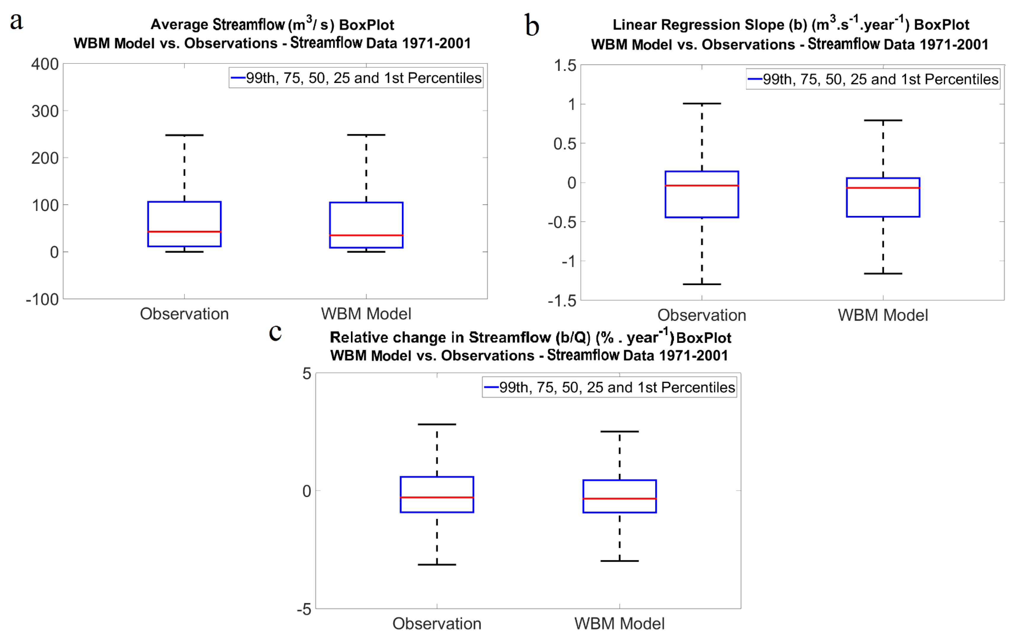
3.1. Hydrological Model (WBM) Performance Evaluation

The performance of the WBM model in simulation of river discharge based on the WFD observation-based meteorological inputs is evaluated. The Coterminous US, which is generally considered to have more complete and reliable observational meteorological data, compared to most other regions, is chosen as the evaluation area. Limiting the performance evaluation of the hydrological model to a region with more reliable data will help in constraining the accuracy of the results mostly to the performance of the model rather than inaccuracy of the input data. Figure 1 depicts the maps of average streamflow and its trend from 1971 to 2001 for the US region, simulated by WBM and compared to USGS station observations. Due to high variability of the streamflow values at different locations, the streamflow magnitude maps are plotted in logarithmic scale. Figure 1c illustrates that the eastern and north-western parts of the US have had a decreasing trend in streamflow for 1971–2001, while the central parts experienced increases in flow.
Figure 2 shows the magnitude and change in streamflow of the United States from 1971 to 2001 in the model outputs as well as observations. It should be noted that the observational streamflow data are station-based, and show the discharge at the point of measurement, whereas the modeled data are grid-based and show the discharge rate per grid cell. Hence, the magnitude of discharge may not be comparable between observations and models. However, the relative change in the discharge, which is the ration of the slope of change in discharge and the mean magnitude of discharge (b/Q), has units of % per year and is more comparable. As seen in Figure 2, as well as Table 1, the boxplot of relative change in discharge (b/Q) for the model results show a good agreement with the observational results in terms of general distribution of values at different percentiles (Figure 2c), which indicates that the WBM model simulates the relative change in river discharge with suitable accuracy.

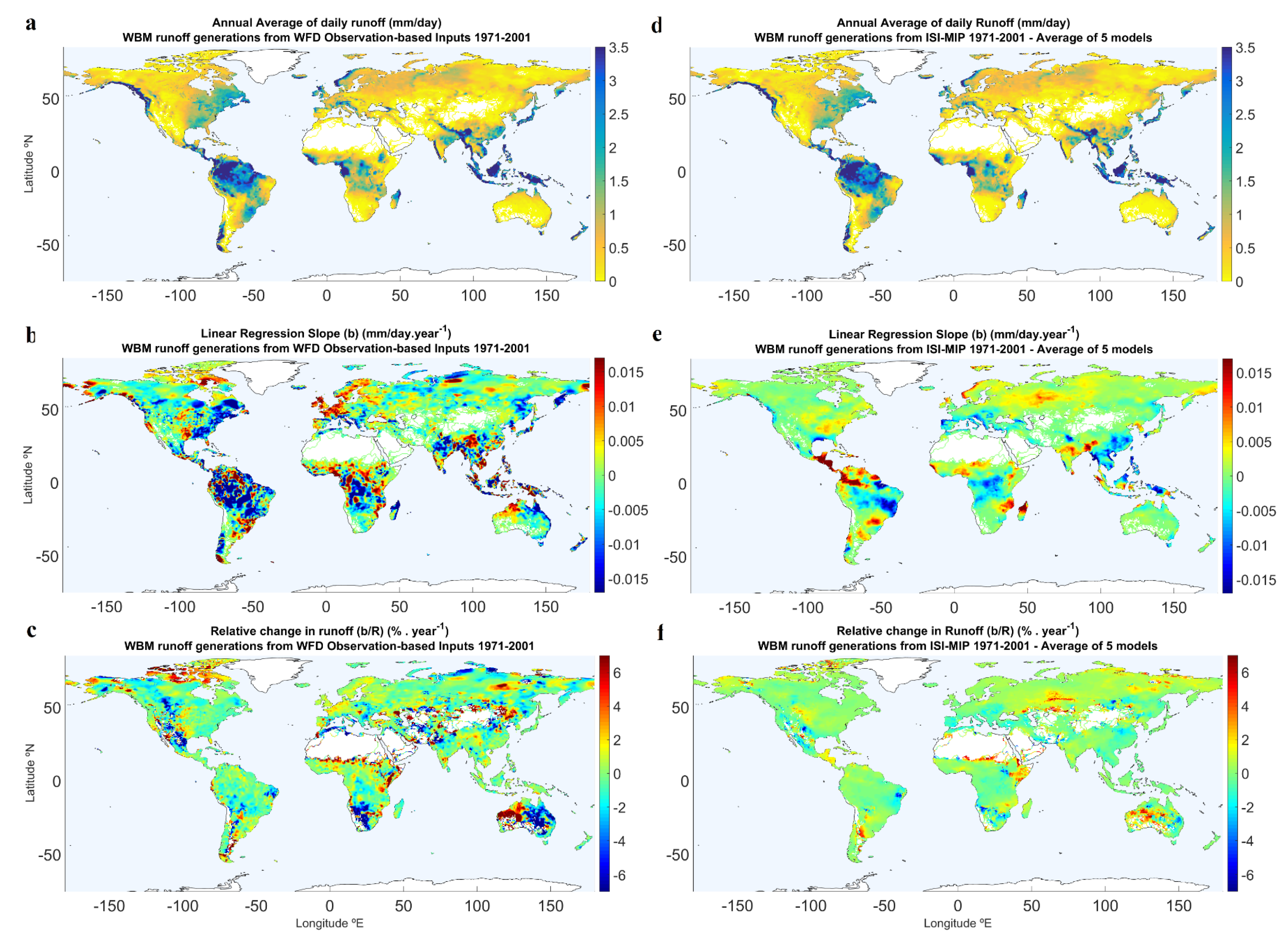
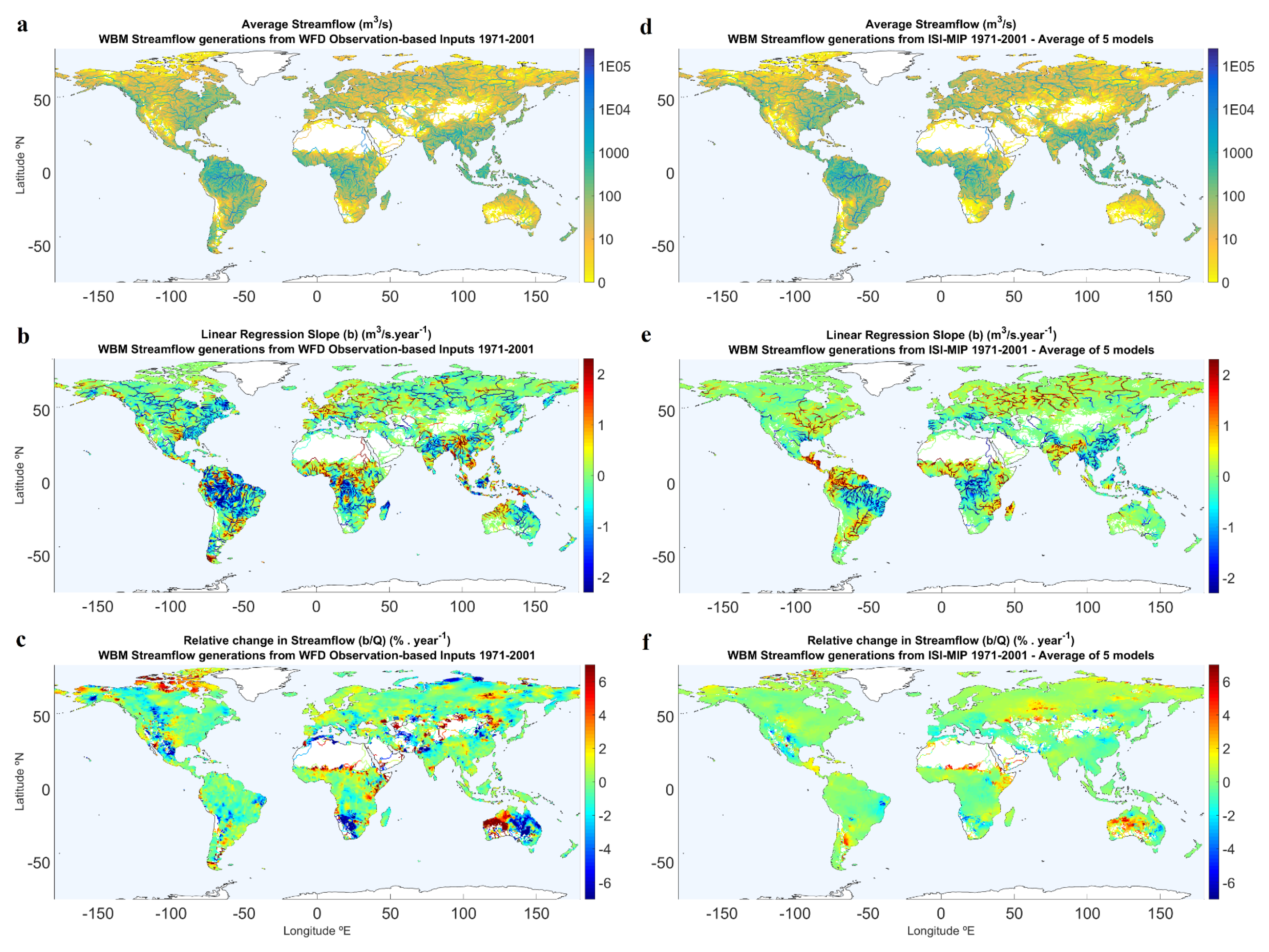
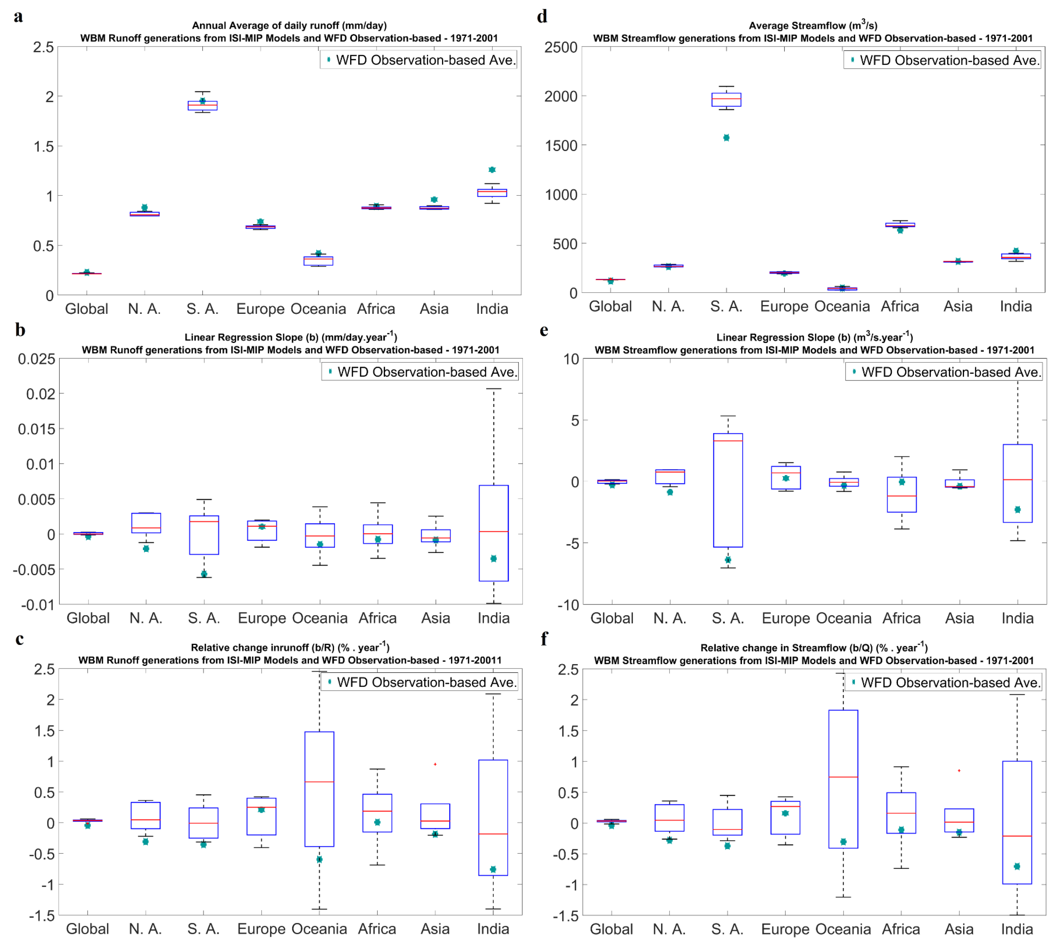
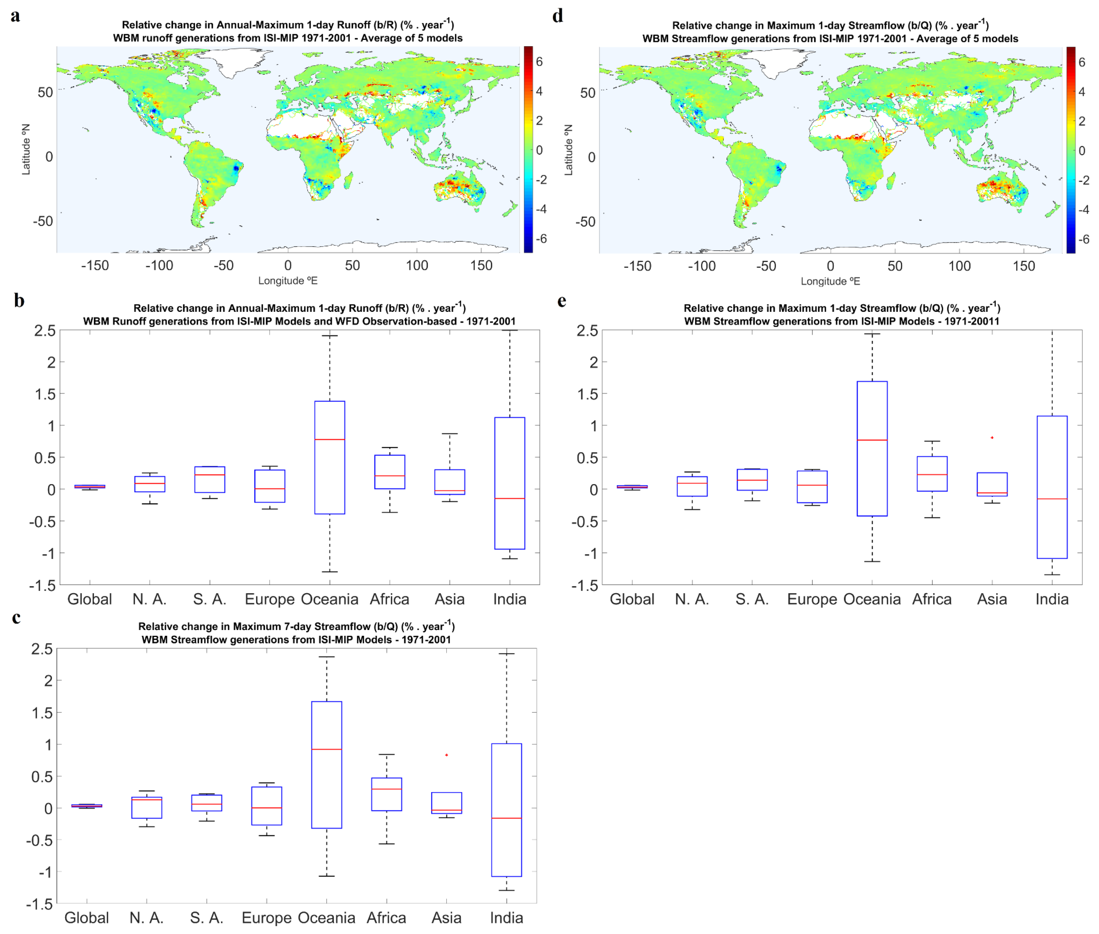
3.2. Runoff and Streamflow Trends 1971–2001 (GCMs versus Observations)

Table 2 presents the global and continental averaged trends in runoff generated by WBM, based on observation-based inputs from WFD. Results show that globally, the runoff has decreased at a rate of 0.042% per year from 1971 to 2001. Linear regression indicates that 44.8% of the grid cells show positive trend in runoff, including 5.6% that is statistically significant at 95% confidence level. The remaining 55.2% of the grid cells show negative trend, including 7.9% that is statistically significant at 95% confidence level. This implies that the trend in 86.5% of the grid cells is not significant at 95% confidence level. Table 3 presents the global average of results based on the 5 GCMs from ISI-MIP as well as observation-based simulations, for annual-mean runoff and annual-maximum daily runoff. Table 3 indicates that GCMs show good agreement with observations for the simulated average magnitude of mean runoff, which is perhaps expected given the bias-correction procedure applied to the modeled data in ISI-MIP. However, the GCM-based average shows increasing trend in mean runoff between 1971 and 2001, unlike the decreasing trend in observations. Table 3 shows that maximum runoff has also increased in GCMs, with a faster rate compared to mean runoff.
Similar to the linear regression slope (b), Qmed from Sen’s slope estimator test shows the direction and magnitude of the trend in a time series, but has the advantage of being a non-parametric method (Appendix B). The global average of Qmed is close to the average value of b obtained from the linear regression, as seen in the Table 2 and Table 3, which further supports the analysis above of the average trend magnitudes with GCMs as opposed to observation-based inputs. Values of Z-score index obtained from the Mann-Kendall method shows the non-parametric confidence level of statistical significance in the identified trends in the data. Higher values of Z correspond to higher confidence in the detected trend (Appendix A). As seen in Table 2, the global average of Z for observation-based trends is very small, further confirming the weak negative global mean trend in observation-based historical runoff, while the ISI-MIP outputs give a positive average trend (Table 3).
Figure 3a,b illustrate the global map of annual-averaged daily value of runoff from 1971 to 2001 simulated by the WBM model, based on the WFD observation-based inputs as well as from ISI-MIP models, respectively. All the maps presented for the ISI-MIP models in this study represent the average of 5 models. The two maps show signs of general agreement between the results of the GCMs (Figure 3d) and observation-based simulations (Figure 3a) in terms of the spatial distribution of annual-average runoff. Figure 3 also shows the global maps of relative change in annual-average runoff from 1971 to 2001 simulated by the WBM model based on either the inputs from the 5 ISI-MIP models (Figure 3f) or WFD observation-based data (Figure 3c).
Table 4 presents the global and continental averaged trends in observation-based streamflow (i.e., generated by WBM model, using observation-based inputs from WFD). The discharge magnitude (Q) values are per grid cell. Since both WFD and ISI-MIP dataset have the same spatial resolutions, the numbers are comparable between those two. Results show that global mean streamflow has decreased at a rate of 0.041% per year from 1971 to 2001, which is very similar to the runoff trend. Similar to those obtained from runoff data analysis, linear regression indicates that 43.4% of the grid cells show positive trend in streamflow, including 5.3% that are statistically significant at 95% confidence level. The remaining 56.6% of the grid cells show negative trend, including 8.3% that are statistically significant at 95% confidence level. This implies that trend in 86.4% of the grid cells is not significant at 95% confidence level. According to Table 4, Europe has had average streamflow increase by 4.9% over 31 years. South America, Oceania, North America, Asia and Africa have experienced decreasing trends of 11.5%, 9.4%, 8.7%, 4.7% and 3.5%, respectively.
Table 5 presents the global average of results with the 5 GCMs from ISI-MIP, as well as the global average of observation-based simulations, for annual-mean streamflow and annual-maximum 1-day streamflow. Table 5 shows that GCMs show fair agreement with observations for the simulated average magnitude of mean streamflow, as seen for average magnitude of mean runoff. However, GCMs show an average increasing trend of 0.028% per year for mean discharge, despite the decreasing trend seen for the observation-based simulations. Table 5 shows that based on the ISI-MIP output, maximum daily discharge has also increased, at a faster rate of 0.032% per year. GCMs on average show increasing trend in mean streamflow for 62.4% of the grid cells and decreasing trend for the other 37.6%. Similar to mean streamflow, extreme (annual maximum 1-day) streamflow shows increasing trend for 64.8% and decreasing trend for 35.2% of the grid cells. An assessment of the trend in annual-maximum 7-day streamflow also resulted in similar numbers (63.2% increase and 36.8% decrease). This finding is in line with the earlier study that shows increases in the 30-y return level of 5-d average peak flows (Q30) over approximately two-thirds of the global land area, in data provided by ISI-MIP from 1971 to 2000 [6].
Figure 4a,d show maps of average streamflow from 1971 to 2001 for average of the 5 GCMs from ISI-MIP and observation-based WFD data, respectively. Comparing the two maps reveals general agreement between the results of the GCM and observation-based simulations in terms of average streamflow magnitude. Figure 4 also shows global maps of relative change in streamflow from 1971 to 2001 for average of the 5 ISI-MIP models (Figure 4f), as well as observation-based WFD data (Figure 4c).
Figure 5 shows the boxplots of the results presented in Table 3 and Table 5, for mean runoff and mean streamflow. The ISI-MIP models show the opposite direction of the global average trend in runoff and streamflow, compared to observation-based simulations, as stated before. However, the disagreement is largest for the continents of North America, South America and Asia, while the observation-based average trend in Europe is closes to the median of the models (Figure 5c,f).
Comparing Table 3 and Table 5 reveals that value of relative change in streamflow for GCMs and observation-based simulations are very similar to those of runoff, which means that globally, changes in runoff are well translated to corresponding changes in streamflow. Comparing Figure 5c,f also shows such agreement in continental scale as well.
Table 4 shows an average 0.30% per year decrease in observation-based streamflow simulations in Oceania. Figure 4c shows that Australia has very mixed trends in streamflow though, as western Australia shows a significant increase in discharge while the eastern part shows significant decrease. By contrast, GCM inputs yield increase in discharge throughout Australia (Figure 4f), although uncertainty of the models in trend direction is very high for Oceania compared to the other continents (Figure 5f). As seen in Figure 4a,d, those regions have very low flow rate and hence are very sensitive, as small absolute changes in streamflow may result in high relative changes.
GCMs perform poorly in capturing the trends in regions with mixed changes in runoff and streamflow (and often low absolute runoff rates), for instance northern Africa and Australia (compare Figure 4c,f). Additionally, GCMs show higher rates of disagreement among each other in such regions, as illustrated by the wider range in the boxplots, compared to other continents (Figure 5c,f).
Figure 6 shows the maps and boxplots for extreme runoff and streamflow. Changes in extreme runoff and streamflow are very similar to those of mean runoff and streamflow, in terms of global and continental averages, although the maximum parameters show relatively faster rate of change compared to mean parameters (Table 3 and Table 5). This is similar to what is seen for precipitation in many studies, where extreme (e.g., 1-day maximum) precipitation is increasing faster than mean precipitation. Figure 6c shows relative change in annual-maximum 7-day streamflow for the ISI-MIP models, which is very similar to those in maximum 1-day streamflow (extreme streamflow) and mean streamflow.

4. Conclusions

Runoff and streamflow simulated by the WBM hydrological model based on either observation-based meteorological inputs from WATCH Forcing Data (WFD) or the bias-corrected outputs of GCMs, provided by the ISI-MIP, have been statistically analyzed. Initial comparison of the WBM streamflow with station observation streamflow data over the coterminous US shows that WBM can predict relative change in streamflow with suitable accuracy.
On global average, the mean runoff simulated based on meteorological observation-based data has decreased from 1971 to 2001. GCMs show very good agreement with observation-based estimates in case of average magnitude of mean runoff, which is expected given the bias correction procedure applied on the GCM outputs. The GCMs on average show increasing trend in mean runoff between 1971 and 2001, with an inter-model global average of 1% over that 31-year period, despite the 1.3% decrease seen in observation-based simulations. The observation-based mean streamflow has decreased by an average of 1.3% from 1971 to 2001. The GCM average shows a global averaged increase of 0.9%. In fact, each of the 5 GCMs considered yields larger global average trend for mean runoff and streamflow, compared to observation-based estimates. Results show that values of relative change in mean streamflow for GCMs are very similar to those of runoff, on global and continental scale, which means that changes in runoff have been well translated to corresponding changes in streamflow.
Relative changes in extreme runoff (and streamflow) are very similar to those of mean runoff (and streamflow), in terms of global and continental averages. However, extreme runoff (and streamflow) show relatively faster rate of change compared to mean runoff (and streamflow). Relative change in annual-maximum 7-day streamflow for the GCMs is also very similar to those of annual-maximum 1-day streamflow (extreme streamflow) and of mean streamflow.
Observation-based estimates show increasing trend in mean runoff and streamflow for about one-half of the land areas and decreasing trend for the other half (Only a minority of these gridcell-level trends are statistically significant at 95% confidence level). However, on average, mean and extreme runoff and streamflow based on GCMs show increasing trend for approximately two-thirds of the global land area and decreasing trend for the other one-third.
Results show that despite the bias-correction procedure applied on the GCM outputs in ISI-MIP, streamflow simulated based on corrected GCM outputs shows different trends compared to observation-based simulations. These differences in streamflow trends simulated over recent decades, depending on whether observation-based or bias-corrected GCM-based climate forcing is used to drive a hydrological model, deserve further investigation to understand the main contributing factors and to refine predictions for changes in water resource availability and flood hazards over the coming decades.

Acknowledgments

The authors gratefully acknowledge support from NOAA under grants NA11SEC4810004, NA12OAR4310084, NA15OAR4310080, and from PSC-CUNY Award # 68346-00 46. All statements made are the views of the authors and not the opinions of the funding agency or the U.S. government.

Author Contributions

B.A. and N.K. conceived and designed the experiment; B.A. performed the experiment and wrote the initial manuscript; B.F. developed the WBM model and provided the model runs; B.A., N.K. and B.F. analyzed the results; B.A. and N.K. wrote the paper and made the conclusions.

Conflicts of Interest

The authors declare no conflict of interest.

Appendix A. Mann-Kendall Trend Test

The MK test is a non-parametric rank based test [54,55]. The Mann-Kendall test statistic S is calculated as:
S = i = 1 n 1 j = i + 1 n s g n ( x j x i )
where n is the number of data points, xi and xj are the data values in time series i and j (j > i), respectively, and sgn(xjxi) is the sign function:
s g n ( x j     x i ) = { + 1 ,     i f    x j     x i > 0   0 ,       i f    x j     x i = 0 1 ,     i f    x j     x i < 0
The variance is computed using the equation:
V a r ( S ) = n ( n 1 ) ( 2 n + 5 ) i = 1 m t i ( t i 1 ) ( 2 t i + 5 ) 18
where n is the number of data points, m is the number of tied groups and ti is the number of ties of extent i. A tied group is a set of sample data having the same value. In cases where the sample size n > 10, the standard normal test statistic ZS is computed as:
Z S = { S 1 V a r ( S ) ,     i f    S > 0   0 ,       i f    S   =   0 S + 1 V a r ( S ) ,     i f   S <  0
The sign of ZS indicates the trend in the data series, where positive values of ZS means increasing trend, while negative ZS values show decreasing trends. For the tests at a specific α significance level, if | Z S | > Z 1 α / 2 , the null hypothesis is rejected and the time series has a statistically significant trend. Z 1 α / 2 is obtained from the standard normal distribution table, where at the 5% significance level (α = 0.05), trend is statistically significant if | Z S | > 1.96 and at the 1% significance level (α = 0.01), trend is statistically significant if | Z S | > 2.576 .

Appendix B. Sen’s Slope Estimator

The non-parametric procedure for estimating the slope of trend in the sample of N pairs of data is developed by [56] as:
Q i = x j x k j k     f o r    i = 1 , , N
where xj and xk are the data values at times j and k (j > k), respectively. N is defined as n ( n 1 ) 2 , where n is the number of time periods.
If the N values of Qi are ranked from smallest to largest, the parameter Qmed is computed as the median of the Qi vector. The Qmed sign reflects the direction of trend, while its value indicates the magnitude of the trend. To determine whether the median slope is statistically different than zero, the confidence interval of Qmed at a specific probability should be computed as follows [58,59]:
C α = Z 1 α / 2 V a r ( S )
where Var(S) is defined before and Z 1 α / 2 is obtained from the standard normal distribution table. Then, M 1 = N C α 2 and M 2 = N + C α 2 are computed. The lower and upper limits of the confidence interval, Qmin and Qmax, are the M1th largest and the (M2 + 1)th largest of the N ordered slope estimates [58]. The slope Qmed is significantly different than zero if the two limits Qmin and Qmax have the same sign.

References

  1. Allen, M.R.; Ingram, W.J. Constraints on future changes in climate and the hydrologic cycle. Nature 2002, 419, 224–232. [Google Scholar] [CrossRef] [PubMed]
  2. Held, I.M.; Soden, B.J. Robust responses of the hydrological cycle to global warming. J. Clim. 2006, 19, 5686–5699. [Google Scholar] [CrossRef]
  3. Wentz, F.J.; Ricciardulli, L.; Hilburn, K.; Mears, C. How much more rain will global warming bring? Science 2007, 317, 233–235. [Google Scholar] [CrossRef] [PubMed]
  4. Trenberth, K.E. Conceptual framework for changes of extremes of the hydrological cycle with climate change. Clim. Chang. 1999, 42, 327–339. [Google Scholar] [CrossRef]
  5. Trenberth, K.E. Changes in precipitation with climate change. Clim. Res. 2011, 47, 123–138. [Google Scholar] [CrossRef]
  6. Dankers, R.; Arnell, N.W.; Clark, D.B.; Falloon, P.D.; Fekete, B.M.; Gosling, S.N.; Heinke, J.; Kim, H.; Masaki, Y.; Satoh, Y.; et al. First look at changes in flood hazard in the Inter-Sectoral Impact Model Intercomparison Project ensemble. Proc. Natl. Acad. Sci. USA 2013, 111, 3257–3261. [Google Scholar] [CrossRef] [PubMed]
  7. Trenberth, K.E.; Dai, A.; Rasmussen, R.M.; Parsons, D.B. The changing character of precipitation. Bull. Am. Meteorol. Soc. 2003, 84, 1205–1217. [Google Scholar] [CrossRef]
  8. O’Gorman, P.A.; Schneider, T. The physical basis for increases in precipitation extremes in simulations of 21st-century climate change. Proc. Natl. Acad. Sci. USA 2009, 106, 14773–14777. [Google Scholar] [CrossRef] [PubMed]
  9. Min, S.-K.; Zhang, X.; Zwiers, F.W.; Hegerl, G.C. Human contribution to more-intense precipitation extremes. Nature 2011, 470, 378–381. [Google Scholar] [CrossRef] [PubMed]
  10. Field, C.B. Managing the Risks of Extreme Events and Disasters to Advance Climate Change Adaptation: Special Report of the Intergovernmental Panel on Climate Change; Cambridge University Press: Cambridge, UK, 2012. [Google Scholar]
  11. Solomon, S.; Qin, D.; Manning, M.; Marquis, M.; Averyt, K.; Tignor, M.M.B.; Miller, H.L.; Chen, Z. Climate Change 2007: The Physical Science Basis, Contribution of Working Group I to the Fourth Assessment Report of the Intergovernmental Panel on Climate Change; Cambridge University Press: Cambridge, UK; New York, NY, USA, 2007. [Google Scholar]
  12. Karl, T.R.; Melillo, J.M.; Peterson, T.C. Global Climate Change Impacts in the United States; Cambridge University Press: New York, NY, USA, 2009. [Google Scholar]
  13. Hansen, J.; Sato, M.; Ruedy, R.; Lo, K.; Lea, D.W.; Medina-elizade, M. Global temperature change. Proc. Natl. Acad. Sci. USA 2006, 103, 14288–14293. [Google Scholar] [CrossRef] [PubMed]
  14. Hansen, J.; Ruedy, R.; Sato, M.; Lo, K. Global surface temperature change. Rev. Geophys. 2010, 48, RG4004. [Google Scholar] [CrossRef]
  15. Stocker, T.F.; Qin, D.; Plattner, G.-K.; Tignor, M.M.B.; Allen, S.K.; Boschung, J.; Nauels, A.; Xia, Y.; Bex, V. Climate Change 2013: The Physical Science Basis. Working Group I Contribution to the Fifth Assessment Report of the Intergovernmental Panel on Climate Change-Abstract for Decision-Makers; C/O World Meteorological Organization: Geneva, Switzerland, 2013. [Google Scholar]
  16. Trenberth, K.E.; Fasullo, J.; Smith, L. Trends and variability in column-integrated atmospheric water vapor. Clim. Dyn. 2005, 24, 741–758. [Google Scholar] [CrossRef]
  17. Pall, P.; Allen, M.R.; Stone, D.A. Testing the Clausius–Clapeyron constraint on changes in extreme precipitation under CO2 warming. Clim. Dyn. 2006, 28, 351–363. [Google Scholar] [CrossRef]
  18. Allan, R.P.; Soden, B.J. Atmospheric warming and the amplification of precipitation extremes. Science 2008, 321, 1481–1484. [Google Scholar] [CrossRef] [PubMed]
  19. Lambert, F.H.; Stine, A.R.; Krakauer, N.Y.; Chiang, J.C.H. How much will precipitation increase with global warming? Eos 2008, 89, 193–200. [Google Scholar] [CrossRef]
  20. Alexander, L.V.; Zhang, X.; Peterson, T.C.; Caesar, J.; Gleason, B.; Klein Tank, A.M.G.; Haylock, M.; Collins, D.; Trewin, B.; Rahimzadeh, F.; et al. Global observed changes in daily climate extremes of temperature and precipitation. J. Geophys. Res. 2006, 111, D05109. [Google Scholar] [CrossRef]
  21. Westra, S.; Alexander, L.V.; Zwiers, F.W. Global increasing trends in annual maximum daily precipitation. J. Clim. 2013, 26, 3904–3918. [Google Scholar] [CrossRef]
  22. Asadieh, B.; Krakauer, N.Y. Global trends in extreme precipitation: Climate models versus observations. Hydrol. Earth Syst. Sci. 2015, 19, 877–891. [Google Scholar] [CrossRef]
  23. Lehmann, J.; Coumou, D.; Frieler, K. Increased record-breaking precipitation events under global warming. Clim. Chang. 2015, 132, 501–515. [Google Scholar] [CrossRef]
  24. Kharin, V.V.; Zwiers, F.W.; Zhang, X.; Wehner, M. Changes in temperature and precipitation extremes in the CMIP5 ensemble. Clim. Chang. 2013, 119, 345–357. [Google Scholar] [CrossRef]
  25. Toreti, A.; Naveau, P.; Zampieri, M.; Schindler, A.; Scoccimarro, E.; Xoplaki, E.; Dijkstra, H.A.; Gualdi, S.; Luterbacher, J. Projections of global changes in precipitation extremes from Coupled Model Intercomparison Project Phase 5 models. Geophys. Res. Lett. 2013, 40, 4887–4892. [Google Scholar] [CrossRef] [Green Version]
  26. Scoccimarro, E.; Gualdi, S.; Bellucci, A.; Zampieri, M.; Navarra, A. Heavy precipitation events in a warmer climate: Results from CMIP5 models. J. Clim. 2013, 26, 7902–7911. [Google Scholar] [CrossRef]
  27. Kharin, V.V.; Zwiers, F.W.; Zhang, X.; Hegerl, G.C. Changes in temperature and precipitation extremes in the IPCC ensemble of global coupled model simulations. J. Clim. 2007, 20, 1419–1444. [Google Scholar] [CrossRef]
  28. Zhang, X.; Zwiers, F.W.; Hegerl, G.C.; Lambert, F.H.; Gillett, N.P.; Solomon, S.; Stott, P.A.; Nozawa, T. Detection of human influence on twentieth-century precipitation trends. Nature 2007, 448, 461–465. [Google Scholar] [CrossRef] [PubMed]
  29. Chou, C.; Neelin, J. Mechanisms of global warming impacts on regional tropical precipitation. J. Clim. 2004, 17, 2688–2701. [Google Scholar] [CrossRef]
  30. Greve, P.; Orlowsky, B.; Mueller, B.; Sheffield, J.; Reichstein, M.; Seneviratne, S.I. Global assessment of trends in wetting and drying over land. Nat. Geosci. 2014, 7, 716–721. [Google Scholar] [CrossRef]
  31. Hirabayashi, Y.; Kanae, S.; Emori, S.; Oki, T.; Kimoto, M. Global projections of changing risks of floods and droughts in a changing climate. Hydrol. Sci. J. 2008, 53, 754–772. [Google Scholar] [CrossRef]
  32. Dankers, R.; Feyen, L. Climate change impact on flood hazard in Europe: An assessment based on high-resolution climate simulations. J. Geophys. Res. 2008, 113, D19105. [Google Scholar] [CrossRef]
  33. Dankers, R.; Feyen, L. Flood hazard in Europe in an ensemble of regional climate scenarios. J. Geophys. Res. 2009, 114, D16108. [Google Scholar] [CrossRef]
  34. Okazaki, A.; Yeh, P.J.-F.; Yoshimura, K.; Watanabe, M.; Kimoto, M.; Oki, T. Changes in flood risk under global warming estimated using MIROC5 and the discharge probability index. J. Meteorol. Soc. Jpn. Ser. II 2012, 90, 509–524. [Google Scholar] [CrossRef]
  35. Te Linde, A.H.; Aerts, J.C.J.H.; Bakker, A.M.R.; Kwadijk, J.C.J. Simulating low probability peak discharges for the Rhine basin using resampled climate modeling data. Water Resour. Res. 2010, 46. [Google Scholar] [CrossRef]
  36. Veijalainen, N.; Lotsari, E.; Alho, P.; Vehviläinen, B.; Käyhkö, J. National scale assessment of climate change impacts on flooding in Finland. J. Hydrol. 2010, 391, 333–350. [Google Scholar] [CrossRef]
  37. Kay, A.L.; Jones, D.A. Transient changes in flood frequency and timing in Britain under potential projections of climate change. Int. J. Climatol. 2012, 32, 489–502. [Google Scholar] [CrossRef] [Green Version]
  38. Huang, S.; Hattermann, F.F.; Krysanova, V.; Bronstert, A. Projections of climate change impacts on river flood conditions in Germany by combining three different RCMs with a regional eco-hydrological model. Clim. Chang. 2012, 116, 631–663. [Google Scholar] [CrossRef]
  39. Hagemann, S.; Chen, C.; Clark, D.B.; Folwell, S.; Gosling, S.N.; Haddeland, I.; Hanasaki, N.; Heinke, J.; Ludwig, F.; Voss, F.; et al. Climate change impact on available water resources obtained using multiple global climate and hydrology models. Earth Syst. Dyn. 2013, 4, 129–144. [Google Scholar] [CrossRef]
  40. Tang, Q.; Lettenmaier, D.P. 21st century runoff sensitivities of major global river basins. Geophys. Res. Lett. 2012, 39. [Google Scholar] [CrossRef]
  41. Hempel, S.; Frieler, K.; Warszawski, L.; Schewe, J.; Piontek, F. A trend-preserving bias correction—The ISI-MIP approach. Earth Syst. Dyn. 2013, 4, 219–236. [Google Scholar] [CrossRef]
  42. Krakauer, N.Y.; Fekete, B.M. Are climate model simulations useful for forecasting precipitation trends? Hindcast and synthetic-data experiments. Environ. Res. Lett. 2014, 9, 024009. [Google Scholar] [CrossRef]
  43. Ehret, U.; Zehe, E.; Wulfmeyer, V.; Warrach-Sagi, K.; Liebert, J. HESS Opinions “should we apply bias correction to global and regional climate model data?”. Hydrol. Earth Syst. Sci. 2012, 16, 3391–3404. [Google Scholar] [CrossRef]
  44. Hagemann, S.; Chen, C.; Haerter, J.O.; Heinke, J.; Gerten, D.; Piani, C. Impact of a statistical bias correction on the projected hydrological changes obtained from three GCMs and two hydrology models. J. Hydrometeorol. 2011, 12, 556–578. [Google Scholar] [CrossRef]
  45. Warszawski, L.; Frieler, K.; Huber, V.; Piontek, F.; Serdeczny, O.; Schewe, J. The Inter-Sectoral Impact Model Intercomparison Project (ISI-MIP): Project framework. Proc. Natl. Acad. Sci. USA 2013, 111, 1–5. [Google Scholar] [CrossRef] [PubMed]
  46. Schewe, J.; Heinke, J.; Gerten, D.; Haddeland, I.; Arnell, N.W.; Clark, D.B.; Dankers, R.; Eisner, S.; Fekete, B.M.; Colón-González, F.J.; et al. Multimodel assessment of water scarcity under climate change. Proc. Natl. Acad. Sci. USA 2014, 111, 3245–3250. [Google Scholar] [CrossRef] [PubMed] [Green Version]
  47. Vörösmarty, C.J.; Green, P.; Salisbury, J.; Lammers, R.B. Global water resources: Vulnerability from climate change and population growth. Science 2000, 289, 284–288. [Google Scholar] [CrossRef] [PubMed]
  48. Brekke, L.D.; Maurer, E.P.; Anderson, J.D.; Dettinger, M.D.; Townsley, E.S.; Harrison, A.; Pruitt, T. Assessing reservoir operations risk under climate change. Water Resour. Res. 2009, 45, 1–16. [Google Scholar] [CrossRef]
  49. Arnell, N.W. Climate change and global water resources: SRES emissions and socio-economic scenarios. Glob. Environ. Chang. 2004, 14, 31–52. [Google Scholar] [CrossRef]
  50. Oki, T.; Kanae, S. Global hydrological cycles and world water resources. Science 2006, 313, 1068–1072. [Google Scholar] [CrossRef] [PubMed]
  51. Gudmundsson, L.; Seneviratne, S.I. Towards observation-based gridded runoff estimates for Europe. Hydrol. Earth Syst. Sci. 2015, 19, 2859–2879. [Google Scholar] [CrossRef]
  52. Wisser, D.; Fekete, B.; Vorosmarty, C.J.; Schumann, A.H. Reconstructing 20th century global hydrography: A contribution to the Global Terrestrial Network-Hydrology (GTN-H). Hydrol. Earth Syst. Sci. 2010, 14, 1–24. [Google Scholar] [CrossRef]
  53. Weedon, G.P.; Gomes, S.; Viterbo, P.; Shuttleworth, W.J.; Blyth, E.; Österle, H.; Adam, J.C.; Bellouin, N.; Boucher, O.; Best, M. Creation of the WATCH Forcing Data and its use to assess global and regional reference crop evaporation over land during the twentieth century. J. Hydrometeorol. 2011, 12, 823–848. [Google Scholar] [CrossRef]
  54. Mann, H.B. Nonparametric tests against trend. Econometrica 1945, 13, 245–259. [Google Scholar] [CrossRef]
  55. Kendall, M.G. Rank Correlation Methods; Charless Griffin: London, UK, 1975. [Google Scholar]
  56. Sen, P.K. Estimates of the regression coefficient based on Kendall’s tau. J. Am. Stat. Assoc. 1968, 63, 1379–1389. [Google Scholar] [CrossRef]
  57. Hirabayashi, Y.; Mahendran, R.; Koirala, S.; Konoshima, L.; Yamazaki, D.; Watanabe, S.; Kim, H.; Kanae, S. Global flood risk under climate change. Nat. Clim. Chang. 2013, 3, 816–821. [Google Scholar] [CrossRef]
  58. Gilbert, R.O. Statistical Methods for Environmental Pollution Monitoring; John Wiley & Sons: New York, NY, USA, 1987. [Google Scholar]
  59. Hollander, M.; Wolfe, D.A. Nonparametric Statistical Methods; John Wiley & Sons: New York, NY, USA, 1973. [Google Scholar]
Figure 1. WBM model versus observations streamflow data 1971–2001 maps for Coterminous US—Log of annual-averaged daily streamflow map for observations (a) and WBM model (d), Slope of change in streamflow map for observations (b) and WBM model (e) and relative change in annual-averaged daily streamflow map for observations (c) and WBM model (f). Lower axis of the maps represents the latitude and left side axis represents the longitude of the girds.
Water 08 00189 g001
Figure 2. WBM model versus observations streamflow data 1971–2001 boxplots for Coterminous US—Log of annual-averaged daily streamflow map for observations (a), Slope of change in streamflow map for observations (b) and relative change in annual-averaged daily streamflow map for observations (c). Values larger than 99th and smaller than 1st percentile of the data (considered as the outliers) have been excluded from the plots. The boxplots show good agreement between the observations and WBM model outputs for the relative change in streamflow.
Water 08 00189 g002
Figure 3. Global maps of runoff simulations of WBM model from WFD observation-based input versus ISI-MIP model simulations input, 1971–2001—Mean runoff map for WFD (a) and ISI-MIP (d), Slope of change in mean runoff map for WFD (b) and ISI-MIP (e), and relative change in mean runoff map for WFD (c) and ISI-MIP (f). Lower side axes of the maps represent the latitudeand left side axes represent the longitude of the girds.
Water 08 00189 g003
Figure 4. Global maps of WBM streamflow generated from WFD observation-based input versus ISI-MIP inputs (average of the 5 GCMs), 1971–2001—mean streamflow map for WFD (a) and ISI-MIP (d), Slope of change in mean streamflow map for WFD (b) and ISI-MIP (e), and relative change in mean streamflow map for WFD (c) and ISI-MIP (f). The values are per grid cell.
Water 08 00189 g004
Figure 5. Boxplots of runoff and streamflow trends simulated under climate forcings from either ISI-MIP models (minimum, 25th percentile, median, 75th percentile and maximum of the 5 model runs) or WFD observation-based data (shown as blue circles) for 1971–2001 on global and continental scale—(a) annual average of runoff (mm·day−1), (b) linear regression slope of change in annual-averaged runoff (mm·day−1·year−1), (c) relative change in annual-averaged runoff (%·year−1), (d) average of discharge (m3·s−1), (e) linear regression slope of change in discharge (m3·s−1·year−1), (f) relative change in discharge (%·year−1).
Water 08 00189 g005
Figure 6. ISI-MIP global map of relative change in extreme runoff (a) and extreme streamflow (d). Boxplots of trends simulated under climate forcing from ISI-MIP models (minimum, 25th percentile, median, 75th percentile and maximum of the 5 model runs) for relative change in annual-maximum 1-day runoff (%·year−1) (b), annual-maximum 1-day streamflow (%·year−1) (e) and annual-maximum 7-day streamflow (%·year−1) (c).
Water 08 00189 g006
Table 1. Statistics of variation of streamflow trend results for observations, as well as WBM simulations in the Coterminous United States from 1971 to 2001. The observational discharge is station measurements; whereas the WBM simulated discharge average is per grid cell. WBM results are for all grid cells of the Coterminous US, as shown in Figure 1d. Ave. = Average, Min. = Minimum, Max. = Maximum, Med. = Median, St. Dev. = Standard Deviation.
Discharge Ave (Q) (m3·s−1)Slope of Change (b) (m3·s−1·year−1)Relative Change (b/Q) (%·year−1)
Obs.WBMObs.WBMObs.WBM
Grids Ave.106.4217.7−0.16−0.64−0.01−0.35
Grids Min.0.00.0−7.81−26.19−6.48−12.01
Grids Max.1776.211332.97.6623.746.8711.81
Grids Med.42.635.1−0.04−0.07−0.28−0.33
Grids St. Dev.199.5810.31.403.131.692.40
Table 2. Global and continental-averaged trend results of the WBM runoff simulations based on the WFD observation-based inputs, from 1971 to 2001. The Qmed and Z-score indices are obtained from the Sen’s slope estimator and Mann-Kendall methods, respectively, for the runoff.
Runoff Ave (R) (mm·day−1)Slope of Change (b) (mm·day−1·year−1)Relative Change (b/R) (%·year−1)Qmed (mm·day−1·year−1)Z Score (-)
Global0.23−0.00038−0.042−0.00035−0.05
North America0.88−0.00211−0.307−0.00216−0.37
South America1.95−0.00572−0.355−0.00560−0.42
Europe0.740.001040.2110.001250.23
Oceania0.42−0.00150−0.597−0.00071−0.27
Africa0.89−0.000770.009−0.00069−0.11
Asia0.96−0.00086−0.186−0.00085−0.25
India1.26−0.00351−0.758−0.00290−0.31
Table 3. Global-averaged results of mean and annual-maximum 1-day runoff trend analysis—WBM runoff simulations based on the WFD observation-based inputs as well as from the ISI-MIP (WBM model driven by GCM climate forcing), for 1971–2001. The 5 ISI-MIP models give 5 global averages, of which the minimum, maximum, median, mean, and standard deviation are presented. Ave. = Average, Min. = Minimum, Max. = Maximum, Med. = Median, St. Dev. = Standard Deviation.
Runoff Ave (R) (mm·day−1)Slope of Change (b) (mm·day−1·year−1)Relative Change (b/R) (%·year−1)Qmed (mm·day−1·year−1)Z Score (-)
Mean RunoffMax. 1d RunoffMean RunoffMax. 1d RunoffMean RunoffMax. 1d RunoffMean RunoffMax. 1d RunoffMean RunoffMax. 1d Runoff
WFD0.23-−0.00038-−0.042-−0.00035-−0.05-
ISI-MIP Ave.0.222.950.000050.003990.0310.0350.000000.002110.0110.019
ISI-MIP Min.0.212.69−0.000130.00006−0.012−0.010−0.00019−0.00070−0.0070.003
ISI-MIP Max.0.223.240.000250.007270.0610.0620.000150.004190.0380.039
ISI-MIP Med.0.212.95−0.000010.004650.0360.036−0.000050.002050.0040.015
ISI-MIP St. Dev.0.000.210.000160.002830.0260.0290.000150.001810.0190.016
Table 4. Global and continental-averaged trend results of the WBM streamflow simulations based on the WFD observation-based inputs, from 1971 to 2001. The average discharge magnitude (Q) values are per grid cell. The Qmed and Z-score indices are obtained from the Sen’s slope estimator and Mann-Kendall methods, respectively, for the streamflow.
Discharge Ave (Q) (m3·s−1)Slope of Change (b) (m3.s−1·year−1)Relative Change (b/Q) (%·year−1)Qmed (m3·s−1·year−1)Z Score (-)
Global116.50−0.28−0.041−0.29−0.06
North America262.53−0.86−0.281−0.89−0.41
South America1574.78−6.38−0.371−6.65−0.51
Europe194.210.250.1590.280.21
Oceania44.29−0.33−0.304−0.07−0.27
Africa633.57−0.04−0.112−0.13−0.11
Asia316.13−0.40−0.151−0.36−0.25
India420.07−2.30−0.704−2.40−0.46
Table 5. Global-averaged results of annual-mean and annual-maximum 1-day streamflow trend analysis—WBM streamflow simulations based on the WFD observation-based inputs as well as from the ISI-MIP (WBM model driven by GCM climate forcing), for 1971–2001. The 5 ISI-MIP models give 5 global averages, of which the minimum, maximum, median, mean, and standard deviation are presented. The average discharge magnitude (Q) values are per grid cell. Ave. = Average, Min. = Minimum, Max. = Maximum, Med. = Median, St. Dev. = Standard Deviation.
Discharge Ave (Q) (m3·s−1)Slope of Change (b) (m3·s−1·year−1)Relative Change (b/Q) (%·year−1)Qmed (m3·s−1·year−1)Z Score (-)
Mean Disch.Max. 1d Disch.Mean Disch.Max. 1d Disch.Mean Disch.Max. 1d Disch.Mean Disch.Max. 1d Disch.Mean Disch.Max. 1d Disch.
WFD116.50-−0.28-−0.041-−0.29-−0.06-
ISI-MIP Ave.132.0570.3−0.020.410.0280.032−0.040.190.010.02
ISI-MIP Min128.3531.6−0.21−0.46−0.015−0.015−0.21−0.52−0.010.00
ISI-MIP Max138.7620.90.141.130.0590.0580.150.590.030.04
ISI-MIP Med.130.6568.20.020.660.0330.031−0.020.310.000.01
ISI-MIP St. Dev.4.033.10.150.640.0270.0290.140.430.020.02

