Regional Quasi-Three-Dimensional Unsaturated-Saturated Water Flow Model Based on a Vertical-Horizontal Splitting Concept

Abstract

Due to the high nonlinearity of the three-dimensional (3-D) unsaturated-saturated water flow equation, using a fully 3-D numerical model is computationally expensive for large scale applications. A new unsaturated-saturated water flow model is developed in this paper based on the vertical/horizontal splitting (VHS) concept to split the 3-D unsaturated-saturated Richards’ equation into a two-dimensional (2-D) horizontal equation and a one-dimensional (1-D) vertical equation. The horizontal plane of average head gradient in the triangular prism element is derived to split the 3-D equation into the 2-D equation. The lateral flow in the horizontal plane of average head gradient represented by the 2-D equation is then calculated by the water balance method. The 1-D vertical equation is discretized by the finite difference method. The two equations are solved simultaneously by coupling them into a unified nonlinear system with a single matrix. Three synthetic cases are used to evaluate the developed model code by comparing the modeling results with those of Hydrus1D, SWMS2D and FEFLOW. We further apply the model to regional-scale modeling to simulate groundwater table fluctuations for assessing the model applicability in complex conditions. The proposed modeling method is found to be accurate with respect to measurements.

1. Introduction

Accurate assessment of water flow in the unsaturated-saturated porous media is critical for groundwater exploitation, groundwater resources management, crop uptake estimation, and pollution remediation [1,2,3,4]. Numerical models are effective tools to handle complicated sub-surface water flow problems of hydrologic systems, with complex and dynamic boundary conditions and heterogeneous characteristics. The complexity of subsurface systems entails not only models to reliably represent the system of interest, but also numerical solutions to efficiently solve the models for recurrent hydrological issues. A number of 3-D numerical models have been developed based on the basic idea of solving the 3-D unsaturated-saturated Richards’ equation, which is used to describe the water flow in the subsurface system. While using the 3-D model is considered to be the most rigorous approach for solving real hydrological problems [5], transient 3-D modeling is computationally expensive, especially at the regional scale, because a large amount of computational nodes and time steps are necessary to simulate the systems with sufficient accuracy [6,7]. Moreover, the numerical schemes used to solve the 3-D Richards’ equation still face a number of computational challenges, which is another hamper to the practical applications of the 3-D unsaturated-saturated model [8]. Specifically speaking, for the most popular schemes of the finite difference method (FDM) and the finite element method (FEM) adopted by MODFLOW [9] and FEFLOW [10], respectively, FDM is not flexible to handle complex domain boundaries and may yield inaccurate heads at the vicinity of the boundaries [11,12], and FEM does not maintain mass balance at the element level [13,14]. Therefore, it is necessary to simplify the 3-D models conceptually and numerically.

Considering the complexity and nonlinear intrinsic characteristics of subsurface flow systems, a variety of concepts led to the development of simplified flow models. Quasi 3-D models such as the loosely or fully coupled unsaturated-saturated models have been developed. Differing from the fully 3-D unsaturated-saturated models, which consider the water flow in three directions, the quasi-3-D models only consider the 1-D vertical infiltration in the unsaturated zone, but consider the groundwater system as 3-D flow [5,15,16]. A common feature of the quasi 3-D models is to loosely couple a 1-D vadose zone model with 3-D groundwater flow model such as the MODFLOW-type models [9]. For example, the 1-D models of SVAT, UZF1, and Hydrus1D have been integrated with MODFLOW for the unsaturated-saturated water flow modeling [7,8,17]. There are other quasi 3-D models adopting the fully coupled method to integrate the 1-D vertical unsaturated flow with 3-D water flow [3,18]. The advantages of such quasi 3-D models based on the assumption of 1-D vertical infiltration in the soil zone are that the computational cost is reduced significantly and that the convergence speed is increased, because the solution of the non-linear 3-D Richards’ equation is avoided. However, these models can only be applied to the specified conditions when the lateral transfer flow can be neglected. Otherwise, their simulations are inaccurate.

The vertical/horizontal splitting (VHS) concept is to fill the gap between computational cost and simulation accuracy. The key to the VHS concept is the decomposition of the 3-D Richards’ equation into a 1-D equation for vertical flow and a 2-D equation for depth-averaged flow. The decomposition makes it possible to obtain a faster and more flexible solution. The VHS concept was first used by Lardner and Cekirge [19] to solve a 3-D equation of tidal and storm surge. They adopted a standard 2-D algorithm for the shallow-water equations to compute the depth-averaged velocity and then to compute the vertical velocity profile. This VHS-based modeling was found to be more efficient than the 3-D modeling. Then, Tsai et al. [20] developed a layered and regional land subsidence model based on the VHS concept. Similar models have been developed to simulate the sediment transport in the coastal region by coupling a 2-D model with an additional 1-D vertical profile model [21,22,23]. Lin et al. [24] were the first to use the VHS concept to simplify the 3-D saturated water flow equation to a 2-D horizontal water flow equation and to integrate the horizontal flow with the vertical flux. However, the model was only suitable to a horizontal aquifer with small slopes and was invalid when the aquifer was inclined. Paulus et al. [25] proposed an innovative 3-D unsaturated flow model by decoupling the 3-D Richards’ equation into a 1-D vertical equation and a 2-D depth-integrated horizontal equation. The model was demonstrated to be efficient. However, this model cannot be used for heterogeneous soils and the FDM used in the model hampers its application to irregular domains. More studies are needed to make a full use of the VHS concept for its high efficiency to solve a 2-D horizontal water flow equation and a 1-D vertical water flow equation. This is the case in comparison with the fully 3-D equation, especially the solution of the complete 3-D equation on large-scale basins, which leads to the very huge non-linear systems, whose numerical solution is very costly. Another advantage of the VHS-based modeling is that, after splitting the 3-D Richards’ equation to horizontal and vertical equations, the equations can be solved by using different numerical schemes suitable to the equations.

The objective of this paper is to present a VHS-based 3-D unsaturated-saturated water flow model to split the 3-D unsaturated-saturated water flow to the 2-D horizontal flow described by a 2-D equation and the 1-D flow described by a 1-D equation. Different optional methods are used for the two equations. The 2-D horizontal equation represents the lateral flow in the horizontal plane of average head gradient, which is calculated by the water balance method. In addition, the 1-D vertical equation is discretized by the FDM to integrate the different horizontal layers. The two equations are solved simultaneously by coupling them into a unified nonlinear system with a single matrix. The efficiency and accuracy of the developed model and its computer code are evaluated by using three synthetic cases represented the 1-D infiltration flow, 2-D lateral flow, and 3-D well flow. Furthermore, the model applicability and efficiency are examined by simulating groundwater flow under complicated boundary conditions in a regional-scale case.

2. Mathematical and Numerical Method

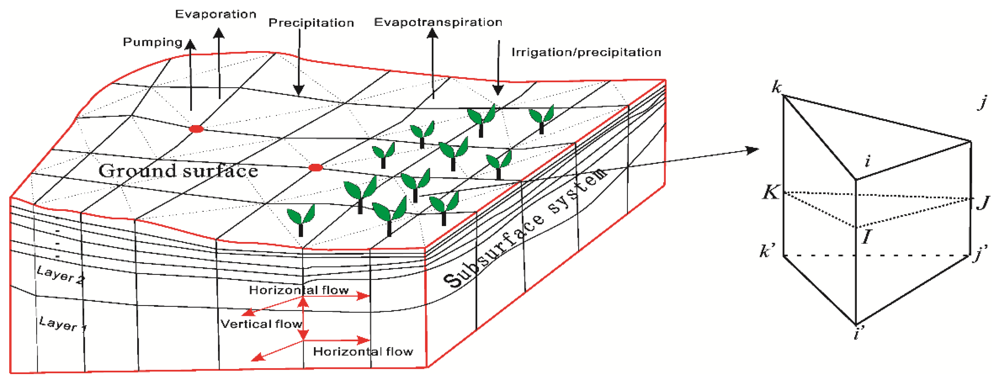
2.1. Discretization of the Aquifer

The model is established firstly by separating the 3-D aquifer into different layers. Each layer is divided into triangular prism elements. The horizontal plane of average head gradient is derived to represent the average horizontal flow in the triangular prism element. The aquifer domain, the divided triangular prism element and the horizontal plane of average head gradient are shown in Figure 1. The governing 3-D Richards’ equation is split into a 2-D horizontal water flow equation based on the horizontal plane of average head gradient in the triangular prism element and a 1-D vertical water equation. The water balance method is used to calculate the horizontal flow flux and the FDM is adopted for calculating the vertical flow flux. The horizontal flow and the 1-D vertical flow are integrated into one unified matrix and then solved simultaneously. The details are shown in the next sections.

2.2. The Governing Equations

The general 3-D unsaturated-saturated water flow is represented as follows:

$$\frac{\partial \mathsf{\theta }}{\partial t}=\frac{\partial }{\partial x_i}\left[K\frac{\partial H}{\partial x_j})\right]-S$$

(1)

where θ is the volumetric water content [–]; t is the time [T]; K is the hydraulic conductivity as a function of pressure head [L T⁻¹]; H is the hydraulic head [L]; x_i, x_j (i, j = x, y, z) are the coordinates in the x, y and z directions [L]; S is the sink or source term [T⁻¹].

Considering the first left item of Equation (1) as

$$\frac{\partial \mathsf{\theta }}{\partial t}=C(h)\frac{\partial H}{\partial t}$$

(2)

where C(h) is the soil water capacity [L⁻¹] and can be calculated as

$$C(h)=\frac{\mathsf{\theta }}{n}\mathsf{\mu }+\frac{\mathrm{d}\mathsf{\theta }}{\mathrm{d}h}$$

(3)

where µ is the elastic storage coefficient [L⁻¹]; n is the soil porosity [–]; h is the pressure head [L].

In the saturated zone, dθ/dh can be ignored, and θ/n equals 1.0. The hydraulic conductivity is the saturated hydraulic conductivity K_s. Therefore, for the saturated water flow, the water flow Equation (1) can be simplified as

$$\mathsf{\mu }\frac{\partial H}{\partial t}=\frac{\partial }{\partial x_i}\left[K_s\frac{\partial H}{\partial x_j}\right]-S$$

(4)

In the unsaturated zone, θ/n × µ can be ignored. Then, C(h) equals to dθ/dh, and the hydraulic conductivity is a function of pressure head. These two items can be calculated according to the modified van Genuchten model [26], shown as Equations (6) and (7). Then, in the unsaturated zone, the water flow Equation (1) can be rewritten as

$$C(h)\frac{\partial H}{\partial t}=\frac{\partial }{\partial x_i}\left[K(h)\frac{\partial H}{\partial x_i}\right]-S$$

(5)

Therefore, the saturated water flow Equation (4) and the unsaturated water flow Equation (5) have the same equation form but with their specified coefficients as

$$C=\{\begin{array}{ll}-mn{\mathsf{\alpha }}^n({\mathsf{\theta }}_m-{\mathsf{\theta }}_a){\left[1+{(\mathsf{\alpha }h)}^n\right]}^{-m-1}{h}^{n-1}& (\text{in the unsaturated zone})\\ \hspace{1em}\mathsf{\mu }& (\text{in the saturated zone})\end{array}$$

(6)

$$K=\{\begin{array}{ll}{K}_s{\left(\frac{\mathsf{\theta }-{\mathsf{\theta }}_r}{{\mathsf{\theta }}_s-{\mathsf{\theta }}_r}\right)}_{}^{1/2}{\left[1-{\left({\left(1-\frac{\mathsf{\theta }-{\mathsf{\theta }}_r}{{\mathsf{\theta }}_s-{\mathsf{\theta }}_r}\right)}_{}^{1/m}\right)}^m\right]}^2& (\text{in the unsaturated zone})\\ \hspace{1em}{K}_s& (\text{in the saturated zone})\end{array}$$

(7)

where θ_m is the fictitious saturated water content in the soil water retention function [–]; θ_r is the residual water content [–]; θ_a is the parameter in the soil water retention function [–]; θ_s is the saturated water content [–]; K_s is the saturated hydraulic conductivity [L T⁻¹]; α is the coefficient in the soil water retention function [L⁻¹]; m, n are the exponents in the soil water retention function [–].

2.3. Depth-Averaged Water Flow Equation

Considering one horizontal layer, the depth-average 2-D equation can be obtained by integrating the 3-D flow equation over the vertical direction, which yields

$${\int }_{z_i\left(x,y\right)}^{z_{i+1}\left(x,y\right)}C\frac{\partial H}{\partial t}\mathrm{d}z={\int }_{z_i\left(x,y\right)}^{z_{i+1}\left(x,y\right)}\left[\frac{\partial }{\partial x}\left(K\frac{\partial H}{\partial x}\right)+\frac{\partial }{\partial y}\left(K\frac{\partial H}{\partial y}\right)+\frac{\partial }{\partial z}\left(K\frac{\partial H}{\partial z}\right)\right]\mathrm{d}z-{\int }_{z_i\left(x,y\right)}^{z_{i+1}\left(x,y\right)}S\mathrm{d}z$$

(8)

where z_i(x,y) and z_i+1(x,y) are the bottom and upper boundary, respectively, of the aquifer. By assuming B = z_i+1(x,y)- z_i(x,y) and employing Leibnitz rule, we rewrite Equation (8) as

$$B\overline{C}\frac{\partial \overline{H}}{\partial t}=B\frac{\partial }{\partial x}\left(K\frac{\partial \overline{H}}{\partial x}\right)+B\frac{\partial }{\partial y}\left(K\frac{\partial \overline{H}}{\partial y}\right)+{V_z|}_{z_i}{-V_z|}_{z_{i+1}}-B\overline{S}$$

(9)

where $\overline{C}$, $\overline{H}$ and $\overline{S}$ denote the property defined in the xy-plane (herein we call this special plane the horizontal plane of average head gradient, and the derivation can be found in Section 2.4.). The ${V_z|}_{z_{i+1}}$ and ${V_z|}_{z_i}$ denote the water flux vectors at the upper and bottom aquifer, respectively.

2.4. The Horizontal Plane of Average Head Gradient in the Triangular Prism Element

The horizontal plane of average head gradient in an irregular triangular prism element means the average lateral head gradient in this irregular triangular prism element, and it is used to approximately calculate the net lateral flux. There are two assumptions made to derive the horizontal plane of average head gradient, (1) the head varies linearly between the upper and bottom nodes within the element; (2) the head in the horizontal plane is linearly interpolated by the head of three nodes I, J, K, which lead to

$$H_P={\mathsf{\beta }}_P{H}_p+(1-{\mathsf{\beta }}_P)H_{p’}$$

(10)

$$H\left(x,y,t\right)=\frac{1}{2\Delta }[\left(a_{i}x+b_{i}y+d_i\right)H_I+\left(a_{j}x+b_{j}y+d_j\right)H_J+\left(a_{k}x+b_{k}y+d_k\right)H_K]$$

(11)

where H_P (P = I, J, K) are the head of three nodes in the horizontal plane of triangular prism element IJK [L]; H_p (p = i, j, k) and H_p’ (p’ = i’, j’, k’) are the head of six nodes in the triangular prism element; Δ is the area of the triangle IJK; $a_i=y_j-y_k$; $b_i=x_k-x_j$; $d_i=x_j{y}_k-x_k{y}_j$; $a_j=y_k-y_i$; $b_j=x_i-x_k$; $d_j=x_k{y}_i-x_i{y}_k$; $a_k=y_i-y_j$; $b_k=x_j-x_i$; $d_k=x_i{y}_j-x_j{y}_i$; x_i, y_i (i = i, j, k) are the x and y coordinates of node i, j and k [L]; β_P (P=I, J, K) are calculated as

$$\begin{array}{l}{\mathsf{\beta }}_I=(\overline{z}-z_{i’})/(z_i-z_{i’})\\ {\mathsf{\beta }}_J=(\overline{z}-z_{j’})/(z_j-z_{j’})\\ {\mathsf{\beta }}_K=(\overline{z}-z_{k’})/(z_k-z_{k’})\end{array}$$

(12)

where z_i (i = i, i’, j, j’, k, k’) are the z-coordinates of six nodes in the triangular prism element [L]; and $\overline{z}$ is the z-coordinate of the horizontal plane of average head gradient [L].

Derived from Equation (11), the head gradients along the x- and y-directions can be calculated. Since they have a similar form, only the head gradient along the x-direction in the plane IJK is shown here in detail,

$$\frac{\partial H}{\partial x}=\frac{1}{2\Delta }[\left(a_i{A}_{ii’}+a_j{A}_{jj’}+a_k{A}_{kk’}\right)z+\left(a_i{H}_{ii’0}+a_j{H}_{jj’0}+a_k{H}_{kk’0}\right)]$$

(13)

where,

$$\Delta =\frac{1}{2}\left(a_j{b}_k-a_k{b}_j\right)$$

(14)

$$\begin{array}{l}{A}_{ii’}=\left(\frac{H_i-H_{i’}}{z_i-z_{i’}}\right),H_{ii’0}=H_i-\frac{H_i-H_{i’}}{z_i-z_{i’}}{z}_i{z}_i<z<z_{i^{’}}\\ A_{jj’}=\frac{H_j-H_{j’}}{z_j-z_{j’}},H_{jj’0}=H_j-\frac{H_j-H_{j’}}{z_j-z_{j’}}{z}_j{z}_j<z<z_{j^{’}}\\ A_{kk’}=\frac{H_k-H_{k’}}{z_k-z_{k’}},H_{kk’0}=H_k-\frac{H_k-H_{k’}}{z_k-z_{k’}}{z}_k{z}_k<z<z_{k^{’}}\end{array}$$

(15)

In the triangular prism element ijki’j’k’, the horizontal plane of average head gradient can be calculated as

$$\begin{array}{l}\frac{{\int }_{z_{k’}}^{z_i}\left(\frac{\partial H}{\partial x}S\right)dz}{{\displaystyle {\int }_{z_{k’}}^{z_i}S}dz}=\frac{1}{2\Delta }\left(a_i{A}_{ii’}+a_j{A}_{jj’}+a_k{A}_{kk’}\right)\times \frac{\left\{\begin{array}{l}\frac{\left(a_j{b}_k-a_k{b}_j\right)}{24}\left[\left(z_i-z_j\right)\left(z_i+3z_j\right)-\left(z_{i’}-z_{k’}\right)\left(z_{i’}+3z_{k’}\right)\right]\\ +\Delta \frac{\left(z_j-z_{i’}\right)\left(z_j+z_{i’}\right)}{2}+\Delta \frac{\left(z_{i’}-z_{k’}\right)\left(z_{i’}+z_{k’}\right)}{2}\end{array}\right\}}{\frac{\left(a_j{b}_k-a_k{b}_j\right)}{2}\frac{\left[\left(z_i-z_j\right)-\left(z_{i’}-z_{k’}\right)\right]}{3}+\Delta \left(z_j-z_{k’}\right)}\\ +\frac{1}{2\Delta }\left(a_i{H}_{ii’0}+a_j{H}_{jj’0}+a_k{H}_{kk’0}\right)\end{array}$$

(16)

By combined consideration of Equation (11) and Equation (16), the vertical coordinate of the horizontal plane of average head gradient IJK in the triangular prism element ijki’j’k’ is given as

$$\overline{z}=\frac{\left\{\frac{1}{12}\left[\left(z_i-z_j\right)\left(z_i+3z_j\right)-\left(z_{i’}-z_{k’}\right)\left(z_{i’}+3z_{k’}\right)+\frac{\left(z_j-z_{i’}\right)\left(z_j+z_{i’}\right)}{2}+\frac{\left(z_{i’}-z_{k’}\right)\left(z_{i’}+z_{k’}\right)}{2}\right]\right\}}{\left\{\frac{\left[\left(z_i-z_j\right)-\left(z_{i’}-z_{k’}\right)\right]}{3}+\left(z_j-z_{k’}\right)\right\}}$$

(17)

2.5. The Discretization of the Lateral flow Equation

As shown in Equation (9), the item $B\frac{\partial }{\partial x}\left(K\frac{\partial \overline{H}}{\partial x}\right)+B\frac{\partial }{\partial y}\left(K\frac{\partial \overline{H}}{\partial y}\right)$ means the lateral flow. Since B is the thickness of the triangular prism element and can be considered as constant, the key to calculate the lateral flow is to discretize the $\frac{\partial }{\partial x}\left(K\frac{\partial \overline{H}}{\partial x}\right)+\frac{\partial }{\partial y}\left(K\frac{\partial \overline{H}}{\partial y}\right)$ term. The water balance analysis method is adopted, and the net lateral flux from the plane IJK to node I is expressed as follows [27]:

$$Q_I=-\frac{K}{4\Delta }\left[\left(b_i{}^2+a_i{}^2\right)H_I+\left(b_j{b}_i+a_j{a}_i\right)H_J+\left(b_k{b}_i+a_k{a}_i\right)H_K\right]$$

(18)

where Δ is the area of triangle IJK; and a_p, b_p (p = i, j, k) have the same meaning as mentioned above. It should be noted that the x and y coordinates of the three nodes in the plane IJK equal those in the upper or bottom surface of the triangular prism element. In the triangular prism element ijki’j’k’, the lateral flux to node i can be calculated by the lateral flux to node I and the thickness of the control volume of node i, which is one half the average thickness of the element. Then, by comprehensive consideration with the assumption that the head varies linearly with the depth in each triangular prism element shown in Equation (10) and Equation (18), the lateral flux to node i in the element ijki’j’k’ can be expressed as

$$Q_i=-\frac{\overline{K}\times B}{8\Delta }[P_{ii}{\mathsf{\beta }}_I{H}_i+P_{ii}(1-{\mathsf{\beta }}_I)H_i+P_{ij}{\mathsf{\beta }}_J{H}_j+P_{ij}(1-{\mathsf{\beta }}_J)H_{j’}+P_{ik}{\mathsf{\beta }}_K{H}_k+P_{ik}(1-{\mathsf{\beta }}_K)H_{K’}]$$

(19)

where $\overline{K}$ is the mean hydraulic conductivity of the triangular prism element; $a_i{}^2+b_i{}^2=P_{ii}$, $a_i{a}_j+b_i{b}_j=P_{ij}$, $a_i{a}_k+b_i{b}_k=P_{ik}$.

2.6. The Discretization of the Water Mass Change Item

The first item in Equation (9) characterizes the capacity of an aquifer to release or store water in response to a unit hydraulic head change. The water flow change in the control volume of node i in the triangular prism element can be expressed as

$$Q_c=\frac{\Delta }{3}\frac{\overline{C}B}{2}\frac{\Delta H_i}{\Delta t}$$

(20)

The water mass change in the control volume of node i in the triangular prism element from the source/sink items can be calculated by

$$Q_s=\frac{B}{2}\times \frac{\Delta }{3}\times \overline{S}=\frac{1}{6}\Delta \times B\times \overline{S}$$

(21)

2.7. The Element Matrices

Equations (19), (20) and (21) provide, respectively, the lateral flow, water mass change from a unit head change and source/sink items in the control volume of node i in the element ijki’j’k’. Similarly, these items in the control volume for the other five nodes can be calculated. Then, we obtain the discretized Richards’ equation in terms of matrices in the element ijki’j’k’ as follows (excluding the vertical flux, which will be calculated in the next section),

$$\begin{array}{l}\frac{\overline{K}B}{8\Delta }\left[\begin{array}{cccccc}{P}_{ii}{\mathsf{\beta }}_I& P_{ij}{\mathsf{\beta }}_J& P_{ik}{\mathsf{\beta }}_K& P_{ii}(1-{\mathsf{\beta }}_I)& P_{ij}(1-{\mathsf{\beta }}_J)& P_{ik}(1-{\mathsf{\beta }}_K)\\ P_{ji}{\mathsf{\beta }}_I& P_{jj}{\mathsf{\beta }}_J& P_{jk}{\mathsf{\beta }}_K& P_{ji}(1-{\mathsf{\beta }}_I)& P_{jj}(1-{\mathsf{\beta }}_J)& P_{jk}(1-{\mathsf{\beta }}_K)\\ P_{ki}{\mathsf{\beta }}_I& P_{kj}{\mathsf{\beta }}_J& P_{kk}{\mathsf{\beta }}_K& P_{ki}(1-{\mathsf{\beta }}_I)& P_{kj}(1-{\mathsf{\beta }}_J)& P_{kk}(1-{\mathsf{\beta }}_K)\\ P_{ii}{\mathsf{\beta }}_I& P_{ij}{\mathsf{\beta }}_J& P_{ik}{\mathsf{\beta }}_K& P_{ii}(1-{\mathsf{\beta }}_I)& P_{ij}(1-{\mathsf{\beta }}_J)& P_{ik}(1-{\mathsf{\beta }}_K)\\ P_{ji}{\mathsf{\beta }}_I& P_{jj}{\mathsf{\beta }}_J& P_{jk}{\mathsf{\beta }}_K& P_{ji}(1-{\mathsf{\beta }}_I)& P_{jj}(1-{\mathsf{\beta }}_J)& P_{jk}(1-{\mathsf{\beta }}_K)\\ P_{ki}{\mathsf{\beta }}_I& P_{kj}{\mathsf{\beta }}_J& P_{kk}{\mathsf{\beta }}_K& P_{ki}(1-{\mathsf{\beta }}_I)& P_{kj}(1-{\mathsf{\beta }}_J)& P_{kk}(1-{\mathsf{\beta }}_K)\end{array}\right]\left[\begin{array}{c}{H}_i\\ H_j\\ H_k\\ H_{i’}\\ H_{j’}\\ H_{k’}\end{array}\right]\\ +\frac{\overline{C}\Delta B}{6}\left[\begin{array}{cccccc}1& & & & & \\ & 1& & & & \\ & & 1& & & \\ & & & 1& & \\ & & & & 1& \\ & & & & & 1\end{array}\right]\left[\begin{array}{c}\mathrm{d}{H}_i/\mathrm{d}t\\ \mathrm{d}{H}_j/\mathrm{d}t\\ \mathrm{d}{H}_k/\mathrm{d}t\\ \mathrm{d}{H}_{i’}/\mathrm{d}t\\ \mathrm{d}{H}_{j’}/\mathrm{d}t\\ \mathrm{d}{H}_{k’}/\mathrm{d}t\end{array}\right]-\frac{\Delta B\overline{S}}{6}\left[\begin{array}{c}1\\ 1\\ 1\\ 1\\ 1\\ 1\end{array}\right]=0\end{array}$$

(22)

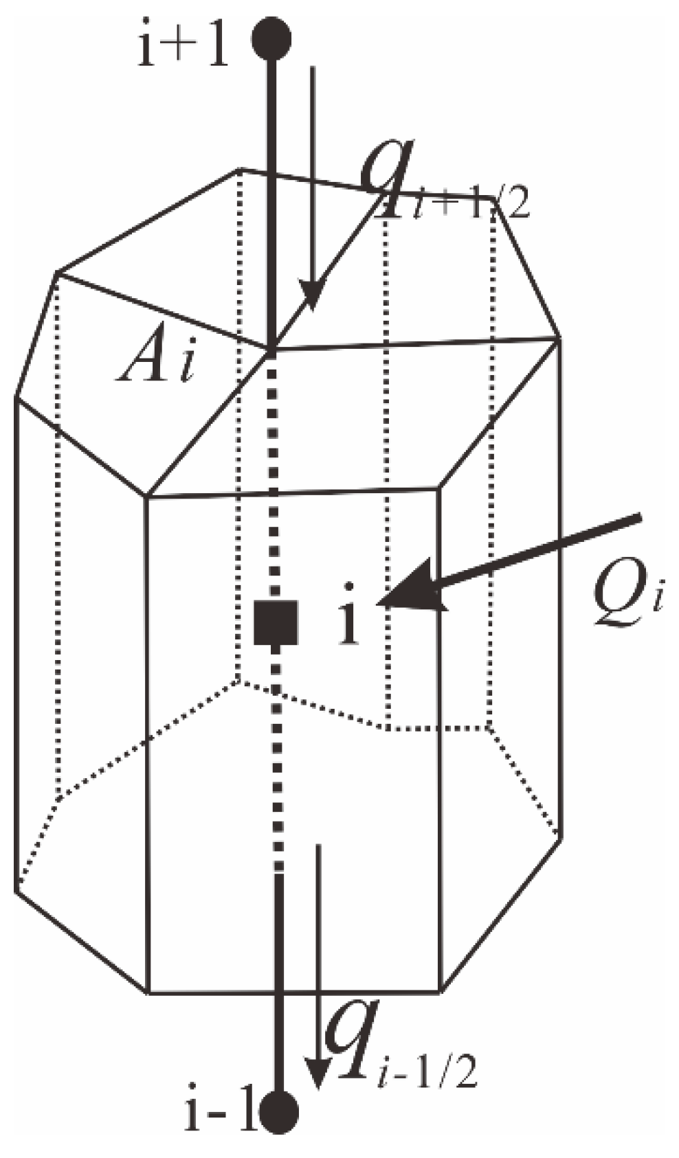
2.8. Coupling Horizontal Flow with the Vertical Fluxes

The vertical flow flux is represented by ${V_z|}_{z_i}-{V_z|}_{z_{i+1}}$ in Equation (9). As specified in the element ijki’j’k’, we calculate the net vertical flow to the control volume of node i as an example (see Figure 2), by using FDM. When the node i is located between the ground surface and the bottom of the aquifer, the vertical flux to node i can be calculated as,

$$Q_v=-A_i\left(q_{i-1/2}-q_{i+1/2}\right)=\frac{A_i\overline{K_{i,i-1}}}{B_{i,i-1}}{H}_{i-1}-\left(\frac{A_i\overline{K_{i,i+1}}}{B_{i,i+1}}+\frac{A_i\overline{K_{i,i-1}}}{B_{i,i-1}}\right)H_i+\frac{A_i\overline{K_{i,i+1}}}{B_{i,i+1}}{H}_{i+1}$$

(23)

where q_i+1/2 and q_i−1/2 are the upper and bottom fluxes, respectively; A_i is the control area of node i in the triangular prism element [L²]. Node i−1 and node i+1 are the adjacent nodes to the node i in the vertical direction; $\overline{K_{i,i-1}}$ is the geometric average hydraulic conductivities of the nodes i and i−1; and B_i,i−1 is the distance between the nodes i and i−1. $\overline{K_{i,i+1}}$ and B_i,i+1 are defined in the same way.

When the node i is located at the ground surface, q_i+1/2 becomes zero and the vertical flux can be calculated as

$$Q_{v\_upper}=-A_i\left(q_{i-1/2}\right)=\frac{A_i\overline{K_{i,i-1}}}{B_{i,i-1}}{H}_{i-1}-\frac{A_i\overline{K_{i,i-1}}}{B_{i,i-1}}{H}_i$$

(24)

When the node i is located at the bottom of the aquifer, q_i+1/2 becomes zero and then the vertical flux will be

$$Q_{v\_Bottom}=-A_i\left(-q_{i+1/2}\right)=-\frac{A_i\overline{K_{i,i+1}}}{B_{i,i+1}}{H}_i+\frac{A_i\overline{K_{i,i+1}}}{B_{i,i+1}}{H}_{i+1}$$

(25)

2.9. Illustrative Example to Elaborate the Coupling Method of Horizontal Layers

The spatial discretized Equation (22) is further discretized by the implicit method temporally to form the calculation matrix; then, the unified matrix of the unsaturated-saturated water flow is developed by assembling the vertical fluxes represented by Equations (23)–(25) between each layer. A two layer aquifer with 3n nodes is presented to show how the coupling procedure implements to form the global matrix. For this case, the global matrix is (3n) × (3n) as shown in Equation (26). The small letters $w_i^j$, b_i (i, j=1, 2, …, 3n) represent the items formed by temporally discretizing Equation (22) with the implicit method, and the capital letters $W_i^j$ (i, j = n+1, n+2, …, 2n+1) represent the modified items according to Equations (23), (24) and (25),

$$\left[\begin{array}{ccccccccc}{W}_1^1& \cdots & w_1^n& W_1^{n+1}& & & & & \\ ⋮& \ddots & ⋮& & \ddots & & & & \\ w_n^1& \dots & W_n^n& & & W_n^{2n}& & & \\ W_{n+1}^1& & & W_{n+1}^{n+1}& \cdots & w_{n+1}^{2n}& W_{n+1}^{2n+1}& & \\ & \ddots & & ⋮& \ddots & ⋮& & \ddots & \\ & & W_{2n}^n& w_{2n}^{n+1}& \cdots & W_{2n}^{2n}& & & W_{2n}^{3n}\\ & & & W_{2n+1}^{n+1}& & & W_{2n+1}^{2n+1}& \cdots & w_{2n+1}^{3n}\\ & & & & \ddots & & ⋮& \ddots & ⋮\\ & & & & & W_{3n}^{2n}& w_{3n}^{2n+1}& \dots & W_{3n}^{3n}\end{array}\right]\left[\begin{array}{c}{H}_1\\ ⋮\\ H_n\\ H_{n+1}\\ ⋮\\ H_{2n}\\ H_{2n+1}\\ ⋮\\ H_{3n}\end{array}\right]=\left[\begin{array}{c}{b}_1\\ ⋮\\ b_n\\ b_{n+1}\\ ⋮\\ b_{2n}\\ b_{2n+1}\\ ⋮\\ b_{3n}\end{array}\right]$$

(26)

According to Equation (23), $W_j^j(j=n+1,\cdots ,2n)$ items for the nodes between the ground surface and the aquifer bottom are modified by

$$W_j^j=w_j^j+\left(\frac{A_j\overline{K_{j,j+n}}}{B_{j,j+n}}+\frac{A_j\overline{K_{j,j-n}}}{B_{j,j-n}}\right)$$

(27)

$$W_j^{j-n}=w_j^{j-n}-\frac{A_j\overline{K_{j,j-n}}}{B_{j,j-n}}$$

(28)

$$W_j^{n+j}=w_j^{n+j}-\frac{A_j\overline{K_{j,j+n}}}{B_{j,j+n}}$$

(29)

According to Equation (24), $W_j^j(j=2n+1,\cdots ,3n)$ items for the ground surface nodes are modified by

$$W_j^j=w_j^j+\frac{A_j\overline{K_{j,j-n}}}{B_{j,j-n}}$$

(30)

$$W_j^{j-n}=w_j^{j-n}-\frac{A_j\overline{K_{j,j-n}}}{B_{j,j-n}}$$

(31)

According to Equation (25), $W_j^j(j=1,\cdots ,n)$ items for the bottom nodes are modified by

$$W_j^j=w_j^j+\frac{A_j\overline{K_{j,j+n}}}{B_{j,j+n}}$$

(32)

$$W_j^{n+j}=w_j^{n+j}-\frac{A_j\overline{K_{j,j+n}}}{B_{j,j+n}}$$

(33)

3. Boundary Conditions and Source/Sink Items

The model can handle various kinds of boundary conditions and source/sink items, such as the first- and second-kind boundary conditions, root uptake, pumping well, and atmosphere boundary conditions (e.g., precipitation and evaporation or evapotranspiration). The details are as follows.

(1)

First-kind boundary condition:

$$H_1(x,y,z,t)=\mathsf{\phi }(x,y,z,t)(x,y,z)\in {\Gamma }_D$$

(34)

where $\mathsf{\phi }$ is the prescribed head in the boundary [L].

(2)

Second-kind boundary condition:

$$K\frac{\partial H}{\partial n}=q(x,y,z,t)(x,y,z)\in {\Gamma }_N$$

(35)

where q is the prescribed flow flux in the boundary [L² T⁻¹].

(3)

Pumping well:

$$Q_{p,i}=\frac{L_i{K}_{ix}}{{\displaystyle \sum \left(L_i{K}_i{}_x\right)}}{Q}_w{\mathsf{\beta }}_I,Q_{p,i’}=\frac{L_i{K}_{ix}}{{\displaystyle \sum \left(L_i{K}_i{}_x\right)}}{Q}_w(1-{\mathsf{\beta }}_I)$$

(36)

where Q_p,i and Q_p,i’ are the pumping rate of the nodes i and i’, respectively [L³ T⁻¹]; L_i is the length of the pumping well filtration in the i-th layer [L]; and Q_w is the total pumping rate [L³ T⁻¹]; β_I is calculated by Equation (12). If the drawdown caused by pumping is very large to disconnect the nodes with the groundwater system, the pumping rate will be set as zero without extraction.

(4)

Root uptake

The sink term of root uptake, S, is calculated by [28] as

$$S=\mathsf{\alpha }(h)S_p$$

(37)

where α(h) is a pressure response function of root uptake [–], and S_p is the potential water uptake by plant [T⁻¹].

(5)

Atmosphere boundary conditions

The model can handle daily changing atmosphere boundary conditions such as precipitation rate and evapotranspiration rate. The precipitation rate is input according to the climate information. There are two ways to handle the evapotranspiration boundary. One is pre-processing the evapotranspiration rate as input information. The input evapotranspiration rate (ET) is calculated by multiplying the daily evaporation from water surface E₀ with a coefficient α, which includes the impacts of soil water conditions, hydraulic engineering conditions and agricultural management policies. Another way is to input the climate information needed by the Penman-Monteith equation [29] to calculate the reference evapotranspiration rate (ET₀) and then the model will calculate the evapotranspiration rate by subsequently multiplying ET₀ with the crop coefficient.

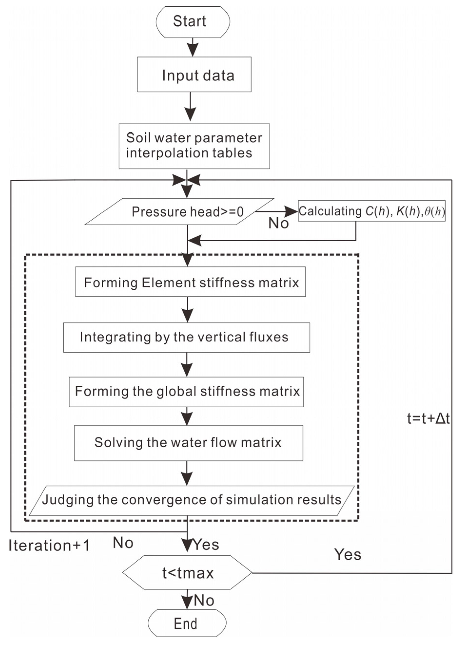
4. The Flow Chart of the Model

The model is written in FORTRAN. It runs from processing the input information, then calculating the interpolation table of the soil water parameters of θ(h), K(h) and C(h). Judgement is made on whether the nodes are in the saturated or unsaturated zone. If the nodes are in the unsaturated zone, it is necessary to calculate the soil water capacity and hydraulic conductivity according to Equations (6) and (7). Then, the model moves to form the element matrices, considering the boundary conditions. The implicit method of temporal discretization is adopted to form the unified global matrix. The global matrix is then modified with the vertical fluxes according to Equations (23)–(25). The final global matrix can be solved by solvers such as the ORTHOFEM package [30]. If the simulation results converge, the model will move to the next time step. Otherwise, the iteration will be continued in the current time step. The flow chart of the model can be seen in Figure 3.

5. Case Study

In order to test the validity, accuracy and reliability of the model code, three hypothetical cases with 1-D infiltration flow, 2-D lateral flow and 3-D well flow are implemented. Results for the hydraulic head, soil moisture content and water table contours from the proposed model are compared with the 1-D unsaturated-saturated model Hydrus1D [31], 2-D model SWMS2D [32] and 3-D model FEFLOW. Furthermore, the model is applied to a regional scale irrigation district located in Hetao irrigation district to simulate the groundwater fluctuations to assess the model applicability and efficiency. The model calibration and prediction results of water table are assessed by measurements.

5.1. Model Code Verification Cases

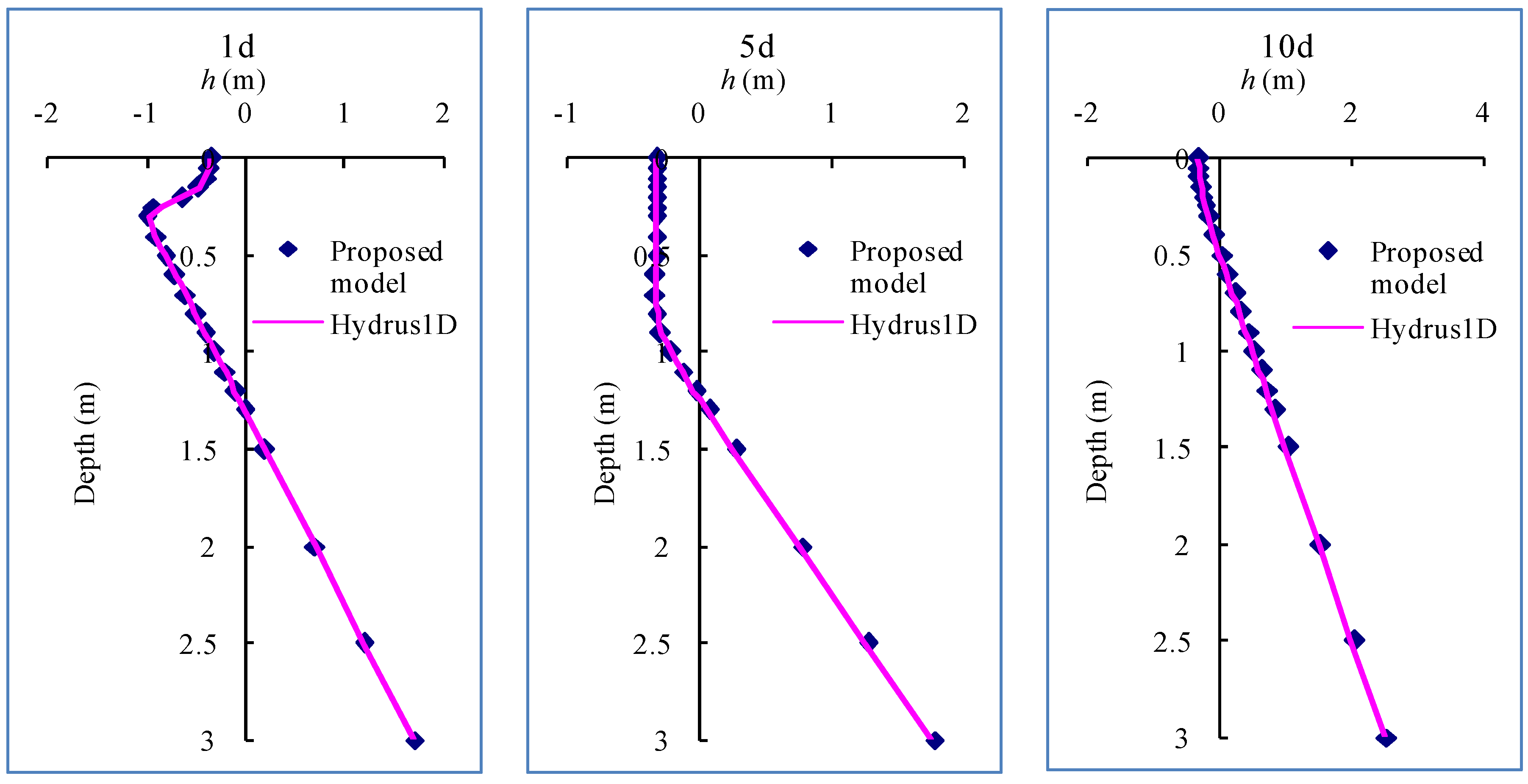
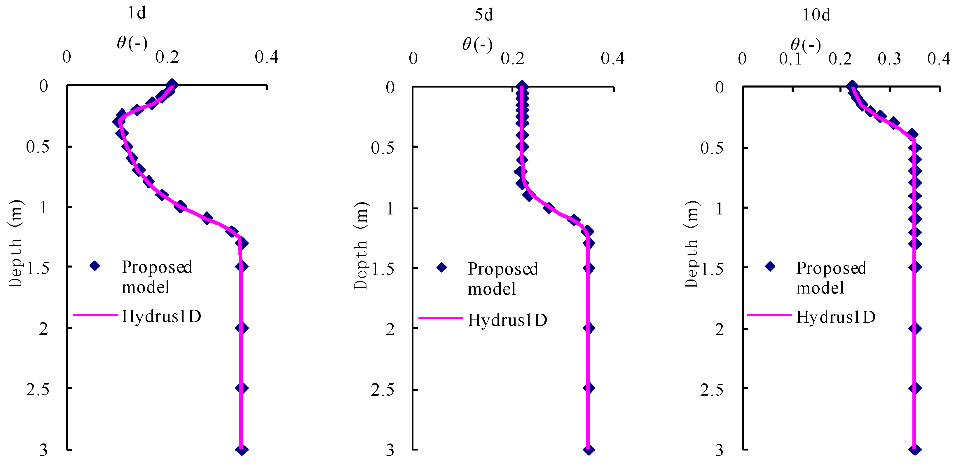
5.1.1. Case 1: 1-D Infiltration Flow

Case 1 considers 1-D infiltration water flow in a 3 m soil column, subjected to a second-kind upper boundary condition with a flux rate of 0.0005 m·d⁻¹. The soil water flow parameters are, θ_m = θ_s = 0.35, θ_r = θ_a = 0.057, K_s = 0.6 m·d⁻¹, α = 4.1 m⁻¹, n =2.28. The column bottom is prescribed as a no-flow boundary condition. The initial water table is located at a depth of 1.3 m from the soil surface. The pressure head and soil water moisture from the proposed model are compared with those from Hydrus1D, as shown in Figure 4 and Figure 5. The comparison results indicate that the absolute errors for the head are less than 0.004 m, and less than 0.0003 for soil moisture. The results indicate that the proposed model is able to precisely capture the flow information in the vertical profile.

In this case, since 3-D meshes are used in the proposed model and consequently many more nodes are calculated, the computational cost of our model is larger than that of Hydrus1D. The simulation time of the proposed model is 42 s whereas that of Hydrus1D is less than 1 s.

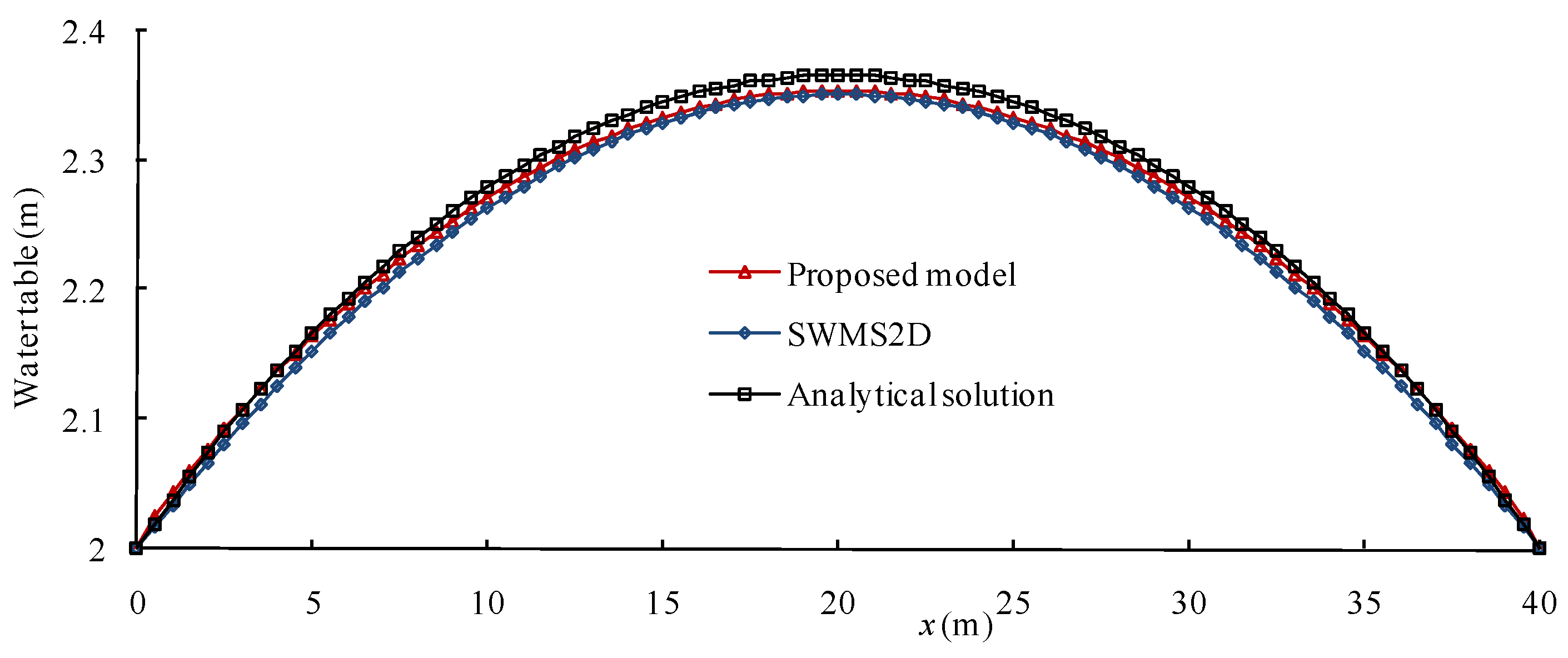
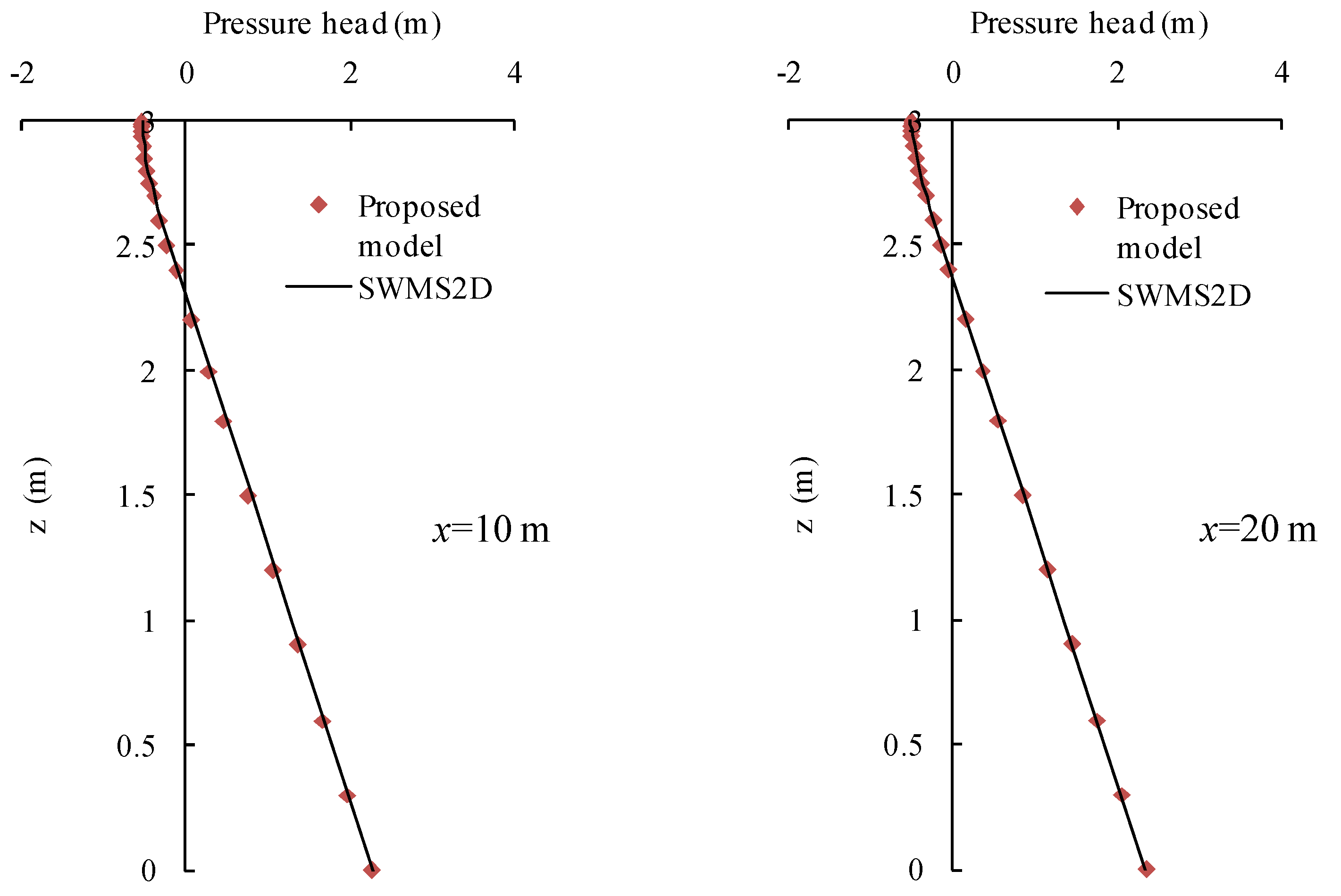
5.1.2. Case 2: 2-D Water Flow

The model is used to simulate a typical 2-D lateral flow case with two rivers 40 m apart and with precipitation infiltration from the upper boundary. The infiltration rate is 0.002 m·d⁻¹. The soil profile is homogenous and 3 m deep. The soil water parameters are θ_m = θ_s = 0.30, θ_r = θ_a = 0.02, K_s = 0.5 m·d⁻¹, α = 4.1 m⁻¹, and n = 1.964. When the water flow reaches a steady state, the analytical solution of hydraulic head for this case is given as

$$H^2=H_1^2+\frac{H_2^2-H_1^2}{l}x+\frac{W}{K_s}\left(lx-x^2\right)$$

(38)

where H is the hydraulic head at the location with a distance of x from the left river [L]; H₁ and H₂ are the constant hydraulic heads in the left and right rivers [L], respectively; l is the distance between the two rivers [L]; W is the precipitation rate [L T⁻¹]; and K_s is the saturated hydraulic conductivity [L T⁻¹].

The 2-D unsaturated-saturated model SWMS2D is also adopted to simulate this case to obtain the numerical solution. The domain is discretized into 21 layers in the simulation of the two models. The steady-state water table, where the zero location is at the bottom, i.e., z = 0 m, obtained with the proposed model, the analytical solution and SWMS2D are plotted in Figure 6. The absolute errors of the proposed model related to the analytical solution and SWMS2D are 0.0075 m and −0.0072 m, respectively. In order to check the model accuracy in the unsaturated zone, the simulated pressure head profiles at different locations are compared with those from SWMS2D as shown in Figure 7. The results show that the model can capture the water flow information in both the saturated and unsaturated zones under the lateral flow condition.

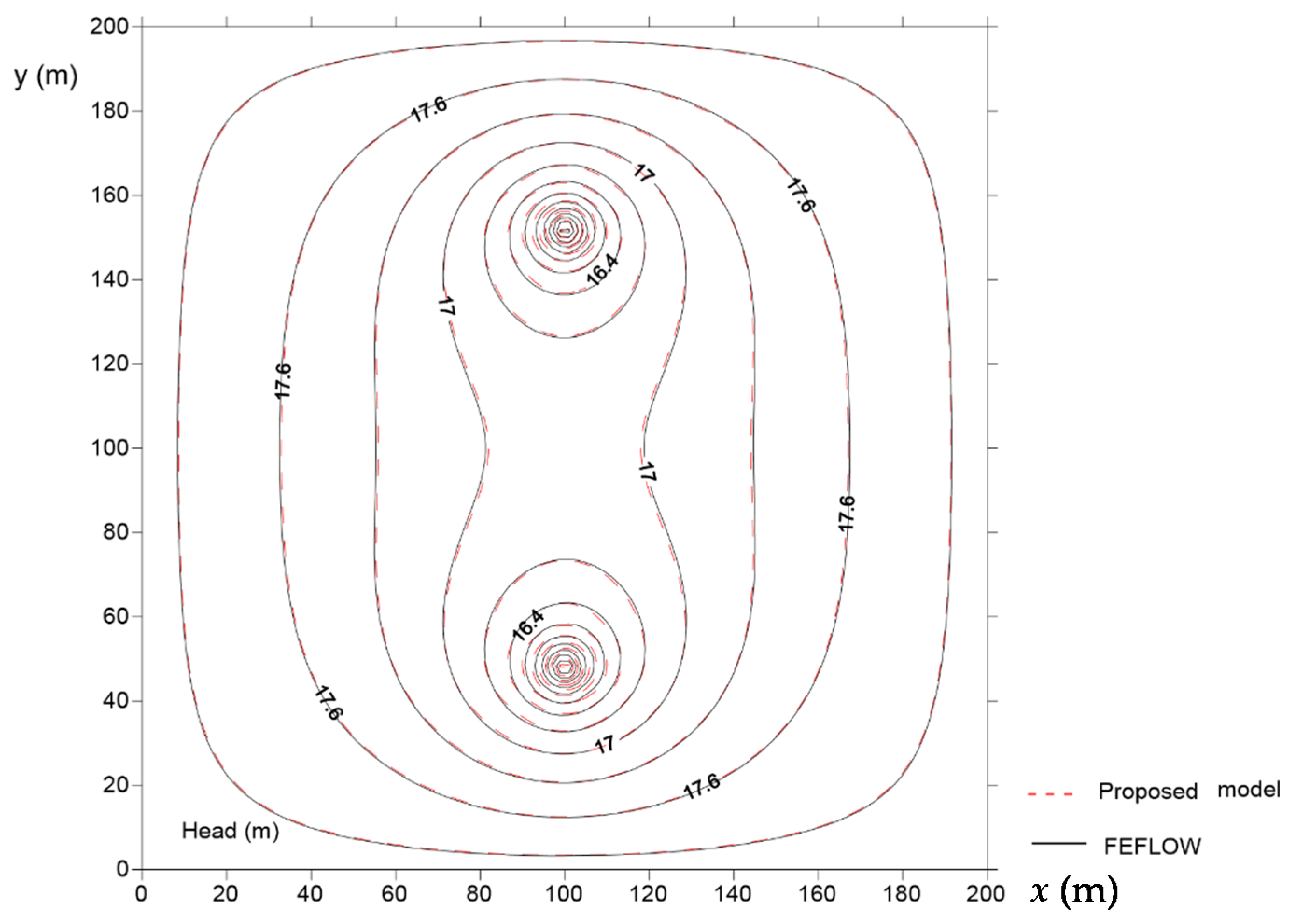
5.1.3. Case 3: 3-D Well Flow

An aquifer with the size of 200 m × 200 m × 20 m is considered. There are two pumping wells located at (100, 48) m and (100, 152) m with a pumping rate of 500 m³·d⁻¹. A constant head of 18 m is imposed around the domain, and the bottom is specified as a no-flow boundary. The water flow parameters are θ_m = θ_s = 0.30, θ_r = θ_a = 0.02, K_s = 6.4 m·d⁻¹, α = 4.1 m⁻¹, and n = 1.964. The simulation time is 200 days. The 3-D unsaturated-saturated water flow model FEFLOW is adopted to provide the reference solution. Figure 8 shows the head contours of the two models at the end of the simulation. The two head contour categories of the figure indicate that the heads of the proposed model match the solution of FEFLOW well.

In this example, the node number of the proposed model and FEFLOW are the same. The computational time is 90 s for the proposed model versus 137 s for FEFLOW, which indicates that the proposed model is efficient while still providing satisfactory simulation accuracy.

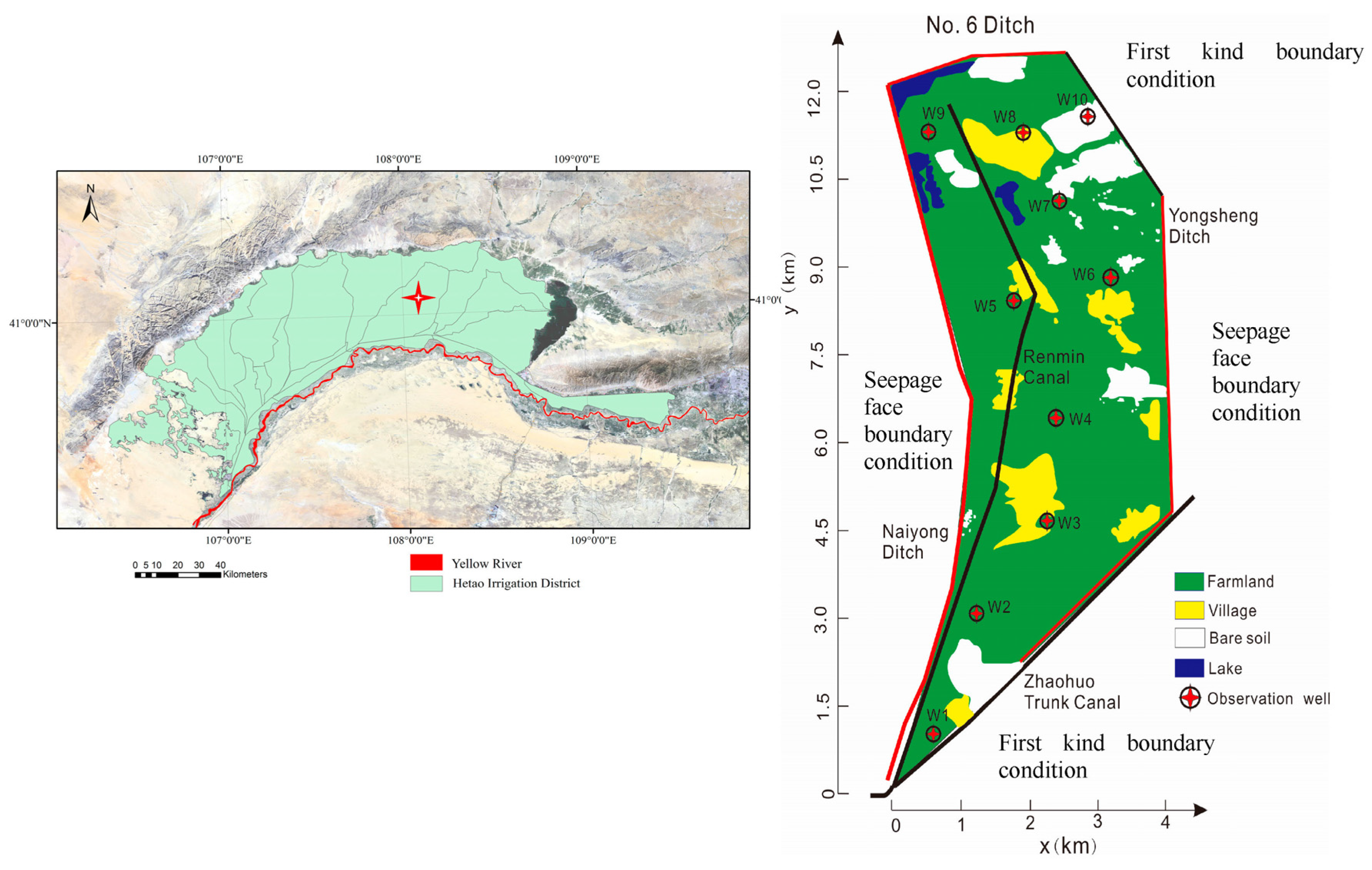
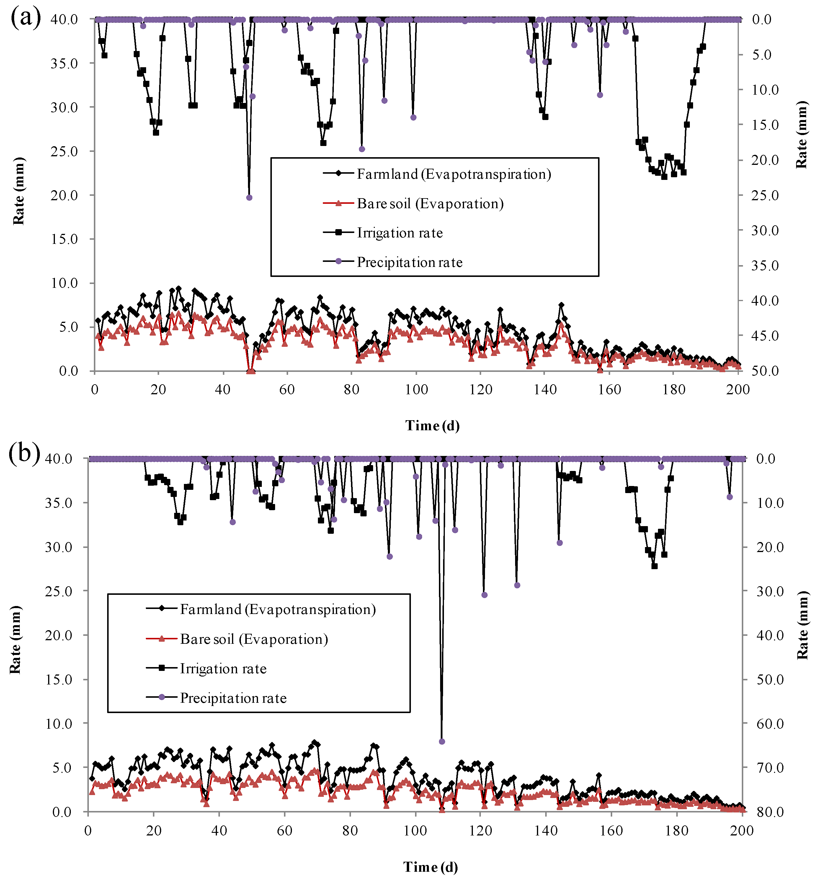
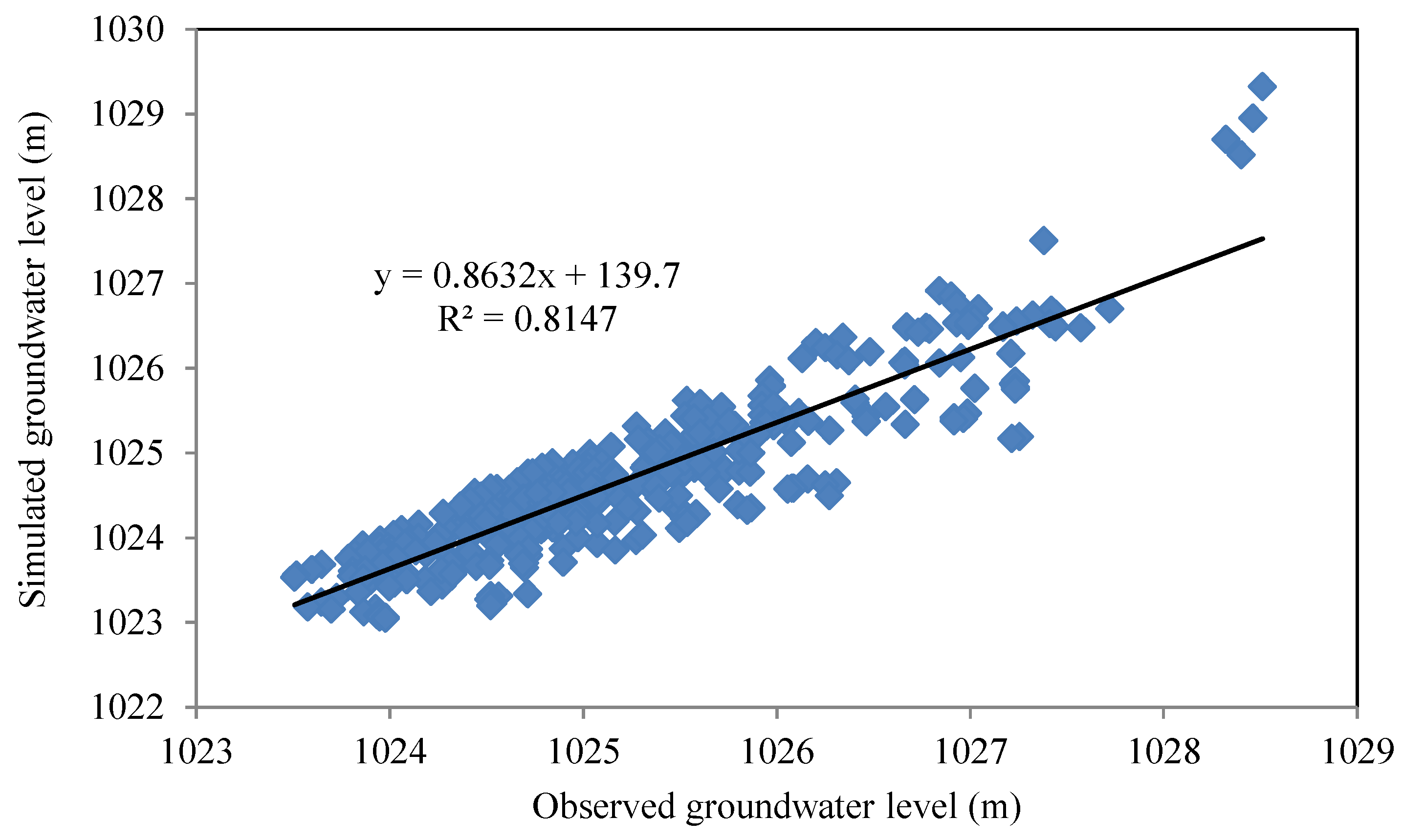
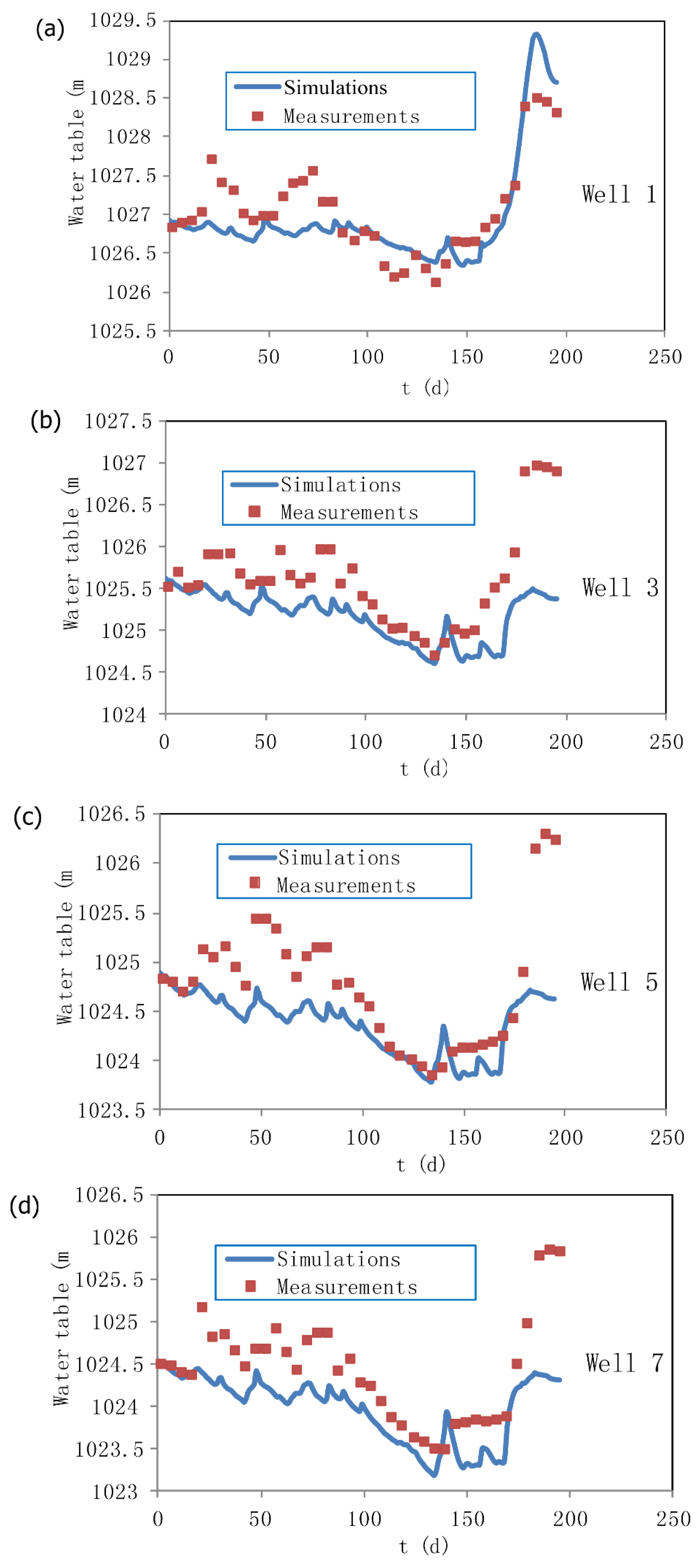
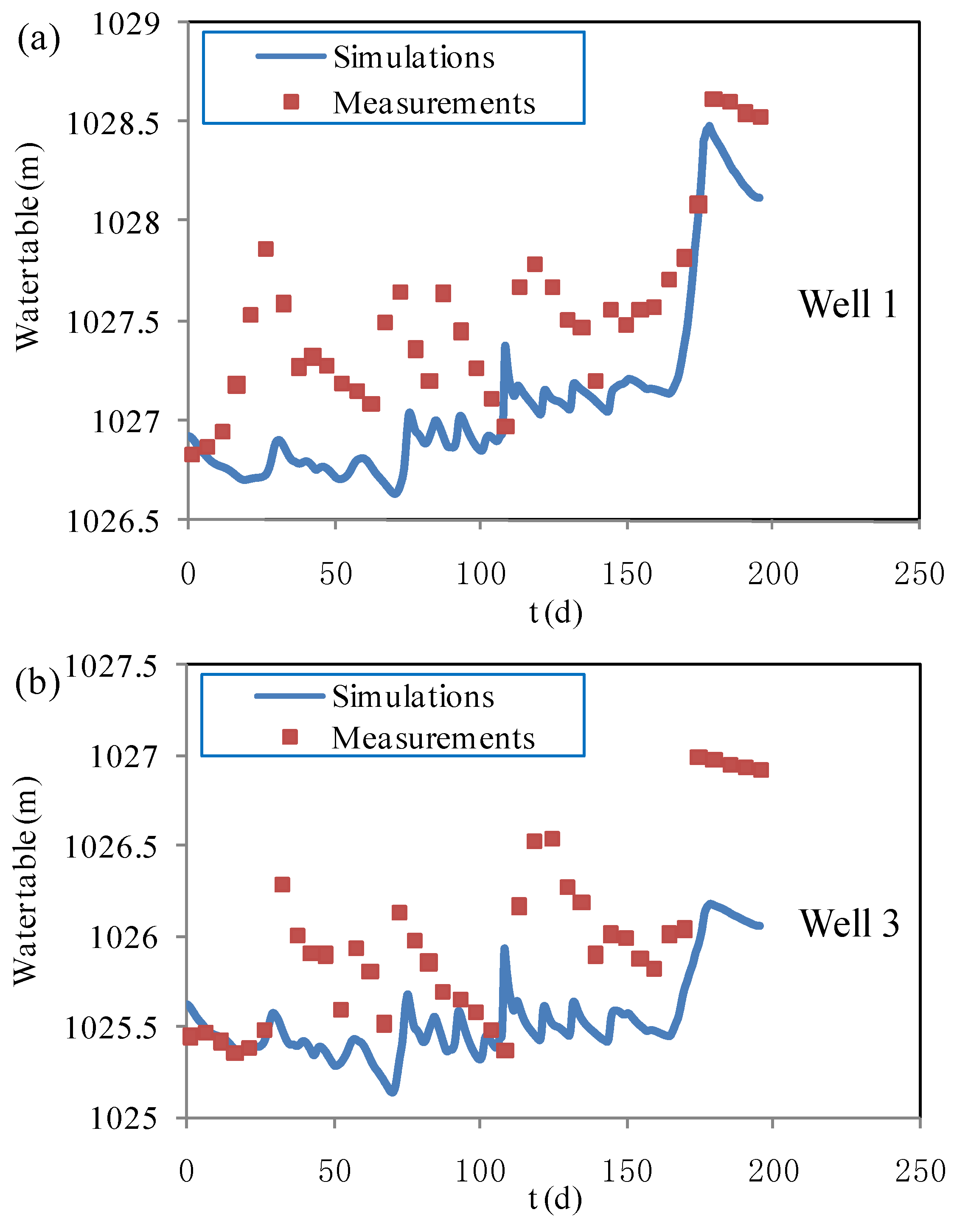
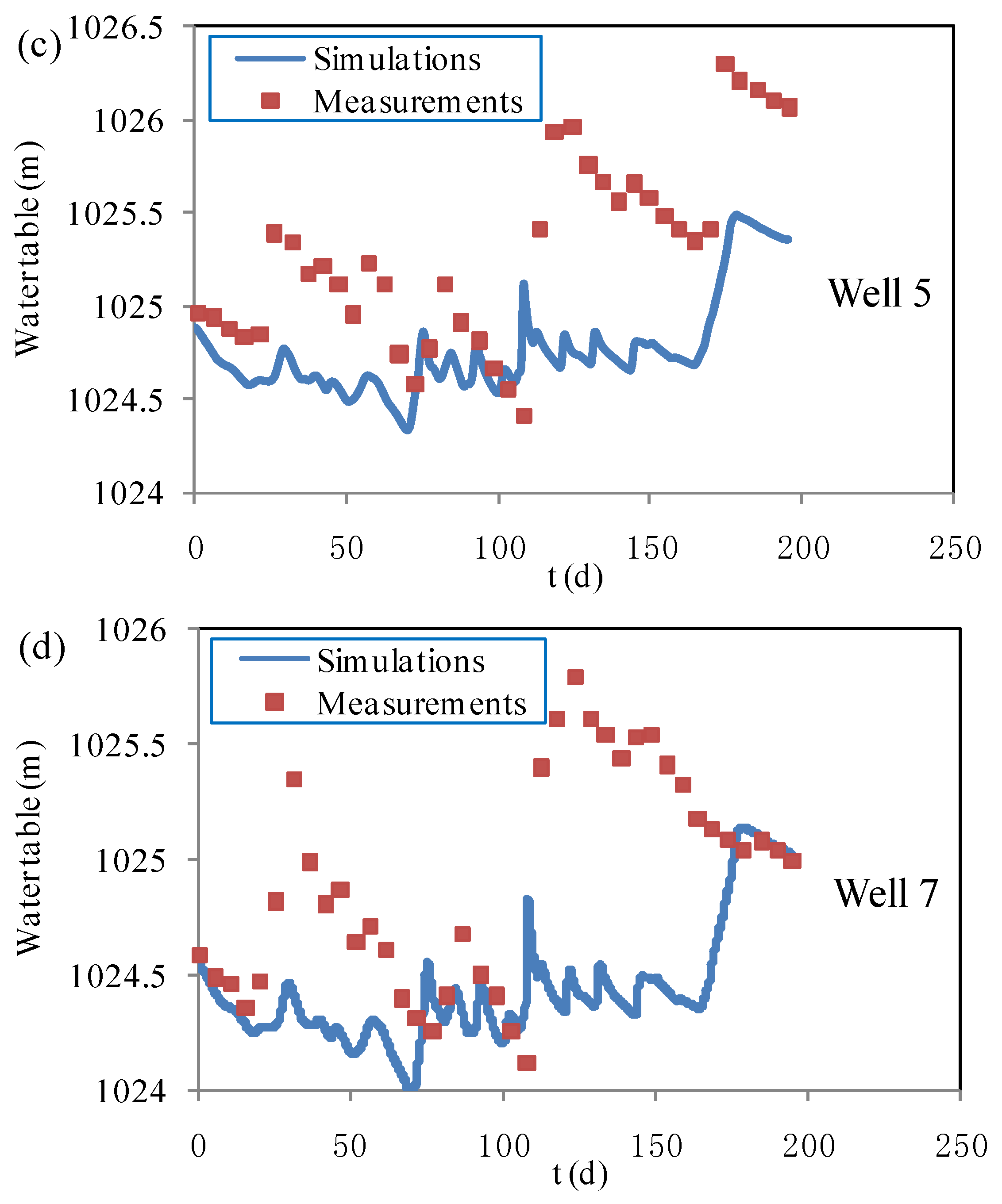
5.2. Model Application to a Regional Scale Irrigation District

After testing the validity of the proposed model, we further apply it to a regional-scale case, the Yonglian irrigation area in Hetao irrigation district, Inner Mongolia, China (Figure 9), with an area of approximately 29.1 km². The ground surface is very flat as the elevation changes only from 1028.9 m to 1025.4 m from the southwest to the northeast. This is a typical arid area with an average annual precipitation of 169 mm, but an average annual potential evaporation of 2065 mm. Therefore, irrigation is very important to ensure the water requirements of this region during the crop growing season. The irrigation and drainage canal systems clearly delineate the hydro-geological borders in this area, which are formed by the No. 6 Drainage Ditch and Yongshen Ditch in the east and the Zhaohuo Trunk Canal and Naiyong Ditch in the southwest (Figure 9).

First-kind boundary conditions are applied to these two canal segments, which are filled most of the time with irrigation or drainage water. The other segments are considered as the seepage face boundary condition. When the nodes become saturated, the pressure heads are set as zero and then the fluxes can be calculated. Otherwise, the fluxes are set as zero and the pressure heads can be calculated. The daily precipitation rate is measured in this area and the daily amount of irrigation water from Zhaohuo Trunk Canal is also measured. The irrigation rate is calculated by dividing the daily irrigation water amount diverted from Yellow river by the area of the farmland. The daily reference evapotranspiration rate is calculated by multiplying the daily evaporation from the water surface with a coefficient α, which is 0.68 in our study.

From Figure 9, it can be seen that the major land use types are farmland, bare saline soil, and villages. The assumptions here are that the area of villages is classified as bare soil, and the crop types in the farmland are not further distinguished. Therefore, the domain is divided into two sub-areas horizontally according to land use types. In each sub-area, specified upper boundary conditions (mainly with different irrigation and evaporation rates) are imposed. The details will be found in the model parameter calibration and model predictions in the following paragraphs. The aquifer geometry and hydro-geological information are obtained from the boreholes and pumping tests [33]. Provided by the Geological Department of Inner Mongolia, there is a 1-m thick impervious clay layer at the depth of 53 m from the ground surface, which is, consequently, considered as a non-flow bottom boundary in the model. Thus, the simulated aquifer has a depth of 53 m, with the top 7 m of the aquifer consisting of loamy sand with low hydraulic conductivity, and an underlying 46 m deep sand aquifer with high permeability. The whole domain is divided into 12 layers vertically and 1336 triangular prism elements in each horizontal layer to guarantee simulation accuracy.

Ten observation wells without pumping are located in this area. The water table of these 10 wells and the soil moisture contents at the soil depths of 10 cm, 30 cm, 50 cm, 70 cm, and 140 cm are measured. The water table measurements of these 10 observation wells from 1 May to 1 November 2007 are used to calibrate the model parameters. The upper boundary conditions with the precipitation in the whole domain, the irrigation rate in the farmland, the evapotranspiration in the farmland and the evaporation in the bare soil in 2007 are shown in Figure 10a. The observed water tables at the 10 observation wells on 1 May 2007 are used to interpolate the initial hydraulic head for the transient simulations.

The groundwater level data from the 10 observation wells are used to evaluate the model performance. Observed and simulated groundwater levels are compared through linear regression, and the respective coefficient of determination for the groundwater levels is 0.8147 as plotted in Figure 11. The simulated groundwater level results of the randomly selected four observation wells, which are wells 1, 3, 5, 7, are presented in Figure 12. It can be seen that the water table dynamics have a very similar trend mainly due to the intensive irrigation and evaporation rates in this area, which result in water table fluctuations occurring mainly in the vertical direction. The same soil characteristics in the horizontal direction according to the hydro-geological data also contribute to the similar water table fluctuation trend in these four locations. The results show that the model can represent the fluctuations of the observed groundwater table well. Therefore, the parameters used in the calibrated model can be considered to carry out the model prediction for the subsequent year 2008. The calibrated soil water parameters of Equations (6) and (7) are listed in

Table 1. Calibrated soil water parameters of the Yonglian irrigation area.

Depth (m)	θr (−)	θs (−)	α (m)	n (−)	Ks (m d−1)	θa (−)	θm (−)	θk (−)
0–7	0.02	0.43	2.1	1.61	1.2	0.02	0.43	0.43
7–53	0.01	0.42	2.1	1.61	5.2	0.01	0.42	0.42

.

Then, the 2007 calibrated model is applied to simulate the unsaturated-saturated water flow in 2008, with the upper boundary conditions shown in Figure 10b. The simulation runs from 1 May 2008 to 11 November 2008, lasting 195 days. Figure 13 shows the simulated and measured groundwater levels over time for the four randomly chosen wells. From Figure 13, it can be seen that the model maintains the same change trend as the observations and can capture the fluctuations of water tables. However, at simulation time t = 108 d, there is an abrupt rise in the water table observed at all observation wells, which is caused by an intensive precipitation rate (Figure 10b). The model fails to simulate this strong change in the water table, resulting in large errors in the water table at this time, as shown in Figure 13. The differences may be attributed to the high precipitation rate causing water ponding at the surface, which cannot be included in the proposed model. The uncertainties in the model parameters and model inputs as well as the setup of the boundary conditions would also affect the simulation results.

Figure 14 shows the water table distributions at two different times (t = 6 d and t = 180 d). It can be seen that the flow direction is mainly from southwest to northeast. The water table at time 180 d is higher than that of day 6 because of the large amount of irrigation water applied in the autumn season to wash out the salt in the unsaturated zone. These results demonstrate that the model works well as the variations of the hydraulic head are well simulated, even with these complicated boundary conditions and changing water supply conditions.

The computational time needed to perform the calculation is of paramount importance, because it seriously affects the model’s applicability to regional-scale problems. The domain is divided into 8760 nodes and 16030 elements. The model runs on an 8 GB RAM, eight 3.70 GHz Intel Xeon CPU–based computer, and it takes the coupling model 642 s to perform this case with 1967 time steps. Thus, the model can be considered as highly efficient to simulate a regional scale unsaturated-saturated water flow problem.

6. Conclusions

In this paper, the VHS concept is used to simplify 3-D unsaturated-saturated water flow models. This paper presents not only the theoretical basis of the VHS-based modeling but also three synthetic cases for methodology evaluation and a real world application to a regional-scale problem. The model can capture the details of water flow in both the soil zone and groundwater system as shown in the three synthetic cases, which demonstrate the accuracy of the model code. The real world application to an irrigation district with complex boundary conditions shows great applicability to complicated large-scale regional groundwater flow modeling with relatively low computational cost. It means that the VHS-based modeling has a great potential for simulating water dynamics under changing management conditions of water use reduction, which is important for water sustainability in arid and semi-arid areas [34,35].

As this study mainly focuses on the model development, the uncertainty in model calibration, various scenarios of measurements, and boundary conditions are not discussed [36]. Further, the current model treats rivers as the Dirichlet boundary condition by assigning hydraulic heads to the river nodes. However, a stream package for complex river conditions is needed. These two areas of study are warranted in a future investigation.

References

1. Kinzelbach, W.; Barer, P.; Siegfried, T.; Brunner, P. Sustainable groundwater management-Problems and scientific tools. Episodes 2003, 26, 279–284. [Google Scholar]
2. Petheram, C.; Dawes, W.; Grayson, R.; Bradford, A.; Walker, G. A sub-grid representation of groundwater discharge using a one-dimensional groundwater model. Hydrol. Process. 2003, 17, 2279–2295. [Google Scholar] [CrossRef]
3. Zhu, Y.; Shi, L.S.; Yang, J.Z.; Wu, J.W.; Mao, D.Q. Coupling methodology and application of a fully integrated model for contaminant transport in the subsurface system. J. Hydrol. 2013, 501, 56–72. [Google Scholar] [CrossRef]
4. Brunner, P. Water and Salt Management in the Yanqi Basin, China; Eidgenössische Technische Hochschule ETH: Züric, Switzerland, 2005. [Google Scholar]
5. Pikul, M.F.; Street, R.L.; Remson, I. A numerical model based on coupled one-dimensional Richards and Boussinesq equations. Water Resour. Res. 1974, 10, 295–302. [Google Scholar] [CrossRef]
6. Van Dam, J.C. Field-Scale Water Flow and Solute Transport. SWAP Model Concepts, Parameter Estimation, and Case Studies. Ph.D. Dissertation, Wageningen University, Wageningen, The Netherlands, 2000; p. 167. [Google Scholar]
7. Niswonger, R.G.; Prudic, D.E.; Regan, R.S. Documentation of the Unsaturated-Zone Flow (UZF1) Package for modeling unsaturated flow between the land surface and the water table with MODFLOW-2005; Techniques and Methods 6-A19; U.S. Geological Survey: Reston, VA, USA, 2006; p. 62.
8. Twarakavi, N.K.C.; Šimůnek, J.; Sophia, S. Evaluating interactions between groundwater and vadose zone using the HYDRUS-based flow package for MODFLOW. Vadose Zone J. 2008, 7, 757–768. [Google Scholar] [CrossRef]
9. McDonald, M.G.; Harbaugh, A.W. A Modular Three-Dimensional Finite-Difference Groundwater Flow Model; Techniques of Water-Resources Investigations of the United States Geological Survey: Reston, VA, USA, 1988.
10. Diersch, H.J.G.; Kolditz, O. Coupled groundwater flow and transport: 2. Thermohaline and 3D convection systems. Adv. Water Resour. 1998, 21, 401–425. [Google Scholar] [CrossRef]
11. Spitz, F.J.; Nicholson, R.S.; Daryll, A.P. A nested rediscretization method to improve pathline resolution by eliminating weak sinks representing wells. Ground Water 2001, 39, 778–785. [Google Scholar] [CrossRef] [PubMed]
12. Mehl, S.; Hill, M.C. Three-dimensional local grid refinement method for block-centered finite-difference groundwater models using iteratively coupled shared nodes: A new method of interpolation and analysis of errors. Adv. Water Resour. 2004, 27, 899–912. [Google Scholar] [CrossRef]
13. Di Giammarco, P.; Todini, E.; Lamberti, P. A Conservative finite elements approach to overland flow: The control volume finite element formulation. J. Hydrol. 1996, 175, 267–291. [Google Scholar] [CrossRef]
14. Zhu, Y.; Shi, L.S.; Lin, L.; Yang, J.Z.; Ye, M. A Fully Coupled Numerical Modeling for Regional Unsaturated-Saturated Water Flow. J. Hydrol. 2012, 475, 188–203. [Google Scholar] [CrossRef]
15. Sophocleus, M.; Perkins, S.P. Methodology and application of combined watershed and groundwater models in Kansas. J. Hydrol. 2000, 236, 185–201. [Google Scholar] [CrossRef]
16. SWIM—Soil and Water Integrated Model. Available online: https://www.pik-potsdam.de/research/climate-impacts-and-vulnerabilities/models/swim (accessed on 20 April 2016).
17. Facchi, A.; Ortuani, B.; Maggi, D.; Gandolfi, C. Coupled SVAT–groundwater model for water resources simulation in irrigated alluvial plains. Environ. Model. Softw. 2004, 19, 1053–1063. [Google Scholar] [CrossRef]
18. Yakirevich, A.; Weisbrod, N.; Kuznetsov, M.; Villarreyes, C.A.R.; Benavent, I.; Chavez, A.M.; Ferrando, D. Modeling the impact of solute recycling on groundwater salinization under irrigated lands: A study of the Alto Piura aquifer, Peru. J. Hydrol. 2013, 482, 25–39. [Google Scholar] [CrossRef]
19. Lardner, R.; Cekirge, H. A new algorithm for three-dimensional tidal and storm surge computations. Appl. Math. Model. 1988, 12, 471–481. [Google Scholar] [CrossRef]
20. Tsai, T.L.; Yang, J.C.; Wu, C.H. Layered and regional land subsidence model. J. Chin. Inst. Civ. Hydraul. Eng. 1998, 10, 617–626. [Google Scholar]
21. Drønen, N.; Deiggard, R. Quasi-three-dimensional modelling of the morphology of longshore bars. Coast. Eng. 2007, 54, 197–215. [Google Scholar] [CrossRef]
22. Fernando, P.T.; Pan, S. Modelling wave of hydrodynamics around a scheme of detached leaky breakwaters. In Proceeding of the 29th International Conference on Coastal Engineering, World Scientific, Lisbon, Portugal, 19–24 September 2004; pp. 830–841.
23. Li, M.; Fernando, P.T.; Pan, S.Q.; O’Connor, B.A.; Chen, D.Y. Development of a quasi-3d numerical model for sediment transport prediction in the coastal region. J. Hydro-Environ. Res. 2007, 1, 143–156. [Google Scholar] [CrossRef]
24. Lin, L.; Yang, J.Z.; Zhang, B.; Zhu, Y. A simplified numerical model of 3-D groundwater and solute transport at large scale area. J. Hydrodyn. 2010, 22, 319–328. [Google Scholar] [CrossRef]
25. Paulus, R.; Dewals, B.J.; Erpicum, S.; Pirotton, M.; Archambeau, P. Innovative modelling of 3D unsaturated flow in porous media by coupling independent models for vertical and lateral flows. J. Comput. Appl. Math. 2013, 246, 38–51. [Google Scholar] [CrossRef]
26. Van Genuchten, M.T. A closed-form equation for predicting the hydraulic conductivity of unsaturated soils. Soil Sci. Am. J. 1980, 44, 892–898. [Google Scholar] [CrossRef]
27. Zhang, W. Unsteady Groundwater Flow Calculation and Groundwater Resources Evaluation; Science Press: Beijing, China, 1983. [Google Scholar]
28. Feddes, R.A.; Kowalik, P.J.; Zaradny, H. Simulation of Field Water Use and Crop Yield; John Wiley & Sons: New York, NY, USA, 1978. [Google Scholar]
29. Doorenbos, J.; Pruitt, W.O. Guidelines for Predicting Crop Water Requirements, 24, 2nd Edition; FAO Irrigation and Drainage Paper: Rome, Italy, 1977. [Google Scholar]
30. Mendoza, C.A.; Therrien, R.; Sudicky, E.A. ORTHOFEM User’s Guide Version 1.02. Waterloo Center for Groundwater Research; University of Waterloo: Waterloo, ON, Canada, 1991. [Google Scholar]
31. Vogel, T.; Huang, K.; Zhang, R. The Hydrus Code for Simulating One-Dimensional Water Flow, Solute Transport, and Heat Movement; U.S. Salinity Laboratory Agriculture Research Service, U.S. Department of Agriculture Riverside: California, CA, USA, 1996.
32. Šimůnek, J.; Vogel, T.; van Genuchten, M.T. The SWMS_2D Code for Simulating Water Flow and Solute Transport in Two-Dimensional Variably Saturated Media, Version 1.1, Research Report No. 126; U.S. Salinity Laboratory, USDA, ARS: Riverside, CA, USA, 1992.
33. Xu, X.; Huang, G.H.; Zhan, H.B.; Qu, Z.Y.; Huang, Q.Z. Integration of SWAP and MODFLOW-2000 for modeling groundwater dynamics in shallow water table areas. J. Hydrol. 2012, 412–413, 170–181. [Google Scholar] [CrossRef]
34. Li, H.T.; Brunner, P.; Kinzelbach, W.; Li, W.P.; Dong, X.G. Calibration of a groundwater model using pattern information from remote sensing data. J. Hydrol. 2009, 377, 120–130. [Google Scholar] [CrossRef]
35. Li, H.T.; Kinzelbach, W.; Brunner, P.; Li, W.P.; Dong, X.G. Topography representation methods for improving evaporation simulation in groundwater modeling. J. Hydrol. 2008, 356, 199–208. [Google Scholar] [CrossRef]
36. Brunner, P.; Doherty, J.; Simmons, C.T. Uncertainty assessment and implications for data acquisition in support of integrated hydrologic models. Water Resour. Res. 2012, 48. [Google Scholar] [CrossRef]
Figure 1. The subsurface system and the triangular prism element as well as the horizontal plane of average head gradient in the triangular prism element.
Water 08 00195 g001
Figure 2. The water balance volume of node i. Qi means the lateral flux shown in Equation (19).
Water 08 00195 g002
Figure 3. The flow chart of the model.
Water 08 00195 g003
Figure 4. Pressure head profiles from the proposed model and Hydrus1D.
Water 08 00195 g004
Figure 5. Soil moisture profiles from the proposed model and Hydrus1D.
Water 08 00195 g005
Figure 6. Steady-state water tables obtained with the proposed model, the analytical solution and SWMS2D.
Water 08 00195 g006
Figure 7. Steady-state pressure head profiles obtained with the proposed model and SWMS2D.
Water 08 00195 g007
Figure 8. Head contours from the proposed model and FEFLOW.
Water 08 00195 g008
Figure 9. Location of the Yonglian irrigation area in Hetao irrigation district. The black border line of the Yonglian irrigation area is specified with the first-kind boundary condition, and the red border line denotes the seepage face boundary condition.
Water 08 00195 g009
Figure 10. Upper boundary conditions applied to the various sub-areas of the domain in (a) 2007 and (b) 2008.
Water 08 00195 g010
Figure 11. Comparison of observed and simulated groundwater levels for the 10 observation wells in 2007.
Water 08 00195 g011
Figure 12. Simulated and measured water table changes over time for the four selected wells, (a) Well 1; (b) Well 3; (c) Well 5; (d) Well 7, in 2007.
Water 08 00195 g012
Figure 13. Predicted groundwater table levels in 2008 compared with the measurements at (a) well 1; (b) well 3; (c) well 5; and (d) well 7.
Water 08 00195 g013aWater 08 00195 g013b
Figure 14. Simulated water table contours at times (a) t = 6 days; (b) t = 180 days.
Water 08 00195 g014