1. Introduction
In case studies, hydrological models are frequently used to compare the effects of land use, climate, or global change in different regions. One precondition for such large-scale case studies is homogeneous input data of sufficient quality regarding the model requirements. Often it is not possible to take a hydrological model developed for a specific task in a small region and apply it directly to a large region. Specific input data for large regions are not available in the same quality as for small ones, or the model has to be adjusted to specific requirements. Consequently, coarser data have to be used and models have to be simplified.
In our case, the aim was to take a wetland water balance model developed for a very specific wetland and prepare it for application to many different wetlands in a large river basin. The basis is the wetland water balance module WABI, which was developed by Dietrich
et al. [
1] as an extension for a WBalMo® model system [
2] based on the example of the Spreewald wetland (51°54′ N, 13°55′ E). The main task of the WABI module is to estimate the water demand of wetland areas as a basis for water budget calculation and water management in the WBalMo model. The integration of special modules in WBalMo model systems has often been used to integrate the requirements of different kinds of water users in this model system [
3,
4,
5].
Despite the simplifications already made compared with reality, this WBalMo Spreewald model still requires a lot of detailed data on a small scale. It contains 197 sub-areas which are treated as 197 individual water users. Thus, each wetland sub-area can get water from the river system or give water to the river system to balance its water budget in each respective month. In principle, this WABI module implemented in a WBalMo model system is applicable to any other wetland with drainage and sub-irrigation systems. However, the problem is that detailed databases of the kind available for the Spreewald wetland are not available for most wetlands. Also, the time needed to build such detailed models for a large number of wetlands is too great to build them for many wetlands in a large river basin. Because of these requirements, it is necessary to develop a simpler wetland model version based on the Spreewald model with fewer sub-areas and without violating the model assumptions, to reduce computing time, and to use consistent, commonly available data. This is the precondition for getting comparable results in regional case studies and comparing different wetlands in large river basins.
There are different tasks: (1) aggregating input data, (2) not using specific input data but instead exclusively using commonly available data, and (3) simplifying the model structure without violating the model assumptions. The literature shows many examples for coarsening the input data of models and its impact on the model results. The aggregation applies for precipitation data, soil or land use data, digital elevation models (DEMs), or spatial aggregation levels (such as sub-basins, sub-areas, parcels,
etc.). Some papers underline the effect of high-resolution precipitation data on the model results [
6,
7,
8,
9,
10]. In the case of the WBalMo Spreewald model, this is of less importance because the climate data from the next meteorological station were used and are already assumed to be homogeneous for the whole wetland. The assumption of homogeneous meteorological conditions within each wetland site is sufficient because of the size of the study sites if every wetland within a large river basis uses meteorological data from at least one unique meteorological station. Thus, the model adaptation to the regional scale focusses on aggregating the basic input parameters for soil, land use, and DEMs. Land use and the methods of coarsening land use data seem to be very sensitive parameters for the outputs of hydrological models. This also applies to changes in land use, which are part of many scenario investigations. In contrast, the enhancement of the grid size has only a small impact on the percentage of land use classes [
11,
12]. However, Becker and Braun [
13] suggest that the main land use classes should be distinguished, and [
14] found that the quality of data is more important than the spatial resolution. The level of data aggregation depends on threshold values [
15] or on the model used [
16]. This does not always have to be the case, however, as the results reported by Wegehenkel
et al. [
17] show. In a model study they found that different land use sources had only minor impacts on the simulated water balance components of evapotranspiration and groundwater recharge.
Canfield and Goodrich [
18] showed that averaging input parameter values and the geometric simplification of a model can have a minor effect on some model outputs and a major effect on others. Sivakumar [
19] underlines the need for model simplification and generalization because increasingly complex models need too much data and are often developed for specific situations. Krysanova
et al., Guntner
et al., and Chien and Mackay [
20,
21,
22] showed that the results of simple sub-models compared to complex sub-models can be sufficient in most cases, depending on the target of the model application. Besides spatial aggregation, temporal aggregation can also have an impact on the model results [
12,
23,
24,
25]. In this study, intervals of one month were the default given by the WBalMo model system. Other intervals were not considered.
This paper describes how the WABI module was simplified, turning it from a module for a single wetland model to a module for a large-scale model system. The specific detailed database was adjusted to use commonly available data and to be based on comparable basics on a large scale. The database of the WBalMo Spreewald model was adapted to use commonly available data and coarsened step by step. Then a method was developed to aggregate small sub-areas into larger units without violating various model constraints. The impact of the different aggregation and simplification steps on the main model outputs are compared and discussed in the results. Different kinds of input data and model structure are used to show their effects on the results, the applicability, and the constraints of modeling at the regional scale.
2. Materials and Methods
2.1. Test and Application Area
The Spreewald wetland is situated 70 km south-east of Berlin in the Spree River basin (
Figure 1). The area of the wetland is about 320 km
2. Land use is mainly grassland, arable fields, and forests. The soils are dominated by gleyic sands and fens. A detailed description of the wetland and the water resource management systems in the wetland and its sub-basins is given by Dietrich, Redetzky, and Schwärzel [
1]. The wetland was used to develop a simplified version of the WBalMo Spreewald model.
The application area for the simplified model is the Elbe Lowland in the northern part of the Elbe River basin (148,000 km
2) in Germany. Thirty-five wetlands larger than 1000 ha with an overall area of 3840 km
2 were selected within the Elbe Lowland for integration into the water balance model WBalMo GLOWA-Elbe [
26].
2.2. Basic Models: WBalMo, WABI, and WBalMo Spreewald I
The WBalMo model system [
2,
27] served as the basis for the Elbe basin study in the GLOWA-Elbe research project ([
28]). This system simulates both hydrological processes and water management in a river basin. River basins are represented by simulated sub-basins, stream networks, balance profiles, water users, and reservoirs. The input variables are time series, either calculated using precipitation runoff models or generated stochastically. Water use processes, such as the management of reservoirs or water extraction by power plants, are reproduced by deterministic means [
29]. The time step is one month. The specific module WABI was integrated into WBalMo to calculate the water balance of the groundwater-influenced areas with drainage and sub-irrigation systems. To use this module, a wetland was divided into sub-areas: the smallest areas where the groundwater level could be regulated separately. Two important assumptions regarding the WABI module are that the groundwater surface in each sub-area can be approximated as a horizontal plane, and that the water distribution and exchange within the wetland will be realized entirely by the channel network. Only sub-areas at the border of the wetland can be supplied from the surrounding aquifer. The module requires monthly target groundwater levels for each sub-area, and information about the frequency distribution of elevation values, land use, and soil types, as well as a storativity function extended for open water conditions. Further, it takes into account precipitation and potential evapotranspiration, and data for target groundwater levels. It provides the actual evapotranspiration, the discharge into the channel network or directly into the river, and the groundwater level in each sub-area. A detailed description is given in Dietrich, Redetzky, and Schwärzel [
1] of the basic models, how the WABI module is integrated into the WBalMo system, and the model tests using the example of the Spreewald wetland.
The original Spreewald model, called WBalMo Spreewald I here, contains 135 streams with 89 nodes with defined water distributions. The wetland area (320 km2) is divided into 197 sub-areas. Each of the sub-areas is regarded as a separate water user in the model. The database (DEMs, soil map, land use map) consists of particularly detailed data not available for all wetlands in the Elbe Lowland. In consequence, it was necessary to adjust the WBalMo Spreewald I model, turning it into a database which was available for the whole Elbe Lowland, and to simplify the model for use on a larger scale, before assembling the wetland models for all 35 selected wetlands.
2.3. Adaptation of the Basic Model to the Scale of the Whole Elbe Basin
The adaptation of the basic model to the scale of the whole Elbe basin was carried out in two steps. The basis is the model WBalMo Spreewald I. In the first step the database of this model was gradually modified and simplified. This work was done in the pre-processing: different variants of input data were calculated with the existing model and selected results were compared. It was not our ambition to develop all the variants which can be created by combining the different input parameters. Our approach was to start the simplification with one parameter and to find the level which had no relevant impact on the results. Then this parameter was fixed and the next parameter was modified in the same way, and so on. Thus the number of variants was manageable, but also incomplete from the point of view of combinatorial analyses. However, it is not possible to compare the impact of each parameter with the impact of every other parameter.
In the second step the model structure was simplified by collating sub-areas of the wetland into larger sections. Both steps are described in detail in the following.
2.4. Adaptation of the Database
The model WBalMo Spreewald I was developed based on specific, detailed data:
DEM: DEM10, a combination of a laser scan DEM [
30] and a DEM based on digitized topographic maps at a scale of 1:10000 [
31],
digital land use maps: BTSPW (Spreewald biotope type mapping [
32]) with seven land use classes,
digital soil map: BÜK300 [
33] with five soil types.
Mainly, such detailed data are only available for the Spreewald wetland or a few selected other wetlands. Comparable data available for the whole state of Brandenburg and all the other federal states of Germany are:
digital land use map: BTBRB (Brandenburg biotope type mapping [
35]),
digital land use map: CORINE land cover [
36],
digital soil map: BÜK300 [
33].
The grid size of the entire digital database used is 25 m × 25 m.
During the scaling procedure one database was either exchanged or modified as the number of classes was reduced. The number of soil classes in BÜK300 was reduced step by step from five to one (
Figure 2) and all other parameters remain the same (variants 0 to 3). Then the soil map with four soil classes (BÜK300/4) was used for the variants where the other parameters were modified.
The number of land use classes on the BTSPW map was reduced from seven to four (
Figure 3). The class “intensive grassland” was changed to “extensive grassland”, while the classes of urban and unused land were integrated into the land use classes of their surrounding areas. The land use maps were combined with the soil map with four classes and the DEM10. Than the BTSPW land use map was exchanged with the BTBRB map and CORINE map. Both maps distinguish between four land use classes.
Two different DEMs were used. The differences between these DEMs are relatively minor for the whole wetland (
Figure 4). In the variants, at first the DEM10 was combined with the soil map and the land use maps (variants 0 to 6). In variant 7, the DEM25 was combined with the soil map with four classes as well as the BTBRB with four classes.
Table 1 describes the soil/land use/DEM combinations of the variants.
After each step the soil map and the land use map were intersected in the GIS (geographic information system). The results are hydrological response units, from which the input values were produced for the WBalMo Spreewald model. The storage curves of the sub-areas were calculated along with the DEM. All parameter sets necessary for the WBalMo Spreewald model are described in Dietrich, Redetzky, and Schwärzel [
1]. Subsequently, the model was run for all variants using the same meteorological and hydrological time series from 1990 to 2000. The monthly target water levels were always the same for each year and all variants.
2.5. Adaptation of the Model Structure
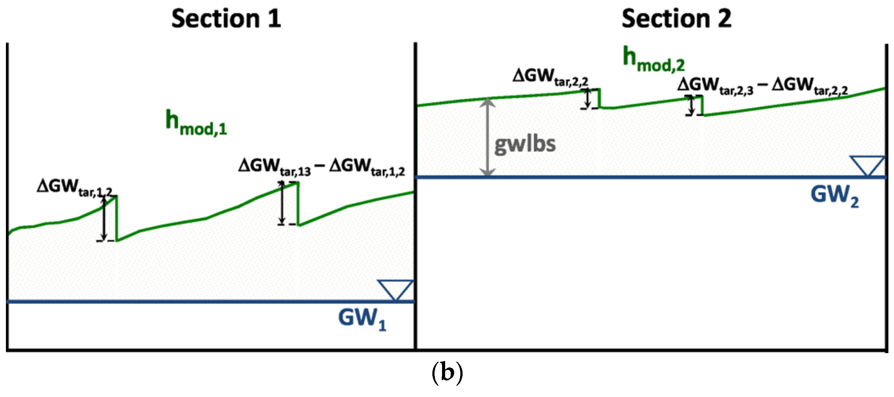
The model structure of the detailed model WBalMo Spreewald I was adapted to the larger scale. Smaller sub-areas of the wetland were aggregated to form larger sections. This reduces the number of water users in the model as well as the number of distribution nodes, meaning that the model run time was shortened. This aggregation is possible because in practice several weirs are often regulated in groups or only the main weirs are regulated, not each of the smaller weirs. The only problem with this aggregation is fulfilling the model assumption of a horizontal plane groundwater level in a sub-area despite the larger units. The relief can be more heterogeneous or there can be a slope in the groundwater surface at the edge of the wetland. Normally, a sufficient reproduction of the real groundwater levels below the surface is only possible if the sub-areas are not too large, especially for difficult hydrological conditions. As this is a precondition for accurately calculating the evapotranspiration, this problem was solved by modifying the DEM (
Figure 5). In the modified DEM the relations between the smaller sub-areas were considered in the new sub-areas, here called sections. The following procedure was adopted:
“Sub-areas” (
sub) describes a set of properties such as area (
A), target water levels (
GWtar), and surface elevations (
h)
Sub-areas (subscript
i) were merged into new sections (
sec, subscript
j).
The target water level of the new section (
GWtar,j) is the lowest target water level of all merged sub-areas.
The difference
ΔGWtar,j,i is calculated between the winter target water level
GWtar,j and the winter target water level of each sub-area of a section (
GWtar,j,i)
Then the modified DEM
hmod,j,i is calculated by the difference between the
hj,i and
ΔGWtar,j,i and merged to
hmod,j of the new section.
The result is a modified DEM (
hmod,j) which does not have a real elevation. However, if the groundwater levels below the surface are calculated with a horizontal groundwater level for the whole section (
GWj), we get the same distribution of groundwater levels below the surface as for smaller sub-areas.
Figure 5 illustrates the procedure and the result. The upper scheme shows the initial situation for six sub-areas as an example. These sub-areas were merged to form two sections. For each sub-area a horizontal groundwater level is assumed which corresponds to the water level at the respective weir (
GWj,i). The differences between the surface elevation and the horizontal groundwater level result in a distribution of groundwater levels below the surface (gwlbs). The lower scheme shows the result of the modification of the DEM. The surface is different to the original surface. Now each of the two sections has one horizontal groundwater level (
GWj). The difference between the modified DEM and these two levels results in the same distribution of groundwater levels below the surface as in the upper scheme. The integrated larger sections with the assumption of a horizontal groundwater level in each section in our model have the same distribution of groundwater levels below the surface in the model calculations.
Simplifying the model structure results in a reduction in the number of water users from 197 (sub-areas) to 49 (sections) for the Spreewald wetland (
Figure 6). One hundred and ninety and 42 water users, respectively, are sites with groundwater levels near the surface (grassland, arable land, forest) and seven water users are fish ponds. The fish ponds are identical in both models. The size of the 190 sub-areas ranges between 19 and 648 ha. The size of the 42 sections ranges between 42 and 3300 ha. Each of the 197 sub-areas is a water user in the model WBalMo Spreewald I, and each of the new sections is a water user in the model WBalMo Spreewald II. The stream network of the model was reduced from 135 (WBalMo Spreewald I) to 50 streams (WBalMo Spreewald II), with 21 nodes with water distribution rules instead of 89 rules in WBalMo Spreewald I (
Figure 6). The model WBalMo Spreewald II was run with the same time series (1990 to 2000) as the model WBalMo Spreewald I described above.
2.6. Model Evaluation
Depending on the model's purpose, two aspects have to be considered during the model evaluation process. The first aspect is the effect of the whole wetland within the river basin. In our case the model has to work as a sub-model in a large water balance model for the whole Elbe River basin and has to calculate the water balance of large wetlands. This means the water balance of the wetland as a whole has to be reflected correctly. The best parameter to evaluate this is the difference between the discharge in the main river downstream of the wetland Rout and all inflows to the wetland Rin (Rout-Rin). In principle, this is the water withdrawal of the wetland sub-areas from the stream system, and the drainage from the wetland sub-areas to the stream system, depending on the current water balance situation.
The second aspect is correctly reflecting the hydrological behavior within the wetland. Because the wetland is divided into many sub-areas (which can be seen as sub-basins) the results for each sub-area have to be compared with the results for the corresponding sub-area of variant 0 for each time step. The most interesting factors for the scope of the model are the water balance components of evapotranspiration (
Eta), water withdrawal from the stream system (
Rw), and drainage to the stream system (
Rd), as well as the differences between the target and actual groundwater level, which is referred to here as the groundwater level deficit (
GWdef). The results of the different model variants are compared with the values of variant 0. The evaluation of variant 0 with measured discharge values and groundwater levels for selected sub-areas was described in [
1]. All variants were run with the same mathematical model. To compare the results of the aggregated model (variant 8) with variant 0, the results of the 197 sub-areas of variant 0 were aggregated to form the 49 sections of model WBalMo Spreewald II in a post-processing step.
In line with Bennett
et al. [
37] we used a mix of visual analyses and selected performance criteria to assess the model performance of the variants. The strengths and weaknesses of different criteria have been discussed in detail in different papers [
37,
38,
39]. On this basis we decided to use the standard statistics of mean and variance to compare the mean monthly values of the whole wetland. Using a simple linear regression for visual performance analyses, the root mean square error (RMSE), the standard deviation of the residue (σ
res), the Pearson coefficient of determination (r
2), and the Nash-Sutcliffe Efficiency (NSE) as the selected performance criteria, the individual values of the sub-areas and sections were each evaluated. All metrics were calculated using the equations described in Bennett
et al. [
37].
3. Results
3.1. Storage Curves
One important input parameter of the WABI module is the storage curve of each water user. The storage curves are results of the pre-processing procedure and depend on the soil parameters, the DEMs, and the partition of the wetland into sub-areas [
1]. In
Figure 7 the change in the water storage was calculated for each sub-area for a change in the groundwater levels between the minimum elevation level
Hmin of each sub-area (here set to 0 m) and 1 m below
Hmin, as well as between 1 m and 2 m below
Hmin. The figures are summarized for the whole wetland and the differences to the corresponding values of variant 0 are shown. The differences between five and four soil classes and between the variants with the two soil classes of “peat” and “sand” are minor if the DEM and the model structure are the same (±10 mm). Substituting “peat” for “sand” (variant 3) causes the whole wetland to store less water. Using DEM25 in place of DEM10 affects the storage characteristics of the range near the surface (0 to 1 m below
Hmin) more than it affects the characteristics of the range between 1 and 2 m below
Hmin. Simplifying the model by collating sub-areas has the largest effect on the storage behavior of the wetland, especially for groundwater levels near the surface. The difference between variants 0 and 8 can be up to −77 mm for the first meter.
3.2. Mean Monthly Values
Table 2 summarizes the mean monthly values of
Rout-Rin, as well as the mean monthly sum of
Eta,
Rw and
Rd of the whole wetland and the mean
GWdef of all sub-areas for all variants. There is relatively little difference in the mean values between the variants. The maximum difference between
Rout-
Rin of variants 0 and 8 is only 0.22 m
3/s. The variances for all parameters are comparatively large despite the variances for
GWdef. What is responsible for the large variances is the large fluctuations within the years, as well as differences between the years. The variance of
GWdef is small compared to its mean value and different to the variances of the other parameters because the water availability is usually enough, not least because of the target water level's adaptation to the annual cycle.
Eta, Rw, and Rd were affected by all input data (soil, land use, DEM, and model simplification). Variant 6 with CORINE land use has the lowest variance of the evapotranspiration values. The mean values of Rw and Rd are lower for the variant of the reduced model (variant 8). Whereas the variance of Rw for variant 8 is the lowest of all variants, Rd of this variant has the largest variance of all variants. The mean GWdef is the lowest for variant 8.
3.3. Monthly Water Withdrawal and Drainage of the Whole Wetland
The monthly values of
Rw and
Rd of the whole wetland show large fluctuations within every year (
Figure 8). Negative values mean that the discharge downstream of the wetland is smaller than the sum of all inflows because the water withdrawal of all sub-areas from the stream system is larger than the sum of all drainage into the stream system. In most cases this happens during the summer months, when there is high withdrawal from the wetland areas. Drainage situations are more typical for the winter months, a possible exception being months with above-average precipitation values. In such wet months, drainage can also arise in spring or summer. All variants reflect the behavior of variant 0. Variant 8 has slightly higher drainage values in some months, resulting in the higher variance value in
Table 2.
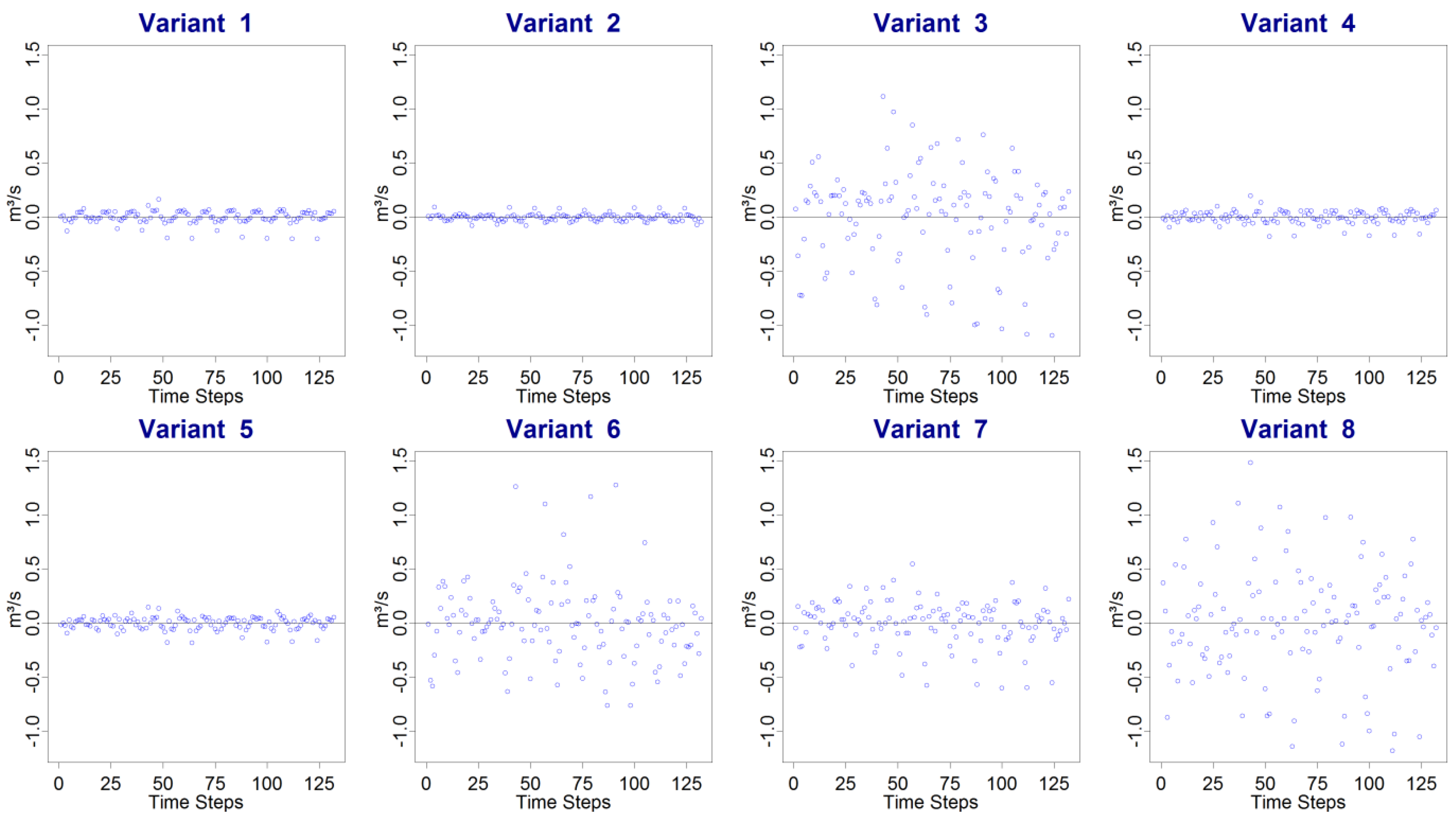
However, the differences are relatively small compared to the absolute values of discharge downstream of the wetland. The NSE and the r
2 are always nearly 1 (
Table 3). The RMSE and the σ
res show some differences between the variants. The values for variants 3, 6, and 8 are around a decimal place higher than for the other variants with the smaller changes in the database (variants 1, 2, 4, and 5). The residues of the monthly discharge values underline this (
Figure 9). They emphasize the differences between the variants, but do not show any clear patterns between the variants.
3.4. Monthly Water Balance Components within the Wetland
A summary of all the efficiency parameters for the variants of each modelled water balance component is listed in
Table 4. Generally, the model results show the best agreement for evapotranspiration. Variant 6 has the lowest NSE and r
2, and the highest RMSE of all variants. The water withdrawal of the sub-areas behaves similarly to the evapotranspiration. Only variant 3, the strongest simplification of the soil input data, also has lower values for NSE and r
2, as well as higher values of RMSE and σ
res compared to the other variants. The modelled values of the drainage from the sub-areas behave differently to those for evapotranspiration and water withdrawal. The drainage component of variant 8 has the lowest efficiency values of all four components. The soil simplification also has a higher impact than changing the land use map, as can be seen from a comparison of variants 3 and 6, though it affects drainage less than it does water withdrawal. The groundwater deficit has the largest differences between variants combined with the lowest efficiency values. Simplifying the model structure has the greatest effect on this component.
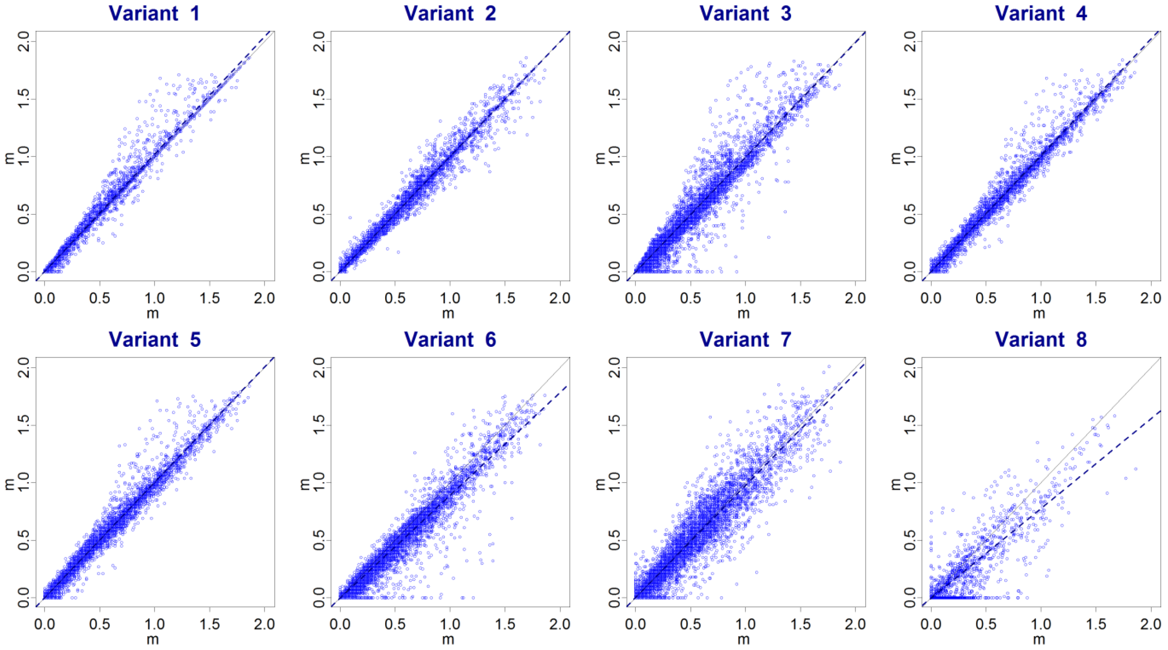
Figure 10 illustrates how the evapotranspiration values scatter increasingly as the model input data and model structure are simplified. Reducing the soil classes with low percentage (variants 1 and 2) has less impact than reducing land use classes with low percentage (variants 1, 4, and 5) if the two major soil classes of “sand” and “peat” or the major land use classes of grassland, arable land, and forest are conserved. The largest results scatter was caused by the CORINE land use map (variant 6), the DEM25 (variant 7), and by simplifying the model structure (variant 8). The linear regression models of all the variants show that although their average behavior is very similar, they differ significantly from the original model, variant 0 (level of significance 0.001). The same results were obtained for the other water balance components.
All water balance components affect the modeled groundwater levels in the wetland areas. The modifications to the soil data and the DEMs affect the water storage of the sub-areas, which represents the correlation between the water balance and the change in the groundwater levels during a model time step. The land use variants have a greater impact on the evapotranspiration, and thus the water demand, water withdrawal, and drainage of the sub-areas. The step-by-step coarsening of all input parameters (variants 1 to 8) results in an increasing scatter of the monthly groundwater deficits (
Figure 11). The largest shift of all variants with respect to variant 0 can be seen in the model featuring the CORINE land use (variant 6), while variant 8 has the largest standard deviation of the residuals. Simplifying the model structure has a greater effect on the modeled groundwater levels than on the other water balance components considered (evapotranspiration, water withdrawal, and drainage), as shown before.
4. Discussion
The main reason for using alternative input data for soil, land use, and DEMs was their availability in the whole Elbe River basin. The main aim of reducing the soil and land use classes was to reduce the number of hydrological response units, and thus to reduce the model computing time. The basic idea of the reduction steps was to add classes occurring over a small areal percentage of the whole area to include areas with a high areal percentage and nearly the same characteristics. Thus, it is not surprising that collating “loam above sand” and “loamy sand” with “sand” does not have a major effect on the water storage characteristics of the whole wetland and the calculated hydrological parameters. However, it makes a difference if we treat peaty areas like sandy areas. The water storage characteristics of the two soil types are different, and because the peaty soils make up one third of the whole area it has an impact on the water storage of the whole wetland. This affects the water demand of the wetland areas in times when the evapotranspiration exceeds the precipitation and therefore the water withdrawal from the streams. The usable water storage of sandy soils is lower than that of peaty soils, so the water withdrawal increases if water is available in the streams. In times with a water surplus in the wetland areas we have the opposite effect. Less water is stored in the wetland areas, and more water recharges into the streams. While the water withdrawal from the streams is mainly important from May to September, drainage into the streams occurs in winter and early spring. Thus, soil data coarsening affects the water balance components throughout the year. Finally, the soil simplification causes an increasing variation in the modeled discharge downstream of the wetland.
Reducing the land use classes of the detailed land use map for the Spreewald biosphere reserve (BTSPW) from seven to four has only a minor effect on the calculated evapotranspiration values because of the small areal percentage of the classes affected. Also, swapping the BTSPW map with the BTBRB one (which has four classes) results in approximate values for all calculated parameters. This is comparable with the results reported by [
11], who concluded that generalizing land cover maps showed relatively minor differences in the outflow of a modeled basin in Canada. Only the application of the CORINE land use map clearly leads to less evapotranspiration because there is a higher percentage of the arable land use class (
Figure 3) and the water withdrawal values deviate further from the zero variant. This matches the results of Bormann
et al. [
14] showing that accuracy of land use data sets is more important than a high spatial resolution. Branger
et al. [
40] also conclude that land use maps should be selected and processed with care and with specific respect to the objectives of a study. So the recommendation for land use maps in wetland areas is to employ a land use map on the basis of biotope-type mapping.
The selected DEM has an impact on the water storage characteristics of the sub-areas if groundwater levels are near the surface. If the model is used for scenarios with higher target water levels than in this paper, for example, rewetting scenarios, the importance of the DEM increases, while it decreases for deeper target groundwater levels. The scattering of all parameters is larger for the DEM25 variants than for the equal variants with DEM10. The main reason is the smaller water storage. Thus, we get larger fluctuations of the groundwater levels with an impact on evapotranspiration, as well as on water withdrawal and drainage.
The last step of the model adaptation was to simplify the model structure by collating sub-areas into sections and reducing the stream network. If we look at the results for the individual sub-areas within the wetland, they show that the last step has a greater impact on the model results than the steps of data reduction or data exchange. This confirms the relevance of the dominant processes which should be considered as best as possible in the model simplification [
19,
41]. In particular, the values of the water withdrawal decrease and the scatter of the groundwater deficit values increases. The reasons are the larger sub-areas in the simplified variants and the reduced stream network. Individual sections store more water because of the larger areas and there are fewer nodes in the stream network with rules for water distribution. Thus, the problem of the distribution of the water supply was simplified and the values for the water extraction were equalized. The variants with the simplified model also show lower groundwater deficit values for the whole wetland (
Table 2). This is also because of the balancing effect of the larger sub-areas. However, it means that individual hotspots cannot be considered, which should be the case for specific investigations within a wetland. General conclusions concerning the behavior of the whole wetland are not affected by this balancing effect of the larger sub-areas. If we evaluate the summarized results for the whole wetland, the effect of the simplification is relatively low compared to the nuanced view within the wetland. Lorite, Mateos, and Fereres [
25] found similar effects for the assessment of the irrigation requirement for different spatial aggregation levels of a 7000 ha irrigation scheme in Spain.
The results show that changing the input data and simplifying the model structure has an acceptable effect on the mean water balance components of the whole area. The mean water deficit of the whole wetland (difference between outflow and inflow) decreases slightly; the variance is nearly the same as in the base variant. The mean evapotranspiration and water withdrawal values from the streams are also slightly smaller, including their variances (
Table 2). This is because there are fewer, larger hydrological response units, which leads to simplification within the wetland. Similar effects were found by Sulis
et al. [
42] for different resolutions of DEM and responses of a hydrological model. Another aspect is the larger usable water storage obtained by modifying the DEM, especially for variant 8 (
Figure 7). Taking into account all modifications of the input values and the model structure, the lower water budget deficit results in a lower groundwater deficit.
The visual analysis of the residuals of the monthly discharge values downstream of the wetland suggests that some variants increasingly deviate from the zero variants. However, not all efficiency parameters reflect this. R
2 and NSE are constant for all variants, and only RMSE and σ
res have higher values for variants 3, 6, and 8 (one decimal place). This underlines the necessity to use different efficiency parameters for the model evaluation as recommended by Bennett
et al. [
37], Krause, Boyle, and Bäse [
38], or Moriasi
et al. [
39]. On the other hand, 90% of the relative residuals of the discharge downstream of the wetland are smaller than 5%.
If the model is to be used in large river basins, its structure has to be simplified. Nevertheless, the input data should be coarsened carefully. It is also clear that one requirement for a large-scale impact assessment in a large basin is a comparable database for the whole basin, although the accuracy requirements also have to be fulfilled.
5. Conclusions
The aim of this paper was to simplify the detailed water balance model WBalMo Spreewald I, developed for a wetland with an intensive water management system on the basis of specific input data for soil, land use, and DEMs. The simplified model was to be applied in a large water balance model for the whole Elbe River basin. Therefore, the detailed model was coarsened to create a model using commonly available data as an input, and with a simpler structure. In the different steps we replaced the specific data with commonly available data and reduced the details of the model input data. The time step was always the same. The model results of the different generalization steps were compared in visual analyses and with different efficiency parameters for the most interesting water balance components of the wetland.
The results show that soil or land use classes should only be collated for classes with low occurrence in the whole area. This reduces the amount of input data and the model computing time. However, as computing power has increased, a more detailed discretization of the input data should not be a real problem today or in the future.
If there are differences between the data (such as those between the BTSPW and BTBRB land use maps, on the one hand, and the CORINE land use map on the other hand), this leads to differences in the results of the hydrological model. The conclusion must be to use the land use map which best reflects actual land use. Coarsening the input parameters has a damping effect on the results for the whole wetland, but the scatter of the water balance within the wetland increases. The results show that the model is suitable for scenario analyses if the input data are of high quality. It is not advisable to use generalized maps, whose details often deviate from reality. It is better to use detailed input data and coarsen the data for use on the regional scale, if possible.
Simplifying the model without violating model assumptions, but while representing the typical hydrological characteristics of wetland areas, was the biggest challenge. Summarizing sub-areas to form larger units by modifying the DEM fulfills this sufficiently. It has only a minimal impact on the water balance results summarized for the whole wetland. However, there are differences between the water balance components of the detailed and the simplified model within the wetland. This shows the constraints of regional models. It confirms that detailed analyses within a wetland should only be carried out with a detailed model. Nevertheless, the simplified model is suitable for large-scale analyses in the Elbe River basin. There, the impact of global change on the water balance of each wetland as a whole and on its sub-basin is the focus of investigation.
Acknowledgments
We would like to thank the Federal Ministry of Education and Science for funding the GLOWA-Elbe project (FKZ: 01 LW 0312) and the authorities of the Federal State of Brandenburg for supplying the data for this study. We would also like to thank our colleagues from DHI-WASY and the Technical University of Cottbus for their helpful cooperation during the development of the WBalMo Spreewald model.
Author Contributions
Ottfried Dietrich developed the model adaptation, carried out the variant analyses, and processed the model results. He wrote the main text and designed most of the tables and figures. Susanne Schweigert was responsible for the GIS processing of the data, the model setup, and the post-processing of the results. Jörg Steidl and Gunnar Lischeid made the statistical analyses of the data, interpreted the results, and gave important input to the manuscript.
Conflicts of Interest
The authors declare no conflict of interest.
References
- Dietrich, O.; Redetzky, M.; Schwärzel, K. Wetlands with controlled drainage and sub-irrigation systems—Modelling of the water balance. Hydrol. Process. 2007, 21, 1814–1828. [Google Scholar] [CrossRef]
- Kaden, S.O.; Schramm, M.; Redetzky, M. Arcgrm: Interactive simulation system for water resources planning and management in river basins. In Research Basins and Hydrological Planning; Xi, R.Z., Gu, W.Z., Seiler, K.P., Eds.; Taylor & Francis: London, UK, 2004; pp. 185–192. [Google Scholar]
- Koch, H.; Voegele, S. Dynamic modelling of water demand, water availability and adaptation strategies for power plants to global change. Ecol. Econ. 2009, 68, 2031–2039. [Google Scholar] [CrossRef]
- Koch, H.; Vögele, S.; Kaltofen, M.; Grossmann, M.; Grünewald, U. Security of water supply and electricity production: Aspects of integrated management. Water Resour. Manag. 2014, 28, 1767–1780. [Google Scholar] [CrossRef]
- Steidl, J.; Schuler, J.; Schubert, U.; Dietrich, O.; Zander, P. Expansion of an existing water management model for the analysis of opportunities and impacts of agricultural irrigation under climate change conditions. Water 2015, 7, 6351–6377. [Google Scholar] [CrossRef]
- Andreassian, V.; Oddos, A.; Michel, C.; Anctil, F.; Perrin, C.; Loumagne, C. Impact of spatial aggregation of inputs and parameters on the efficiency of rainfall-runoff models: A theoretical study using chimera watersheds. Water Resour. Res. 2004, 40, W05209. [Google Scholar] [CrossRef]
- Boyle, D.P.; Gupta, H.V.; Sorooshian, S.; Koren, V.; Zhang, Z.Y.; Smith, M. Toward improved streamflow forecasts: Value of semidistributed modeling. Water Resour. Res. 2001, 37, 2749–2759. [Google Scholar] [CrossRef]
- Koren, V.I.; Finnerty, B.D.; Schaake, J.C.; Smith, M.B.; Seo, D.J.; Duan, Q.Y. Scale dependencies of hydrologic models to spatial variability of precipitation. J. Hydrol. 1999, 217, 285–302. [Google Scholar] [CrossRef]
- Lobligeois, F.; Andreassian, V.; Perrin, C.; Tabary, P.; Loumagne, C. When does higher spatial resolution rainfall information improve streamflow simulation? An evaluation using 3620 flood events. Hydrol. Earth Syst. Sci. 2014, 18, 575–594. [Google Scholar] [CrossRef] [Green Version]
- Sangati, M.; Borga, M.; Rabuffetti, D.; Bechini, R. Influence of rainfall and soil properties spatial aggregation on extreme flash flood response modelling: An evaluation based on the sesia river basin, north western italy. Adv. Water Resour. 2009, 32, 1090–1106. [Google Scholar] [CrossRef]
- Armstrong, R.N.; Martz, L.W. Effects of reduced land cover detail on hydrological model response. Hydrol. Process. 2008, 22, 2395–2409. [Google Scholar] [CrossRef]
- Bormann, H. Impact of spatial data resolution on simulated catchment water balances and model performance of the multi-scale toplats model. Hydrol. Earth Syst. Sci. 2006, 10, 165–179. [Google Scholar] [CrossRef]
- Becker, A.; Braun, P. Disaggregation, aggregation and spatial scaling in hydrological. J. Hydrol. 1999, 217, 239–252. [Google Scholar] [CrossRef]
- Bormann, H.; Breuer, L.; Graeff, T.; Huisman, J.; Croke, B. Assessing the impact of land use change on hydrology by ensemble modelling (LUCHEM) IV: Model sensitivity to data aggregation and spatial (re-)distribution. Adv. Water Resour. 2009, 32, 171–192. [Google Scholar] [CrossRef]
- Lin, Y.P.; Wu, P.J.; Hong, N.M. The effects of changing the resolution of land-use modeling on simulations of land-use patterns and hydrology for a watershed land-use planning assessment in Wu-Tu, Taiwan. Landsc. Urban Plan. 2008, 87, 54–66. [Google Scholar] [CrossRef]
- Bormann, H. Sensitivity of a soil-vegetation-atmosphere-transfer scheme to input data resolution and data classification. J. Hydrol. 2008, 351, 154–169. [Google Scholar] [CrossRef]
- Wegehenkel, M.; Heinrich, U.; Uhlemann, S.; Dunger, V.; Matschullat, J. The impact of different spatial land cover data sets on the outputs of a hydrological model—A modelling exercise in the Ucker catchment, North-East Germany. Phys. Chem. Earth 2006, 31, 1075–1088. [Google Scholar] [CrossRef]
- Canfield, H.E.; Goodrich, D.C. The impact of parameter lumping and geometric simplification in modelling runoff and erosion in the shrublands of southeast arizona. Hydrol. Process. 2006, 20, 17–35. [Google Scholar] [CrossRef]
- Sivakumar, B. Dominant processes concept, model simplification and classification framework in catchment hydrology. Stoch. Environ. Res. Risk Assess. 2008, 22, 737–748. [Google Scholar] [CrossRef]
- Krysanova, V.; Hattermann, F.; Huang, S.; Hesse, C.; Vetter, T.; Liersch, S.; Koch, H.; Kundzewicz, Z.W. Modelling climate and land-use change impacts with swim: Lessons learnt from multiple applications. Hydrol. Sci. J. 2015, 60, 606–635. [Google Scholar] [CrossRef]
- Guntner, A.; Krol, M.S.; De Araujo, J.C.; Bronstert, A. Simple water balance modelling of surface reservoir systems in a large data-scarce semiarid region. Hydrol. Sci. J. 2004, 49, 901–918. [Google Scholar] [CrossRef]
- Chien, H.; Mackay, D.S. How much complexity is needed to simulate watershed streamflow and water quality? A test combining time series and hydrological models. Hydrol. Process. 2014, 28, 5624–5636. [Google Scholar] [CrossRef]
- Lacroix, M.P.; Martz, L.W.; Kite, G.W.; Garbrecht, J. Using digital terrain analysis modeling techniques for the parameterization of a hydrologic model. Environ. Model. Softw. 2002, 17, 127–136. [Google Scholar] [CrossRef]
- Lan-Anh, N.; Willems, P. Adopting the downward approach in hydrological model development: The bradford catchment case study. Hydrol. Process. 2011, 25, 1681–1693. [Google Scholar] [CrossRef]
- Lorite, I.J.; Mateos, L.; Fereres, E. Impact of spatial and temporal aggregation of input parameters on the assessment of irrigation scheme performance. J. Hydrol. 2005, 300, 286–299. [Google Scholar] [CrossRef]
- Dietrich, O.; Steidl, J.; Pavlik, D. The impact of global change on the water balance of large wetlands in the elbe lowland. Reg. Environ. Change 2012, 12, 701–713. [Google Scholar] [CrossRef]
- Kaden, S.; Schramm, M.; Redetzky, M. Large-scale water management models as instruments for river catchment management. In Integrated Analysis of the Impacts of Global Change on Environment and Society in the Elbe Basin; Wechsung, F., Kaden, S., Behrendt, H., Klöcking, B., Eds.; Weissensee-Verlag: Berlin, Germany, 2008; pp. 217–227. [Google Scholar]
- GLOWA-Elbe: Impacts of Global Change on the Water Cycle in the Elbe Region—Risks and Options. Available online: https://www.pik-potsdam.de/glowa/german/index-en.htm (accessed on 8 June 2016).
- Koch, H.; Grunewald, U. A comparison of modelling systems for the development and revision of water resources management plans. Water Resour. Manag. 2009, 23, 1403–1422. [Google Scholar] [CrossRef]
- Gewässerrandstreifenprojekt. Digital Elevation Model of the Spreewald Wetland on Basis of a Laser Scan Flight; Gewässerrandstreifenprojekt Spreewald: Lübbenau, Germany, 2003. [Google Scholar]
- LVA. Digital Map “Digitale Rasterkarten der tk 10“; Landesvermessungsamt Brandenburg: Potsdam, Germany, 2001. [Google Scholar]
- Biotopkartierung. Digital Map “Pflege- und Entwicklungsplan des Biosphärenreservat Spreewald“; Landesanstalt für Großschutzgebiete Brandenburg: Potsdam, Germany, 1996. [Google Scholar]
- BÜK300. Digital Map “Bodenübersichtskarte 1:300.000“; Landesamt für Geowissenschaften und Rohstoffe Brandenburg: Kleinmachnow, Germany, 2004. [Google Scholar]
- DGM25. Digital Map “Digitales Geländemodell 1:25.000“; Landesvermessung und Geobasisinformation Brandenburg: Potsdam, Germany, 2000. [Google Scholar]
- Biotopkartierung. Digital Map “Biotopkartierung Brandenburg“; Landesumweltamt Brandenburg, Abteilung Naturschutz, Referat N2 Arten und Biotopschutz: Potsdam, Germany, 2001. [Google Scholar]
- CORINE. Digital Map “Corine Land Cover, Daten zur Bodenbedeckung Deutschland 1998“; Deutsches Zentrum für Luft- und Raumfahrt e.V. im Auftrag des Umweltbundesamtes: Dessau, Germany, 1998. [Google Scholar]
- Bennett, N.D.; Croke, B.F.W.; Guariso, G.; Guillaume, J.H.A.; Hamilton, S.H.; Jakeman, A.J.; Marsili-Libelli, S.; Newham, L.T.H.; Norton, J.P.; Perrin, C.; et al. Characterising performance of environmental models. Environ. Model. Softw. 2013, 40, 1–20. [Google Scholar] [CrossRef]
- Krause, P.; Boyle, D.P.; Bäse, F. Comparison of different efficiency criteria for hydrological model assessment. Adv. Geosci. 2005, 5, 89–97. [Google Scholar] [CrossRef]
- Moriasi, D.N.; Arnold, J.G.; Van Liew, M.W.; Bingner, R.L.; Harmel, R.D.; Veith, T.L. Model evaluation guidelines for systematic quantification of accuracy in watershed simulations. Trans. Asabe 2007, 50, 885–900. [Google Scholar] [CrossRef]
- Branger, F.; Kermadi, S.; Jacqueminet, C.; Michel, K.; Labbas, M.; Krause, P.; Kralisch, S.; Braud, I. Assessment of the influence of land use data on the water balance components of a peri-urban catchment using a distributed modelling approach. J. Hydrol. 2013, 505, 312–325. [Google Scholar] [CrossRef]
- Sivakumar, B.; Jayawardena, A.W.; Li, W.K. Hydrologic complexity and classification: A simple data reconstruction approach. Hydrol. Process. 2007, 21, 2713–2728. [Google Scholar] [CrossRef]
- Sulis, M.; Paniconi, C.; Camporese, M. Impact of grid resolution on the integrated and distributed response of a coupled surface-subsurface hydrological model for the des Anglais catchment, Quebec. Hydrol. Process. 2011, 25, 1853–1865. [Google Scholar] [CrossRef]
Figure 1.
Location of the Spreewald Wetland study site and further wetlands within the Elbe Lowland.
Figure 1.
Location of the Spreewald Wetland study site and further wetlands within the Elbe Lowland.
Figure 2.
Fraction of the soil types of the soil map BÜK300 for the different aggregation levels.
Figure 2.
Fraction of the soil types of the soil map BÜK300 for the different aggregation levels.
Figure 3.
Fraction of land use classes in the land use maps BTSPW (seven and four classes), BTBRB (four classes), and CORINE (four classes).
Figure 3.
Fraction of land use classes in the land use maps BTSPW (seven and four classes), BTBRB (four classes), and CORINE (four classes).
Figure 4.
Cumulative curve of the elevation levels of the digital elevation models (DEMs) DEM10 and DEM25 used for the study site.
Figure 4.
Cumulative curve of the elevation levels of the digital elevation models (DEMs) DEM10 and DEM25 used for the study site.
Figure 5.
Cross-sectional view of surface (h) and simplified groundwater (GW) levels in a wetland with a groundwater control system of ditches and weirs. (a) Original system with sub-areas. (b) Aggregated system with collated sections and modified surface hmod (gwlbs—groundwater levels below surface, GWtar—target groundwater levels).
Figure 6.
Structure of the models WBalMo Spreewald I (a) and WBalMo Spreewald II (b) with stream network and water users (sub-areas/sections).
Figure 6.
Structure of the models WBalMo Spreewald I (a) and WBalMo Spreewald II (b) with stream network and water users (sub-areas/sections).
Figure 7.
Change in the water storage characteristics of the modified variants compared to variant 0. Water storage for groundwater level changes between minimum elevation level Hmin and 1 m below surface, and between 1 m and 2 m below surface, respectively, were calculated for each sub-area, summarized for the whole wetland, and compared to variant 0.
Figure 8.
Monthly recharge Rd (>0) and water withdrawal RW (<0) of the whole wetland for all variants.
Figure 8.
Monthly recharge Rd (>0) and water withdrawal RW (<0) of the whole wetland for all variants.
Figure 9.
Residuals of the monthly discharge values downstream of the wetland (variants 1 to 8 compared to variant 0).
Figure 9.
Residuals of the monthly discharge values downstream of the wetland (variants 1 to 8 compared to variant 0).
Figure 10.
Monthly evapotranspiration of the wetland sub-areas of model variants 1 to 8 compared to the original model variant 0 (solid line—1:1 line, dashed blue line—regression line, efficiency parameter in
Table 4).
Figure 10.
Monthly evapotranspiration of the wetland sub-areas of model variants 1 to 8 compared to the original model variant 0 (solid line—1:1 line, dashed blue line—regression line, efficiency parameter in
Table 4).
Figure 11.
Monthly groundwater deficit values of the wetland sub-areas of the model variants 1 to 8 compared to the original model, variant 0 (solid line—1:1 line, dashed blue line—regression line, efficiency parameter in
Table 4).
Figure 11.
Monthly groundwater deficit values of the wetland sub-areas of the model variants 1 to 8 compared to the original model, variant 0 (solid line—1:1 line, dashed blue line—regression line, efficiency parameter in
Table 4).
Table 1.
Combination and reduction of input data for sensitivity analyses.
Table 1.
Combination and reduction of input data for sensitivity analyses.
| Variant | Soil Map/n | Land Use Map/n | Digital Elevation Model | Model Aggregation/m |
|---|
| 0 | BÜK300/5 | BTSPW/7 | DEM10 | I/197 |
| 1 | BÜK300/4 | BTSPW/7 | DEM10 | I/197 |
| 2 | BÜK300/2 | BTSPW/7 | DEM10 | I/197 |
| 3 | BÜK300/1 | BTSPW/7 | DEM10 | I/197 |
| 4 | BÜK300/4 | BTSPW/4 | DEM10 | I/197 |
| 5 | BÜK300/4 | BTBRB/4 | DEM10 | I/197 |
| 6 | BÜK300/4 | CORINE/4 | DEM10 | I/197 |
| 7 | BÜK300/4 | BTBRB/4 | DEM25 | I/197 |
| 8 | BÜK300/4 | BTBRB/4 | DEM25 | II/49 |
Table 2.
Mean annual values and variance of the different water balance components: difference between outflow and inflow of the wetland (Rout-Rin), evapotranspiration (Eta), water withdrawal (Rw), drainage (Rd), and groundwater deficit (GWdef) of the Spreewald wetland for all variants (n = 132). The mean annual value of all inflows to the wetland (Rin) is 20 m3/s (minimal monthly value: 6.3 m3/s, maximal monthly value: 44.7 m3/s).
| Variant | Rout-Rin (m3/s) | Eta (mm/month) | Rw (mm/month) | Rd (mm/month) | GWdef (m) |
|---|
| mean | variance | mean | variance | mean | variance | mean | variance | mean | variance |
|---|
| 0 | −0.52 | 16.95 | 54 | 1979 | 18 | 405 | 16 | 394 | 0.10 | 0.01 |
| 1 | −0.51 | 16.92 | 54 | 1976 | 17 | 407 | 16 | 390 | 0.11 | 0.02 |
| 2 | −0.53 | 16.95 | 54 | 1986 | 18 | 405 | 16 | 394 | 0.11 | 0.02 |
| 3 | −0.42 | 15.78 | 53 | 1745 | 16 | 376 | 16 | 367 | 0.10 | 0.02 |
| 4 | −0.51 | 16.97 | 54 | 1966 | 17 | 408 | 16 | 392 | 0.11 | 0.02 |
| 5 | −0.49 | 16.98 | 54 | 1968 | 17 | 408 | 16 | 392 | 0.10 | 0.02 |
| 6 | −0.34 | 16.00 | 53 | 1685 | 16 | 368 | 16 | 390 | 0.09 | 0.01 |
| 7 | −0.40 | 16.57 | 53 | 1884 | 17 | 397 | 16 | 386 | 0.10 | 0.02 |
| 8 | −0.30 | 16.99 | 53 | 1709 | 15 | 348 | 15 | 425 | 0.08 | 0.02 |
Table 3.
Summary of the efficiency parameters for the discharge downstream of the wetland. Variants 1 to 8 are compared with variant 0 (RMSE—root mean square error, σres—standard deviation of the residuals, NSE—Nash-Sutcliffe Efficiency, r2—Pearson coefficient of determination, n = 132).
Table 3.
Summary of the efficiency parameters for the discharge downstream of the wetland. Variants 1 to 8 are compared with variant 0 (RMSE—root mean square error, σres—standard deviation of the residuals, NSE—Nash-Sutcliffe Efficiency, r2—Pearson coefficient of determination, n = 132).
| Efficiency Parameter | Variant |
|---|
| 1 | 2 | 3 | 4 | 5 | 6 | 7 | 8 |
|---|
| RMSE (m3/s) | 0.06 | 0.04 | 0.47 | 0.06 | 0.07 | 0.42 | 0.23 | 0.55 |
| σres (m3/s) | 0.06 | 0.03 | 0.43 | 0.06 | 0.06 | 0.36 | 0.20 | 0.50 |
| r2 | 1.00 | 1.00 | 1.00 | 1.00 | 1.00 | 1.00 | 1.00 | 1.00 |
| NSE | 1.00 | 1.00 | 1.00 | 1.00 | 1.00 | 1.00 | 1.00 | 1.00 |
Table 4.
Summary of the efficiency parameters for water balance values within the wetland. Variants 1 to 8 are compared with variant 0 (RMSE—root mean square error, σres—standard deviation of the residuals, NSE—Nash-Sutcliffe Efficiency, r2—Pearson coefficient of determination, n = 25,460 for variants 1 to 7, n = 5628 for variant 8).
| Efficiency Parameter | Water Balance Component | Variant |
|---|
| 1 | 2 | 3 | 4 | 5 | 6 | 7 | 8 |
|---|
| RMSE | Eta (mm/month) | 1 | 1 | 4 | 2 | 2 | 7 | 5 | 6 |
| Rw (mm/month) | 2 | 3 | 9 | 3 | 3 | 10 | 9 | 9 |
| Rd (mm/month) | 2 | 1 | 6 | 2 | 2 | 4 | 6 | 7 |
| GWdef (m) | 0.03 | 0.03 | 0.05 | 0.03 | 0.03 | 0.06 | 0.06 | 0.10 |
| σres | Eta (mm/month) | 1 | 1 | 3 | 2 | 2 | 5 | 5 | 5 |
| Rw (mm/month) | 2 | 3 | 9 | 3 | 3 | 9 | 9 | 9 |
| Rd (mm) | 2 | 1 | 5 | 2 | 2 | 4 | 6 | 7 |
| GWdef (m) | 0.03 | 0.03 | 0.05 | 0.03 | 0.03 | 0.05 | 0.06 | 0.08 |
| r2 | Eta | 1.00 | 1.00 | 1.00 | 1.00 | 1.00 | 0.98 | 0.99 | 0.99 |
| Rw | 0.99 | 0.99 | 0.91 | 0.99 | 0.99 | 0.90 | 0.91 | 0.91 |
| Rd | 1.00 | 1.00 | 0.95 | 0.99 | 0.99 | 0.97 | 0.94 | 0.91 |
| GWdef | 0.99 | 0.99 | 0.96 | 0.99 | 0.99 | 0.96 | 0.95 | 0.81 |
| NSE | Eta | 1.00 | 1.00 | 0.99 | 1.00 | 1.00 | 0.98 | 0.99 | 0.98 |
| Rw | 0.99 | 0.99 | 0.91 | 0.99 | 0.99 | 0.90 | 0.91 | 0.90 |
| Rd | 1.00 | 1.00 | 0.95 | 0.99 | 0.99 | 0.97 | 0.94 | 0.91 |
| GWdef | 0.99 | 0.99 | 0.96 | 0.99 | 0.99 | 0.95 | 0.94 | 0.79 |
© 2016 by the authors; licensee MDPI, Basel, Switzerland. This article is an open access article distributed under the terms and conditions of the Creative Commons Attribution (CC-BY) license (http://creativecommons.org/licenses/by/4.0/).


