Estimating Loess Plateau Average Annual Precipitation with Multiple Linear Regression Kriging and Geographically Weighted Regression Kriging

Abstract

Estimating the spatial distribution of precipitation is an important and challenging task in hydrology, climatology, ecology, and environmental science. In order to generate a highly accurate distribution map of average annual precipitation for the Loess Plateau in China, multiple linear regression Kriging (MLRK) and geographically weighted regression Kriging (GWRK) methods were employed using precipitation data from the period 1980–2010 from 435 meteorological stations. The predictors in regression Kriging were selected by stepwise regression analysis from many auxiliary environmental factors, such as elevation (DEM), normalized difference vegetation index (NDVI), solar radiation, slope, and aspect. All predictor distribution maps had a 500 m spatial resolution. Validation precipitation data from 130 hydrometeorological stations were used to assess the prediction accuracies of the MLRK and GWRK approaches. Results showed that both prediction maps with a 500 m spatial resolution interpolated by MLRK and GWRK had a high accuracy and captured detailed spatial distribution data; however, MLRK produced a lower prediction error and a higher variance explanation than GWRK, although the differences were small, in contrast to conclusions from similar studies.

1. Introduction

Precipitation, one of the most important climatic factors, is a vital part of the hydrologic cycle, affecting energy transfer and maintaining biosphere functions [1,2,3]. It is the focus of hydrology, agriculture, ecology, and environmental science, as well as other related disciplines [4,5,6]. Controlling and evaluating the spatial and temporal distribution of precipitation is important in many fields, such as basin and watershed management, soil and water conservation, climate change assessment, agroclimatic or ecological regionalization, ecological environment construction, and prediction and prevention of extreme weather disasters [3,7,8].

The main methods for obtaining precipitation data include ground-based meteorological measurements and spaceborne radar observations [9,10]. Spaceborne radar data have low spatial resolution and large uncertainties, which could lead to significant errors in precipitation distribution prediction [11]. Ground-based meteorological data are typically used for spatial interpolation of rainfall distribution, due to a longer time series and smaller errors [12]. However, as the number and distribution of meteorological stations is limited and inconsistent, it is still a huge challenge to obtain high-accuracy, high-resolution data on the distribution of precipitation [10,13].

Precipitation is a comprehensive reflection of the interactions among the various components of the climate system [2,14]. It is influenced by atmospheric circulation, local topography, and land cover, and is closely related to many physical geographic factors, such as altitude, slope, aspect, solar radiation, vegetation type, distance to mountains or seas, lakes, and river systems [15,16]. Due to limitations of the interpolation methods algorithm, a lot of studies on this topic have only used elevation (DEM) as an auxiliary variable, combined with co-Kriging or thin plate spline (TPS), in order to predict the distribution of precipitation [6,11,17,18]. Many studies have shown that, by considering additional natural geographical features in the interpolation process, rainfall variability can be explained more effectively [5,8,19]. Interpolation methods that use a variety of auxiliary variables include multiple linear regression (MLR), geographically weighted regression (GWR), artificial neural networks (ANN), regression Kriging (RK), Bayesian maximum entropy (BME) interpolation, etc. [3,5,8,15,19,20].

Regression Kriging, first coined by [21], is mathematically equivalent to “universal Kriging” (UK) or “Kriging with external drift” (KED) [22]. It is a spatial prediction technique, which is combined with a regression forecast of auxiliary variables and Kriging interpolation of the regression residuals. It can combine different regression models to generate many combined methods [20], among which the multiple linear regression Kriging (MLRK) and geographically weighted regression Kriging (GWRK) are the most commonly used. The regression process of MLRK fits with the global trend of the target variables across the study area under stable conditions between spatial variables [5,15]. The regression process of GWRK fits the local trend around the predicting points, and can adapt to a non-stationary relationship between the spatial variables, leading to a better explanation of the spatial variation of target variables [5,23]. Both of these methods have been widely used in Earth science and environmental science, especially in studies of the spatial distribution of soil properties [23,24,25]. There are currently some studies that analyze precipitation interpolation on different temporal and spatial scales using these two methods [5,19,26]. However, more research is needed on the use of MLRK and GWRK to evaluate the performances of the two methods and obtain high spatial accuracy precipitation maps.

The Loess Plateau was selected as a study area as there is a shortage of water and severe soil erosion. The region belongs to both semi-humid and semi-arid areas, where vegetation growth is limited by rainfall, and ravines and gullies cover the underlying surface. The relationship between different physical geographical features is significantly non-stationary. Based on the above characteristics, the study area is very suitable for precipitation interpolation experiments. The objectives of this study were as follows: (1) to assess the performance of MLRK and GWRK in the interpolation processes; and (2) to obtain a highly accurate distribution map of average annual precipitation with a 500 m resolution in the Loess Plateau.

2. Study Area and Data

2.1. Study Area

The Loess Plateau is located in the middle reaches of the Yellow River basin in the north of China, between 33°43′ N–41°16′ N and 100°54′ E–114°33′ E (Figure 1a). It is surrounded to the east by the North China Plain, to the west by Helan Mountain and the Qinghai-Tibet Plateau, to the north by the Yinshan Mountains, and to the south by the Qinling Mountains, covering an area of 62.29 × 10⁴ km². The Loess Plateau has a diverse topography. The Luliang Mountains and Taihang Mountains are located in the eastern Loess Plateau and the Liupan Mountains are situated in the western part. The Yellow River flows through the western and northern boundaries, generating the Ningxia Plain and Hetao Plain, where it then crosses the central and southern part of the Loess Plateau, generating the Guanzhong Plain. The middle of the Loess Plateau is covered with highly erodible aeolian silt deposits and has become one of the most severely eroded regions in the world. The northern Loess Plateau contains Mu Us Sandy Land and Kubuqi Desert. A continental monsoon climate is the major climate type of this area. Under its influence, dry and cold winds in winter are followed by frequent and intense rainfall in summer [27]. Annual precipitation recorded by meteorological stations ranges from 200 mm to 800 mm and decreases from the southeast to the northwest of the Loess Plateau [28,29]. In order to mitigate the prediction error of “edge effects” in interpolation [15], a buffer area with a 100 km bandwidth was considered around the Loess Plateau.

2.2. Data Sets and Data Processing

The annual average precipitation distribution in the Loess Plateau was analyzed during the 1981–2010 period. The interpolated precipitation data set was provided by the Climatic Data Center, National Meteorological Information Center, China Meteorological Administration (http://data.cma.cn/). Data came from 277 meteorological stations distributed across the Loess Plateau and 155 stations located in the additional buffer area (Figure 1).

In order to assess the prediction accuracies of the MLRK and GWRK approaches, a validation precipitation data set was selected, including 130 hydrometeorological stations with more than 20 years of data, provided by the National Science and Technology Infrastructure of China, Data Sharing Infrastructure of Earth System Science (http://www.geodata.cn).

In this study, the mean annual maximum normalized difference vegetation index (NDVI), digital elevation model (DEM), solar radiation, slope, and aspect were selected as auxiliary variables for interpolation. NDVI images with 500 m spatial resolution were derived from MODIS MOD13A1 data obtained from NASA EOSDIS Land Processes Distributed Active Archive Center (https://lpdaac.usgs.gov/). The mean annual maximum NDVI data was the average of the 2000–2014 annual maximum NDVI images (Figure 1b), which were calculated by Maximum Value Composite (MVC). DEM data were collected from the CGIAR-CSI SRTM 90 m database provided by Cold and Arid Regions Sciences Data Center at Lanzhou (http://westdc.westgis.ac.cn) and were combined into 500 m spatial resolution. Solar radiation data were acquired from DEM data using the spatial analyst module of ArcGIS 10.2. Slope and aspect data were also calculated from the DEM data. The unit of slope adopted here was radians. Qualitative aspect data, representing directions, were divided into eight dummy variables where 1 represented data belonging to a certain direction and 0 represented data not belonging to that direction. Directions between 0°–22.5° and 337.5°–360° were assigned to north (N); 22.5°–67.5° to northeast (NE); 67.5°–112.5° to east (E); 112.5°–157.5° to southeast (SE); 157.5°–202.5° to south (S); 202.5°–247.5° to southwest (SW); 247.5°–292.5° to west (W) and 292.5°–337.5° to northeast (NW). In this study, all auxiliary environmental variables were converted into their standardized normal variables, except for the eight dummy aspect variables.

3. Methods

3.1. Logit Transformation and Exploratory Data Analysis Methods

Normal distributions of target variables are a requirement for regression analysis and Kriging methods. Figure 2a shows that the Loess Plateau average annual precipitation has an approximately normal distribution. In order to improve this, the logit transformation was applied as follows [22]:

$$z^{++}=\ln \left(\frac{z^{+}}{1-z^{+}}\right),0<z<1$$

(1)

where z⁺⁺ is logit-transformed precipitation; z⁺ is the precipitation standardized to the 0 to 1 range:

$$z^{+}=\frac{z-z_{\min }}{z_{\max }-z_{\min }},z_{\max }<z<z_{\min }$$

(2)

z is the precipitation of meteorological station point; and z_min and z_max are the physical minimum and maximum of precipitation in this region.

One of advantages of using the logit transformation is that the predicted value can be fixed by specifying physical limits (z_min,z_max) based on prior knowledge [22]. According to previous studies, average annual rainfall in the study area is generally within 100–1000 mm [29,30]. Therefore, z_min was set to 100 mm and z_max was set to 1000 mm. The logit-transformed precipitation can be reversed to the original scale by using the back transformation:

$$z=\frac{z^{++}}{1+z^{++}}\cdot (z_{\max }-z_{\min })+z_{\min }$$

(3)

The Moran Index was subsequently used to analyze the global spatial autocorrelation of precipitation, and the Hot Spot Analysis was used to evaluate the local autocorrelation patterns of precipitation. Furthermore, the logit-transformed precipitation and standardized normal auxiliary variables were used in the Pearson correlation analysis and stepwise linear regression in order to determine the predictors that could apply to the interpolation by regression Kriging. All data analyses and subsequent interpolations were applied using the open-source program of R language [31].

3.2. Interpolation Techniques: Multiple Linear Regression Kriging (MLRK) and Geographically Weighted Regression Kriging (GWRK)

3.2.1. Regression Kriging

Let $z\left(s_i\right)$ represent the target-interpolated variable, where $s_i\left(i=1...n\right)$ is spatial location and n is the number of locations. The estimated values $\widehat{z}\left(s_0\right)$ by regression Kriging (RK) can be generally given by Equation (4) [22,32]:

$$\begin{array}{ll}\widehat{z}\left(s_0\right)& =\widehat{m}\left(s_0\right)+\widehat{e}\left(s_0\right)\\ & ={\displaystyle \sum _{k=0}^{\rho }{\widehat{\beta }}_k\times }{q}_k\left(s_0\right)+{\displaystyle \sum _{i=1}^n{\lambda }_i\times }e\left(s_i\right)\end{array}$$

(4)

where $\widehat{m}\left(s_0\right)$ is the deterministic part fitted by the regression model, $\widehat{e}\left(s_0\right)$ is the interpolated residual by ordinary Kriging (OK, a fundamental Kriging method), ${\widehat{\beta }}_k$ is the estimated deterministic model coefficient (${\widehat{\beta }}_0$ is the estimated intercept), $q_k\left(s_0\right)$ is the value of predictors at the predicted location $s_0$, ${\lambda }_i$ is the ordinary Kriging weight determined by the spatial dependence structure of the residual, and $e\left(s_i\right)$ is the residual at location $s_i$.

Interpolated residuals by OK can be expressed as:

$$\widehat{e}\left(s\right)={\displaystyle \sum _{i=1}^n{\lambda }_i\times }e\left(s_i\right)={\mathsf{\lambda }}_0^T\times e$$

(5)

where ${\mathsf{\lambda }}_0$ is the vector of OK kriging weights (${\lambda }_i$), with a constraint ${\displaystyle \sum {\lambda }_i}=1$, and $e$ is the vector of regression residuals. The variance of regression residuals is represented by:

$$D\left(e\right)=E\left[{\left(e\left(s_i\right)-e\left(s_i+h\right)\right)}^2\right]=2\gamma (h)$$

(6)

where $h$ is the vector of distance and $\gamma (h)$ is the semivariance function or variogram. The variogram $\gamma (h)$ can be used to solve the vector of Kriging weights ${\mathsf{\lambda }}_0$:

$${\mathsf{\lambda }}_0={(C_0+C+\gamma (h))}^{-1}\times c_0$$

(7)

where $c_0$ is the vector of the regression residual covariance at prediction points.

3.2.2. Multiple Linear Regression Kriging

Multiple linear regression Kriging (MLRK) is one of most commonly used regression Kriging methods for predicting the spatial distribution of data. In MLRK, the fitting regression model is multiple linear regression (MLR) with ordinary least squares (OLS) estimates and ${\widehat{\beta }}_k$ can be expressed as follows:

$${\widehat{\beta }}_k={\widehat{\beta }}_{\text{MLR}}={\left(q^T\times q\right)}^{-1}\times q^T\times z$$

(8)

where $q$ is the matrix of predictors and $z$ is the vector of sampled observation. The spatial distribution of logit-transformed precipitation was interpolated by MLRK using six steps: (1) determine the MLR model with predictors selected by stepwise regression; (2) calculate the deterministic part using the MLR model at each prediction point; (3) derive the regression residuals at meteorological stations; (4) filter the optimal variogram model with modelling the covariance structure of regression residuals; (5) interpolate the regression residuals using ordinary Kriging; and (6) add the deterministic part to the interpolated residuals at each prediction point.

3.2.3. Geographically Weighted Regression Kriging

Geographically weighted regression (GWR), which is an extension of multiple linear regression, is also implemented with the ordinary least squares estimates, but takes the spatial locations of data points into consideration. Geographically weighted regression Kriging (GWRK) uses GWR as the fitting model. In GWRK, ${\widehat{\beta }}_k$ can be expressed as follows:

$${\widehat{\beta }}_k={\widehat{\beta }}_{\text{GWR}}={\left(q^T\times W\times q\right)}^{-1}\times q^T\times W\times z$$

(9)

where $W$ is the spatial weighting matrix. The weighting matrix $W$, which is specified as a continuous and monotonic decreasing function of distance d between the observations, can be calculated by different methods. In this study, the weight of each point was computed by applying the bi-square nearest neighborhood function:

$$w=\{\begin{array}{l}{\left[1-{\left(\frac{d}{h}\right)}^2\right]}^2,\text{\hspace{1em}if\hspace{0.17em}}d<h,\\ 0,\text{\hspace{1em}\hspace{0.17em}if\hspace{0.17em}}d\ge h\end{array}$$

(10)

where h is the bandwidth for spatially adaptive kernel size.

The optimization of bandwidth was required because a large deviation in regression parameters estimation would be generated if the bandwidth was too large or too small [5,33]. The optimal bandwidth can be determined when the cross-validation (CV) scores obtain the minimum value using the cross-validation method [34]. The whole procedure of logit-transformed precipitation interpolation by GWRK can be described using seven steps: (1) determine the optimal bandwidth by the cross-validation method; (2) derive the spatial weighting matrix with the bi-square nearest neighborhood function using the predictors selected by stepwise regression; (3) derive the regression residuals at meteorological stations; (4) calculate the deterministic part using the weighting matrix and predictors at each prediction point; (5) filter the optimal variogram model by modelling the covariance structure of regression residuals; (6) interpolate the regression residuals using ordinary Kriging; and (7) add the deterministic part to the interpolated residuals at each prediction point.

3.3. Validation Techniques

In order to evaluate the interpolation by MLRK and GWRK, adjusted determination coefficients (adjusted R²) were calculated for the deterministic part by MLR and GWR, and five-fold cross-validation was implemented for interpolated residuals by OK [15]. The whole prediction error of back-transformed precipitation corresponding to MLRK and GWRK was evaluated by comparing estimated values with actual observations at validation points. The following indexes were used to verify prediction accuracy:

Mean error (ME):

$$\text{ME}=\frac{1}{l}\times {\displaystyle \sum _{j=1}^l\left[\widehat{z}\left(s_j\right)-z\left(s_j\right)\right]}$$

(11)

Mean relative error (ME_r):

$${\text{ME}}_{\mathrm{r}}=\frac{1}{l}\times {\displaystyle \sum _{j=1}^l\left[\frac{\widehat{z}\left(s_j\right)-z\left(s_j\right)}{z\left(s_j\right)}\right]}$$

(12)

Mean absolute error (MAE):

$$\text{MAE}=\frac{1}{l}\times {\displaystyle \sum _{j=1}^l\left|\widehat{z}\left(s_j\right)-z\left(s_j\right)\right|}$$

(13)

Mean absolute relative error (MAE_r):

$${\text{MAE}}_{\mathrm{r}}=\frac{1}{l}\times {\displaystyle \sum _{j=1}^l\left|\frac{\widehat{z}\left(s_j\right)-z\left(s_j\right)}{z\left(s_j\right)}\right|}$$

(14)

Root mean square error (RMSE):

$$\text{RMSE}=\sqrt{\frac{1}{l}\times {\displaystyle \sum _{j=1}^l{\left[\widehat{z}\left(s_j\right)-z\left(s_j\right)\right]}^2}}$$

(15)

where l is the number of validation points, $z\left(s_j\right)$ is the precipitation of validation points, and $\widehat{z}\left(s_j\right)$ is the estimation value of the validation points. Adjusted determination coefficients (adjusted R²) were calculated to indicate the amount of variance explained by MLRK and GWRK [5].

$$\text{Adjusted\hspace{0.17em}}{R}^2=1-\frac{{\displaystyle \sum _{j=1}^l{\left[\widehat{z}\left(s_j\right)-z\left(s_j\right)\right]}^2}}{{\displaystyle \sum _{j=1}^l{\left[z\left(s_j\right)-\overline{z}\left(s_j\right)\right]}^2}}$$

(16)

where $\overline{z}\left(s_j\right)$ is the mean of the validation precipitation data.

4. Results

4.1. Spatial Autocorrelation

The closer that two stations are to each other, the stronger the correlation of precipitation. Figure 2b shows that, when the radius of stations was within 25 km, the precipitation correlation of corresponding meteorological stations was as high as 0.909. When the lag was between 100 km to 125 km, the correlation was still above 0.7, indicating a remarkable spatial autocorrelation in this region. In order to quantitatively evaluate the spatial autocorrelation, the Moran Index was calculated, which synthetically measures the autocorrelation for the entire study region. Moran’s index I = 0.86 (Z score = 38.50, p < 0.0001), indicated a remarkably significant clustering of precipitation in the Loess Plateau. Furthermore, the local autocorrelation patterns of precipitation can be affected by a non-uniform underlying surface. In order to evaluate the pattern at different meteorological stations, a Hot Spot Analysis was implemented by calculating the Getis-Ord Gi statistics. Figure 3 shows the Z score of local Gi statistics for all considered meteorological stations. It is clear that high Z scores, called hot spots, were clustered in the southern and southeastern Loess Plateau, indicating that precipitation values measured at meteorological stations in these areas were high and similar to each other. On the other hand, stations with low Z scores were clustered in the north and northwest of the Loess Plateau. Z scores of approximately 0, found in the southwestern, central, and eastern parts of this region, indicate an absence of spatial association patterns.

4.2. Exploratory Data Analysis

Correlations between the logit-transformed precipitation (PreT) and the auxiliary variables for each station, including standardized normal variable of DEM (DEM_std), standardized normal variable of NDVI (NDVI_std), standardized normal variable of slope (slope_std), standardized normal variable of solar radiation (rad_std), and eight dummy variables of aspect were tested by Pearson correlation analysis (

Table 1. Pearson correlation matrix between logit-transformed precipitation (PreT) and environmental variables.

Variables	PRE	DEM_std	NDVI_std	rad_std	slope_std	N	NE	E	SE	S	W	NW	SW
PRE	1	–	–	–	–	–	–	–	–	–	–	–	–
DEM_std	−0.331 **	1	–	–	–	–	–	–	–	–	–	–	–
NDVI_std	0.600 **	−0.386 **	1	–	–	–	–	–	–	–	–	–	–
rad_std	−0.349 **	0.968 **	−0.385 **	1	–	–	–	–	–	–	–	–	–
slope_std	0.315 **	0.286 **	0.097 *	0.172 **	1	–	–	–	–	–	–	–	–
N	−0.134 **	0.022	−0.042	−0.009	−0.090	1	–	–	–	–	–	–	–
NE	−0.019	0.069	−0.080	−0.011	0.067	−0.138 **	1	–	–	–	–	–	–
E	0.051	0.011	0.074	0.010	−0.029	−0.133 **	−0.172 **	1	–	–	–	–	–
SE	0.028	−0.086	0.061	−0.039	−0.096 *	−0.148 **	−0.191 **	−0.185 **	1	–	–	–	–
S	0.080	−0.127 **	0.061	−0.068	−0.035	−0.127 **	−0.164 **	−0.158 **	−0.176 **	1	–	–	–
W	0.014	0.052	−0.068	0.114 *	0.095 *	−0.123 *	−0.159 **	−0.153 **	−0.170 **	−0.146 **	1	–	–
NW	−0.033	0.052	−0.027	−0.014	0.091	−0.103 *	−0.133 **	−0.128 **	−0.142 **	−0.122 *	−0.118 *	1	–
SW	0.014	0.052	−0.068	0.114 *	0.095 *	−0.123 *	−0.159 **	−0.153 **	−0.170 **	−0.146 **	1.000 **	−0.118 *	1
PreT	0.985 **	−0.306 **	0.578 **	−0.324 **	0.309 **	−0.133 **	−0.011	0.052	0.023	0.080	0.021	−0.051	0.021

** correlation is significant at the 0.01 level (two-tailed); * correlation is significant at the 0.05 level (two-tailed).

). Precipitation showed the most significant positive correlation with NDVI, followed by solar radiation, DEM, and slope, where all correlations reached a significance level of 0.01. Among the eight dummy variables of aspect, only the north slope reached a significant correlation level with precipitation. Figure 4a shows that more precipitation (PreT) appears where there is a higher NDVI, and lower precipitation occurs where there is a lower NDVI, thereby indicating that vegetation growth in the region is closely linked to precipitation. With increasing altitude (DEM), PreT gradually decreased and then slightly increased (Figure 4b). The precipitation varied irregularly with a gentle slope, but when the degree of slope increased, precipitation also gradually increased (Figure 4c). The relationship between solar radiation and precipitation is similar to the relationship between DEM and precipitation because of high correlation (r = 0.968, p < 0.01) between DEM and solar radiation (Figure 4d).

From Table 1, it becomes evident that there are remarkable correlations between DEM, NDVI, slope, and solar radiation, and correlations between eight dummy variables of aspect also reached a significant level. In order to weaken the impact of co-linearity between the auxiliary variables on regression models, the stepwise linear regression method was used. According to the results of stepwise regression (

Table 2. Results of the stepwise linear regression analysis.

Models	R2	Adjusted R2	Residuals SE	F-statistic	p-Value
a *	0.4481	0.4338	0.6046	31.23	<2.2 × 10−16
b **	0.4465	0.4400	0.6012	69.21	<2.2 × 10−16

* starting formula is “PreT~DEM_std + slope_std + rad_std + NDVI_std + N + NW + W + SW + S + SE + E + NE”; ** the order of eliminated variables is: SW, SE, W, NE, E, S, rad_std. Final formula is “PreT~DEM_std + slope_std + NDVI_std + N + NW”.

), five variables or dummy variables (DEM_std, slope_std, NDVI_std, N, and NW) were selected as predictors and subsequently used in MLRK and GWRK implementation.

4.3. Diagnosis and Evaluation of Regression

Based on the results of stepwise regression, the multiple linear regression equation used in this study is expressed as in Equation (17). The significance of regression parameters is given in

Table 3. Summary of statistically significant influence of all predictors.

Coefficients	Estimate	Std. Error	t Value	P(>|t|)
a	−0.2110	0.0404	−5.224	2.73 × 10−7 ***
b	0.3903	0.0466	8.376	7.89 × 10−16 ***
c	0.5449	0.0477	11.414	<2 × 10−16 ***
d	−0.2341	0.0986	−2.375	0.0180 *
e	−0.1856	0.1019	−1.821	0.0692
f	−0.2903	0.0414	−7.022	8.64 × 10−12 ***

*** significant at the 0.001 level (two-tailed); ** significant at the 0.01 level (two-tailed); * significant at the 0.05 level (two-tailed).

.

$$\text{PreT}=a\times \text{DEM\_std}+b\times \text{slope\_std}+c\times \text{NDVI\_std}+d\times N+e\times NW+f$$

(17)

Figure 5a is the scatter plot for the regression-predicted values versus the corresponding residuals at all meteorological stations. The red fitted line near the zero value in this figure indicates that the system correlation between the regression predictions and residuals is weak, which infers a good linear correlation between predictors and precipitation in the regression model. The normal Q-Q diagram (Figure 5b) shows that the regression residuals approximately obey the normal distribution assumption. The scatter randomly distributed around the red fitted line in the scale-location graph (Figure 5c) denotes that the regression residuals were satisfied by homoscedasticity, i.e., residuals corresponding to different magnitudes of predicted values should have the same variance. Figure 5d is the Cook’s distance diagram of each station. Cook’s distance can artificially reflect the effect of all observation points on the regression model by combining the values of residuals and leverage. The higher the Cook’s distance value of a station, the greater the contribution for the regression model. No. 373 and No. 53 meteorological stations, with Cook’s distance values greater than 0.06, were regarded as influential observations in this study (Figure 1 and Figure 5d). No. 373 station is located on the edge of Qinling Mountains in the southern Loess Plateau, where the altitude is nearly thousands of metres higher than the surrounding stations. With this sharp rise in mountain altitude, the precipitation was also significantly increased. Northwest Loess Plateau, where the No. 53 station is positioned, belongs to semi-arid areas, where the desert is the main landscape, and rainfall is scarce (100 mm–200 mm). However, due to the influence of Yellow River irrigation on the Hetao Plain, the no. 53 station had a higher NDVI than surrounding stations. Thus, the two strong influential points were both caused by local underlying surface changes and could play an important role in accurate simulation of local area precipitation.

Geographically weighted regression was also implemented using the selected predictors with the stepwise regression. The optimal bandwidth is 87.8 km in this study because this distance ensured that CV scores reached the minimum value of 45.98 in cross-validation methods. The distribution of local regression coefficients (Figure 6a–e) displayed abundant variation across the study area, especially those of NDVI, north slope aspect (N), and DEM. There were large differences between the mean GWR coefficients and the MLR regression coefficients (Figure 7). All these confirmed the existence of spatial non-stationarity in the study area. The GWR global-adjusted R² of 0.93 was much higher than that of MLR (0.44, Table 2), which indicates that the variance explained by GWR was much larger than by MLR. However, the degree of local variance explanations was uneven (Figure 6f) and especially poor in the Taihang and Luliang Mountains.

4.4. Regression Residuals Interpolation

Variograms of multiple linear regression residuals and geographically weighted regression residuals were calculated and then fitted with lag distances. The Ste. Model was found as the most suitable for both residuals (Figure 8). The ratio of nugget and sill in the variogram model (C₀/(C₀ + C)), called the nugget effect, represents the spatial dependence structure, which can be explained as the proportion of spatial heterogeneity caused by random factors. The higher the ratio, the more variations determined by random factors [35]. In general, a ratio of less than 25% indicates that there is a strong spatial dependence structure in the regression residuals; if the ratio was between 25% and 75%, the residuals had a moderately intense spatial dependence structure; and until the ratio reached more than 75%, the spatial dependence structure was very weak, i.e., the regression residuals variability consists of unexplained or random variations. In this study, the nugget effect of MLR residuals was 22.16%, i.e., less than 25% (

Table 4. Variogram models for MLR residuals and GWR residuals.

Residuals	Model	Nugget (C0) (km2/m4)	Partial Sill (C) (km2/m4)	Range (m)	Kappa	C0/(C0 + C) (%)
MLR	Ste.	0.1,182	0.4151	590,950.4	1.9	22.16
GWR	Ste.	0.01,537	0.02,665	66,963.64	10	36.58

), which shows that the spatial variability was predominately caused by structural factors. A nugget effect of GWR residuals of 36.58% signifies that spatial variability caused by random factors in GWR residuals was greater than in MLR residuals. These different degrees of spatial dependence structure in the two regression residuals could be induced by different degrees of trend elimination in residuals of the two regression models.

In order to quantitatively assess the ordinary Kriging results of two regression residuals, a five-fold cross-validation method was implemented to obtain the prediction residuals, and then the adjusted determination coefficients (adjusted R²) were calculated. The adjusted R² of Kriging prediction for the residuals of MLR and GWR corresponded to 0.91 and 0.24, which indicates that the degree of variance explanation of ordinary Kriging was much higher for MLR than for GWR.

4.5. Validation of MLRK and GWRK

The logit-transformed precipitation predicted by MLRK and GWRK can be calculated by adding the deterministic part by regression to the correspondingly interpolated residuals by Kriging. The logit-transformed precipitations were reversed into the original scale using Equation (4), and then the back-transformed precipitation distribution was mapped, as shown in Figure 9. The precipitation distribution, which shows abundant spatial variation, was observably affected by environmental factors such as altitude (DEM) and vegetation. High values of precipitation mainly clustered in the south of the Loess Plateau neighboring the Qinling Mountains where vegetation flourishes. Low values of precipitation appeared in the northwest of the Loess Plateau, which belongs to the sparsely vegetated Ulan Buh Desert and Kubuqi Desert. The back-transformed precipitation of the two prediction methods was statistically analyzed in the range of the Loess Plateau without a 100 km buffer. The range of precipitation predicted by GWRK (100.1 mm–999.5 mm, Figure 9b) is wider than the range predicted by MLRK (136.6 mm–917.3 mm, Figure 9a). The precipitation distributions predicted by GWRK showed more spatial variation than those predicted by MLRK.

Comparing MLRK with GWRK, it is observed that the degrees of variance explanations in two steps of the RK were inconsistent. The adjusted R² of the MLR model was substantially less than the geographically weighted regression GWR model; whereas the adjusted R² of interpolated regression residuals by Kriging in MLRK was far more than in GWRK. Furthermore, owing to the logit-transformation of precipitation data, the entire prediction error could not be directly evaluated but required complex conversions with the regression models’ errors and the ordinary Kriging interpolations [22]. Therefore, it was difficult to judge which method ultimately obtained more accurate precipitation predictions. As such, the validation data set was used to calculate the entire errors for two regression Kriging interpolations. The means of back-transformed precipitations (MLRK: 455.3 mm/m²; GWRK: 466.4 mm) were lower than the mean of precipitation validation data (476.2 mm). The values of MAE, MAEr, and RMSE of MLRK were better than those of GWRK, but the values of ME and MEr of MLRK were worse than that of GWRK. This implies that MLRK prediction errors on several validation points could be larger than GWRK, but the whole prediction error over all validation points was less than GWRK (

Table 5. Comparison of MLRK and GWRK performances with validation data.

Method	Adjusted R2	ME (mm/m2)	MEr (%)	MAE (mm/m2)	MAEr (%)	RMSE (mm/m2)
MLRK	0.87	−20.88	−3.82	30.85	6.58	40.05
GWRK	0.85	−9.80	−1.29	35.75	7.78	43.24

). The degree of variance explanation of MLRK was slightly better than that of GWRK, but in reality, the adjusted determination coefficients (adjusted R²) of the two methods showed little difference.

5. Discussion

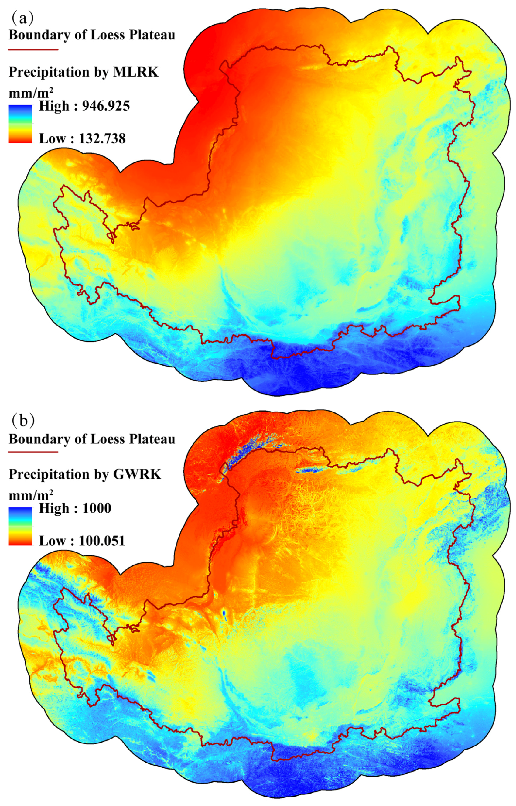
Based on background knowledge of the physical geography of the study area, the geographic factors that are closely related to local precipitation are selected as auxiliary variables. This process can help improve the accuracy of the RK model. 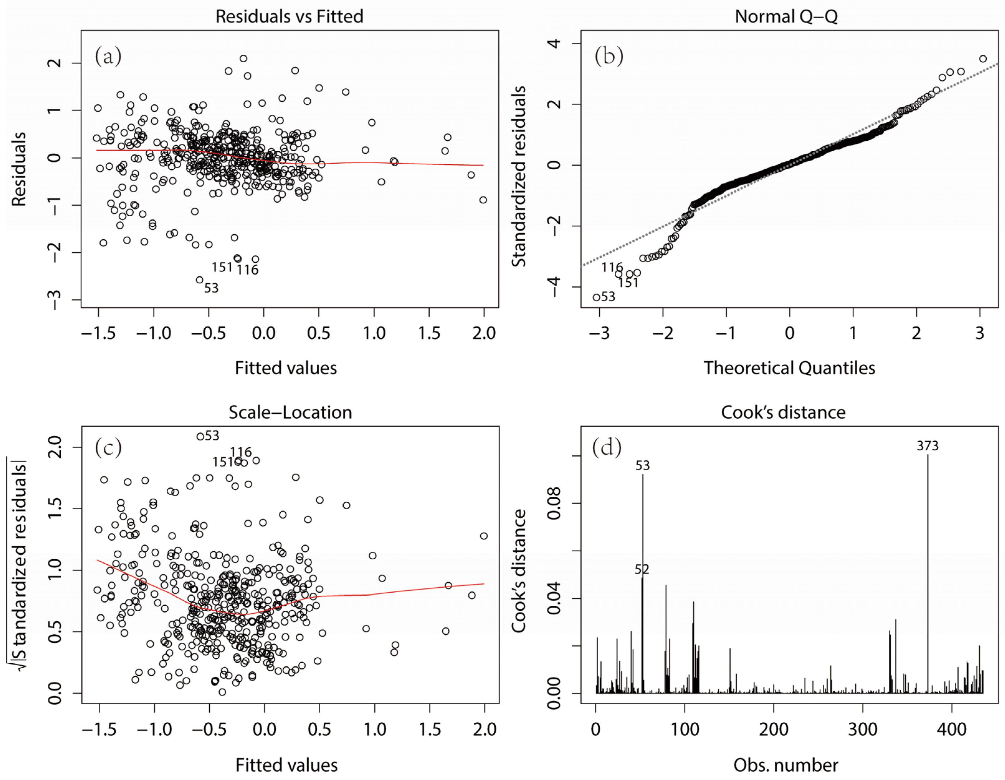The results of this study show that the average annual precipitation in the Loess Plateau gradually decreased from southeast to northwest under the influence of the monsoon and the sea (Figure 9). Affected by complex mountainous terrain, precipitation changed greatly in the Taihang Mountains and Luliang Mountain region in the east of the Loess Plateau. Precipitation in the narrow region windward and to the east of the Taihang Mountains was significantly higher than in the leeward area of the western mountains and the plain area on the east side of the mountains. Due to the Tibetan Plateau, the elevation of the western region of the Loess Plateau gradually increases, and the rainfall increases correspondingly. The Loess Plateau belongs to semi-humid and semi-arid areas, where water availability is an important limiting factor for vegetation growth. Vegetation typically thrives in places where rainfall is abundant. Moreover, if the precipitation changes significantly, the underlying natural geographical factors would also show a marked change. For example, in this study, the reason that station 373 had such a strong influence on observations is that it lies on the Huashan Mountain, where altitude is much higher than the surrounding areas.

By exploring the characteristics of the annual average rainfall data, a suitable interpolation method can be chosen for precipitation predictions. Geostatistical interpolation and non-geostatistical interpolation methods both involve various assumptions. In order to obtain a more accurate prediction, the data need to meet the assumed requirement [22,32]. For example, in order to make the distribution of data meet the requirements of the normality assumption, precipitation data were typically adjusted to a logarithmic scale. Of course, it is also possible to use an interpolation method that does not require a normality requirement calculation.

In choosing a suitable interpolation method, it is import to consider whether there is a need for precipitation data to fit trends in the interpolation process, and then further consider whether to fit the global trend or local trends according to the stability of the underlying surface. In this study, MLRK is a global trend-fitting method, which is suitable for a relatively homogeneous underlying surface, and GWRK is a local area trend-fitting method, which is suitable for relatively complex surface types [23,33]. Previous studies suggest that accuracy of the local trend-fitting method is generally higher than the overall trend-fitting method [5,19,26]; however, this is not always true. With an increase in the size of the study area and the complexity of the underlying surface, the relationship between rainfall and auxiliary variables will become more unstable. When the underlying surface changes greatly but precipitation is relatively stable, the variability in predicted rainfall may be overestimated in local trend fitting, thus reducing the accuracy of forecasts. This type of situation was recognized in this study. The results showed that the entire GWRK error was slightly larger than the MLRK error. In summary, it is difficult to choose the right interpolation method when starting a precipitation interpolation. The advisable way to obtain better interpolation results is by selecting several available interpolation methods, comparing the error after interpolation, and then selecting the method with the minimum error.

The interpolation result of annual average rainfall is affected by several uncertainty factors: (1) an uneven distribution and limited number of stations leads to the underestimation of trends and rainfall variability in these areas; (2) since the relationship between rainfall data and the auxiliary variable is unstable, a more accurate model cannot be precisely established, decreasing the interpolation result accuracy; (3) rainfall station data in most studies are limited to within the study area. A significant prediction error in interpolation appears at the boundary of the study area, known as “edge effects.” These effects could be mitigated by taking into account the precipitation data of stations just outside the border [15]. In this study, the precipitation data of meteorological stations located at the 100 km peripheral buffer of Loess Plateau was added in order to improve the prediction results of the study area boundary.

Measuring the interpolation error is an important process in interpolation method selection and analysis of interpolation results. In this study, two common methods were used to evaluate the results of interpolation: one using the predictive data set itself with cross-validation; the other using a verification data set to directly calculate ME, RMSE, and other indexes. When using the validation data set, the validation points should cover a broad range of land use types. In this study, the meteorological data of the validation data set is only from hydrological stations at the edge of a river or gully with lush vegetation coverage. This validation data set is therefore lacking in data from other land use types. Therefore, this study can clearly show that MLRK prediction performance was slightly better than GWRK in the area around the river, but in regions with other types of land use, it is not possible to determine which of the two models is better.

6. Conclusions

One of the main objectives of this study was to generate a highly accurate distribution map of average annual precipitation with a 500 m spatial resolution in the Loess Plateau for the period of 1980–2010. Alternative distribution maps of precipitation were interpolated by MLRK and GWRK methods and all showed a high accuracy. There were large disparities, however, in two regression Kriging processes using different methods: the variance explanation of the GWRK regression model was higher than that of MLRK, but the contrary is true of the Kriging process. The interpolation maps using MLRK and GWRK both captured many details of spatial distribution influenced by predictors. Although the GWRK is based on the spatial non-stationary assumption and the map predicted by GWRK did show greater spatial variation, the final validation analysis revealed that MLRK yielded higher model efficiency than GWRK, with small differences. This is in contrast to other previous precipitation interpolation studies. The conclusions can be summarized as follows: (1) both MLRK and GWRK are able to incorporate multiple auxiliary environmental factors into the modelling process and obtain a highly accurate precipitation distribution map; (2) unlike other studies of precipitation prediction, MLRK is shown to be a better method for precipitation interpolation when the underlying surface is complex. In future, greater effort should be made to consider more physical geographic factors related to or impacted by rainfall as auxiliary environmental variables, which could possess a higher resolution, in order to get a higher accuracy of precipitation distribution maps. More studies should investigate and identify the standards and principles to select and validate the interpolation methods further.

References

1. Taesombat, W.; Sriwongsitanon, N. Areal rainfall estimation using spatial interpolation techniques. Sci. Asia 2009, 35, 268–275. [Google Scholar] [CrossRef]
2. Li, X.; Gao, S. Precipitation Modeling and Quantitative Analysis; Springer Science & Business Media: Dordrecht, The Netherlands, 2012. [Google Scholar]
3. Shi, T.; Yang, X.; Christakos, G.; Wang, J.; Liu, L. Spatiotemporal interpolation of rainfall by combining BME theory and satellite rainfall estimates. Atmosphere 2015, 6, 1307–1326. [Google Scholar] [CrossRef]
4. Mair, A.; Fares, A. Comparison of rainfall interpolation methods in a mountainous region of a tropical island. J. Hydrol. Eng. 2010, 16, 371–383. [Google Scholar] [CrossRef]
5. Sun, W.; Zhu, Y.; Huang, S.; Guo, C. Mapping the mean annual precipitation of China using local interpolation techniques. Theor. Appl. Climatol. 2015, 119, 171–180. [Google Scholar] [CrossRef]
6. Xu, W.; Zou, Y.; Zhang, G.; Linderman, M. A comparison among spatial interpolation techniques for daily rainfall data in Sichuan Province, China. Int. J. Climatol. 2015, 35, 2898–2907. [Google Scholar] [CrossRef]
7. Jin, Q.; Shi, M.; Zhang, J.; Wang, S.; Hu, Y. Calibration of rainfall erosivity calculation based on TRMM data: A case study of the upriver basin of Jiyun River, North China. Sci. Soil Water Conserv. 2015, 13, 94–102. (In Chinese) [Google Scholar]
8. Seo, Y.; Kim, S.; Singh, V.P. Estimating spatial precipitation using regression kriging and artificial neural network residual kriging (RKNNRK) hybrid approach. Water Resour. Manag. 2015, 29, 2189–2204. [Google Scholar] [CrossRef]
9. Wong, D.W.; Yuan, L.; Perlin, S.A. Comparison of spatial interpolation methods for the estimation of air quality data. J. Expo. Sci. Environ. Epid. 2004, 14, 404–415. [Google Scholar] [CrossRef] [PubMed]
10. Li, H.; Hong, Y.; Xie, P.; Gao, J.; Niu, Z.; Kirstetter, P.; Yong, B. Variational merged of hourly gauge-satellite precipitation in Chia: Preliminary results. J. Geophys. Res. Atmos. 2015, 120, 9897–9915. [Google Scholar] [CrossRef]
11. Sideris, I.V.; Gabella, M.; Erdin, R.; German, U. Real-time radar-rain-gauge merging using spatio-temporal co-kriging with external drift in the alpine terrain of Switzerland. Q. J. R. Meteor. Soc. 2014, 140, 1097–1111. [Google Scholar] [CrossRef]
12. Newman, A.J.; Clark, M.P.; Craig, J.; Nijssen, B.; Wood, A.; Gutmann, E.; Mizukami, N.; Brekke, L.; Arnold, J.R.; Arnold, J.R. Gridded ensemble precipitation and temperature estimates for the contiguous United States. J. Hydrometeorol. 2015, 16, 2481–2500. [Google Scholar] [CrossRef]
13. Xie, P.; Xiong, A.Y. A conceptual model for constructing high-resolution gauge-satellite merged precipitation analyses. J. Geophys. Res. Atmos. 2011, 116, D21106. [Google Scholar] [CrossRef]
14. Michaelides, S.C. (Ed.) Precipitation: Advances in Measurement, Estimation and Prediction; Springer Science & Business Media: Berlin, Germany, 2007; pp. 131–169.
15. Bajat, B.; Pejović, M.; Luković, J.; Manojlović, P.; Ducić, V.; Mustafić, S. Mapping average annual precipitation in Serbia (1961–1990) by using regression kriging. Theor. Appl. Climatol. 2013, 112, 1–13. [Google Scholar] [CrossRef]
16. Masson, D.; Frei, C. Spatial analysis of precipitation in a high-mountain region: Exploring methods with multi-scale topographic predictors and circulation types. Hydrol. Earth Syst. Sci. 2014, 18, 4543–4563. [Google Scholar] [CrossRef]
17. Hutchinson, M.F. Interpolating mean rainfall using thin plate smoothing splines. Int. J. Geog. Inf. Syst. 1995, 9, 385–403. [Google Scholar] [CrossRef]
18. Ninyerola, M.; Pons, X.; Roure, J.M. A methodological approach of climatological modelling of air temperature and precipitation through GIS techniques. Int. J. Clim. 2000, 20, 1823–1841. [Google Scholar] [CrossRef]
19. Bostan, P.A.; Heuvelink, G.B.M.; Akyurek, S.Z. Comparison of regression and kriging techniques for mapping the average annual precipitation of Turkey. Int. J. Appl. Earth Obs. 2012, 19, 115–126. [Google Scholar] [CrossRef]
20. Li, J.; Heap, A.D. Spatial interpolation methods applied in the environmental sciences: A review. Environ. Model. Softw. 2014, 53, 173–189. [Google Scholar] [CrossRef]
21. Odeha, I.O.A.; McBratney, A.B.; Chittleborough, D.J. Spatial prediction of soil properties from landform attributes derived from a digital elevation model. Geoderma 1994, 63, 197–214. [Google Scholar] [CrossRef]
22. Hengl, T.; Heuvelink, G.B.; Stein, A. A generic framework for spatial prediction of soil variables based on regression-kriging. Geoderma 2004, 120, 75–93. [Google Scholar] [CrossRef]
23. Song, X.; Brus, D.; Liu, F.; Li, D.; Zhao, Y.; Yang, J.; Zhang, G. Mapping soil organic carbon content by geographically weighted regression: A case study in the Heihe River Basin, China. Geoderma 2016, 261, 11–22. [Google Scholar] [CrossRef]
24. Kumar, S.; Lal, R.; Liu, D. A geographically weighted regression kriging approach for mapping soil organic carbon stock. Geoderma 2012, 189, 627–634. [Google Scholar] [CrossRef]
25. Wang, Q.X.; Fan, X.H.; Qin, Z.D.; Wang, M.B. Change trends of temperature and precipitation in the Loess Plateau Region of China, 1961–2010. Global Planet. Chang. 2012, 92, 138–147. [Google Scholar] [CrossRef]
26. Harris, P.; Fotheringham, A.S.; Crespo, R.; Charlton, M. The use of geographically weighted regression for spatial prediction: An evaluation of models using simulated data sets. Math Geosci. 2010, 42, 657–680. [Google Scholar] [CrossRef]
27. Li, Z.; Zheng, F.L.; Liu, W.Z.; Flanagan, D.C. Spatial distribution and temporal trends of extreme temperature and precipitation events on the Loess Plateau of China during 1961–2007. Quat. Int. 2010, 226, 92–100. [Google Scholar] [CrossRef]
28. Wei, J.; Zhou, J.; Tian, J.; He, X.; Tang, K. Decoupling soil erosion and human activities on the Chinese Loess Plateau in the 20th century. Catena 2006, 68, 10–15. [Google Scholar] [CrossRef]
29. Wang, K.; Zhang, C.; Li, W. Comparison of geographically weighted regression and regression kriging for estimating the spatial distribution of soil organic matter. GISci. Remote Sens. 2012, 49, 915–932. [Google Scholar] [CrossRef]
30. Xin, Z.; Yu, X.; Li, Q.; Lu, X.X. Spatiotemporal variation in rainfall erosivity on the Chinese Loess Plateau during the period 1956–2008. Reg. Environ. Chang. 2011, 11, 149–159. [Google Scholar] [CrossRef]
31. Pebesma, E.J. Multivariable geostatistics in S: The gstat package. Comput. Geosci. 2004, 30, 683–691. [Google Scholar] [CrossRef]
32. Hengl, T. A Practical Guide to Geostatistical Mapping, 2nd ed.; University of Amsterdam: Amsterdam, The Netherlands, 2009. [Google Scholar]
33. Fotheringham, A.S.; Brunsdon, C.; Charlton, M. Geographically Weighted Regression: The Analysis of Spatially Varying Relationships; John Wiley & Sons Ltd.: Chichester, UK, 2002. [Google Scholar]
34. Cleveland, W.S. Robust locally weighted regression and smoothing scatterplots. J. Am. Stat. Assoc. 1979, 74, 829–836. [Google Scholar] [CrossRef]
35. Lado, L.R.; Polya, D.; Winkel, L.; Berg, M.; Hegan, A. Modelling arsenic hazard in Cambodia: A geostatistical approach using ancillary data. Appl. Geochem. 2008, 23, 3010–3018. [Google Scholar] [CrossRef]
Figure 1. Underlying surface features of the Loess Plateau (a); and location of meteorological and hydrologic stations (b).
Water 08 00266 g001
Figure 2. Structural characteristics of annual average precipitation at meteorological stations. (a) Distribution of annual average precipitation; and (b) correlation of precipitation for different stations at certain lag distance ranges.
Water 08 00266 g002
Figure 3. Mapped Z scores of Gi statistics for meteorological stations.
Water 08 00266 g003
Figure 4. Relationship between logit-transformed precipitation (PreT) and main environmental variables, including the standardized normal variable of NDVI (a); the standardized normal variable of DEM (b); the standardized normal variable of Slope (c); and the standardized normal variable of solar radiation (d).
Water 08 00266 g004
Figure 5. Diagnostic plots for multiple linear regression analysis. (a) is the scatter plot for the regression-predicted values versus the corresponding residuals; (b) is the normal Q-Q diagram; (c) is the scale-location graph; and (d) is the Cook’s distance diagram.
Water 08 00266 g005
Figure 6. Maps of GWR coefficients and local adjusted R2. (a) is the distribution of DEM coefficient; (b) is the distribution of slope coefficient; (c) is the distribution of NDVI coefficient; (d) is the distribution of north aspect coefficient; (e) is the distribution of northwest aspect coefficient; and (f) is the distribution of local R2.
Water 08 00266 g006
Figure 7. Comparison of regression coefficients between GWR and MLR. The orange points represent the mean of predicator coefficients in GWR, and the blue points represent the regression coefficients of MLR.
Water 08 00266 g007
Figure 8. Residual variograms and models fitted for (a) MLRK; and (b) GWRK.
Water 08 00266 g008
Figure 9. Precipitation climatology map of the 30 years (1980–2010) at Loess Plateau predicted by MLRK (a) and GWRK (b).
Water 08 00266 g009