Article

Spatiotemporal Distributions of Sr and Ba along an Estuarine River with a Large Salinity Gradient to the Gulf of Mexico

School of Renewable Natural Resources, Louisiana State University Agricultural Center, Baton Rouge, LA 70803, USA
*
Author to whom correspondence should be addressed.
Water 2016, 8(8), 323; https://doi.org/10.3390/w8080323
Submission received: 8 June 2016 / Revised: 26 July 2016 / Accepted: 27 July 2016 / Published: 1 August 2016

Abstract

:
Strontium and barium to calcium ratios are often used as proxies for tracking animal movement across salinity gradients. Many estuarine rivers face saltwater intrusion due to sea level rise, potentially causing changes in mobility and distribution of these metals upstream. From May 2013 to August 2015, monthly water samples were collected and in-situ measurements were performed at six sites along an estuary strongly affected by saltwater intrusion, the Calcasieu River, with salinity ranging from 0.02 to 29.50 Parts Per Thousand (ppt). Results showed that the total Sr concentration and the Sr/Ca ratio both increased significantly with increasing salinity. The average Sr concentration at the site closest to the Gulf of Mexico (Site 6) was 46.21 µmol/L, about 130 times higher than that of the site furthest upstream (Site 1, 0.35). The average Sr/Ca ratio at Site 6 (8.41 mmol/mol) was about three times the average Sr/Ca ratio at Site 1 (2.89). However, the spatial variation in total Ba concentration was marginal, varying from 0.36 to 0.47 µmol/L. The average Ba/Ca ratio at Site 1 (4.82 mmol/mol) was about 54 times the ratio at Site 6 (0.09), showing a negative relation between the Ba/Ca ratio and salinity. All elemental concentrations and ratios had considerable seasonal variations, with significant differences among sampling months for the Sr and Ba concentrations and the Ba/Ca ratio (p < 0.01). The results suggest that for low-gradient estuarine rivers such as the Calcasieu River, water chemistry upstream would experience substantial Sr and Ca enrichment, potentially affecting aquatic environments and biological communities.

Graphical Abstract

1. Introduction

Estuarine systems face a variety of threats ranging from regional anthropogenic factors, such as river basin land use change [1,2], riverine nutrient enrichment [3,4], and coastal industrial pollution [5], to global stressors such as climate change and sea level rise [6,7]. This is especially true for lowland estuarine rivers where any rise in sea level can have a far-reaching impact on the community. Over the past century, the global mean sea level has increased by nearly 200 mm [8,9] due to an increase in 20th century ocean heat content [10] and mass increase [11]. The rise rate was found to be accelerating in the past two decades, averaging 3.2 mm per year in a range between 2.8 and 3.6 mm [12].
As sea level rise continues, saltwater intrudes upstream inland, which can cause changes in water chemistry, especially salinity and pH. Salinity and pH are two important factors affecting many chemical and biological processes in estuarine waters. One of the processes is the adsorption–desorption of trace metals in estuarine mixing zones. Salinity and pH have been found to strongly affect mobility and flux rates of trace metals [13] when they are carried by rivers to various estuarine/coastal systems around the world; for instance, in the Galveston Bay estuary in Texas [14], the San Francisco Bay Estuary in California [15], the Changjiang Estuary in China [16,17], the Bang Pakong Estuary in Thailand [18], the Scheldt Estuary in the Netherlands [19], and the Conwy Estuary in North Wales [20]. The ongoing saltwater intrusion in the world’s estuaries may shift metal mobilization and precipitation landwards, the occurrence and effects of which are not well investigated. Such knowledge can be useful for future coastal resource management especially in low-lying, flat areas such as southern Louisiana where the estuaries extend 30 to 70 km inland.
The fate of trace metals in estuaries has been a great concern for aquatic life systems. Studies reported that high levels of strontium (Sr) and barium (Ba) concentrations could be toxic for marine embryos (abnormal shell calcification and embryo morphology) [21], benthic biota [22], and photosynthetic microorganisms [23]. For instance, Spangenbery and Cherr [21] showed that adverse effects on mussel embryos occurred when Ba concentration was between 200 and 900 μg/L. In addition to their natural occurrence, the level of trace metals in waterways could be elevated from petrochemical industry [24]. Offshore oil and gas drilling use two primary types of drilling fluids: water-based fluids and non-aqueous drilling fluids. Both of these fluids contain Ba as a major component [25,26]. Lira et al. [22] concluded that oil and gas drilling activities may potentially have important implications for meiobenthos through the toxicity of Ba. Southern Louisiana is a national center of the USA oil and petrochemical industry, and many processing plants are located along the estuaries. It is unknown if there is any elevated level of Ba in the estuarine waters in this region.
Determining movements and migrations of aquatic animals between environments is important, especially for the understanding of the life history characteristics of these animals. In complicated environments, such as estuaries, the movements and migrations of animals are affected by multiple factors [27]. Instead of using conventional tags, many animals have natural tags that can be used to answer ecological questions regarding their life histories. For instance, the elements present within otoliths (earbones) of fish are ideally suited to be used as natural tags, because elements, such as Sr and Ba, can be incorporated into their calcium carbonate matrix (CaCO3) through either substitution (e.g., BaCO3 or SrCO3) or binding within the lattice matrix [28,29]. Studies have shown that the ambient Sr/Ca and Ba/Ca ratios and environmental conditions, including salinity, influence the Sr/Ca and Ba/Ca ratios in fish otoliths and scales [30,31]. For instance, fish with otolith Ba/Ca ≤ 5 μmol/mol were classified as resident in salt water, and those with ≥6 μmol/mol as resident in fresh water [27]. Therefore, Sr/Ca and Ba/Ca ratios have been used as proxies across salinity gradients to detect aquatic animal (such as fish) movements.
Louisiana’s coast of the northern Gulf of Mexico experienced rapid land subsidence and land loss in the past century [32,33,34]. As a result, the Louisiana Gulf coast has had one of the highest relative sea-level rises in the United States [35,36]. Saltwater intrusion has been observed in many coastal rivers in the region, and the Calcasieu River is a prime example. This river flows through the Chenier Plain comprising an area of approximately 5000 km2 with a west-east coastline of about 200 km [37], stretching geographically from approximately 29.5° N to 33.2° N and from 91.3° W to 94.0° W. The Calcasieu River is 322 km long with a drainage area of 9780 km2 [38], discharging into the Calcasieu Lake before the northern Gulf of Mexico. During the past half century, this river was hydrologically altered. For instance, along the Calcasieu River, two dams were constructed in its upper reach, and prior to the 1960s, a deep draft channel in the Calcasieu River from the Gulf of Mexico to Lake Charles allowed saltwater from the Gulf to migrate further inland. Taltwater, which kills many types of vegetation, began to destroy some of the sensitive wetlands of the Calcasieu River Basin. To solve the saltwater intrusion problem, the Calcasieu River Saltwater Barrier was constructed in the 1960s to prevent saltwater from traveling north further upstream as well as to regulate freshwater outflow [39,40]. In addition to saltwater intrusion, the lower Calcasieu River is a heavy shipping channel for petrochemical industry concentrated on the river banks. These two problems make the river estuary an ideal location to study the Sr and Ba dynamics across salinity gradients, as the aforementioned hydrological alterations may have had considerable effects on water quality and riverine metal transport.
Studies have been conducted on trace metals for the Mississippi River [41,42], which has a high volume of freshwater discharge pushing into the far-shore open water. On the other hand, little is known about trace metal dynamics in Louisiana’s small estuarine rivers like the Calcasieu that has low freshwater discharge and is strongly affected by tides and saltwater intrusion. Due to its highest rate of relative sea-level rise among all regions in the United States, the study of saltwater impacts on metal dynamics in southern Louisiana can provide information that will have global implications. The ultimate goal of this study is to investigate the impacts of saltwater intrusion on trace metal distribution. Specifically, this study is to quantify spatial and temporal variations of Sr, Ca, Ba, Sr/Ca, and Ba/Ca in the Calcasieu River and to assess mixing dynamics across salinity gradients for these same constituents.

2. Materials and Methods
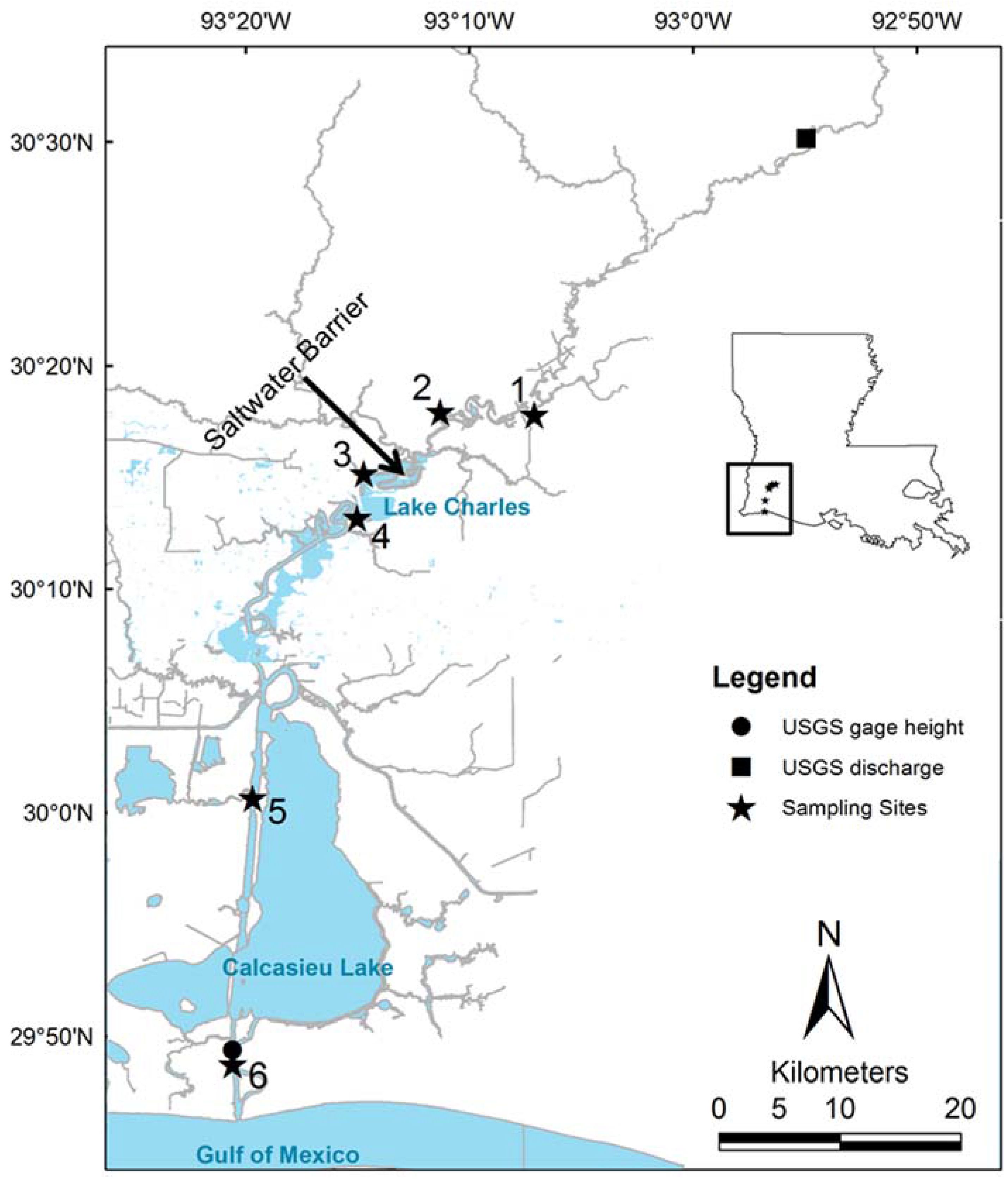
2.1. Study Area

The study area is the lower reach of the Calcasieu River that enters the northern Gulf of Mexico in southwest Louisiana, USA (Figure 1). Six sampling sites were selected along the 88-km reach and they are all within the Calcasieu Parish (north) and the Cameron Parish (south). In the study area, the main soil types (>65%) are: Arat mucky silt loam (AR), Bancker muck (BA), Creole mucky clay (CR), Clovelly muck (CO), Crowley-Vidrine (Cr), Guyton-Messer silt loams (Gy), Gentilly muck (GC), Kinder-Gist complex (Kd), Mowata-Vidrine complex (Mt), Edgerly loam (Mr), Scatlake mucky clay (SC), and Udifluvents (UA) [43].
The climate of the study area is characterized by long, hot, and humid summers and generally short, mild winters. Land use in the north part of the study area (Calcasieu Parish) is primarily agriculture. More than 65% of the land is used as cultivated cropland, pastureland, and woodland, and most of the remaining acreage is used as urban land, marshland, or swampland [44]. Most of the southern part of the study area (Cameron Parish) is coastal marshland. These marshes are used mainly as habitats for wildlife, rangeland, and oil and gas fields [45].

2.2. Data Collection

Long-term daily discharge (available since September 1922) and gage height (available since October 1997) data of the Calcasieu River was collected from the US Geological Survey (USGS). The gage stations were chosen based on their data availability and proximity to the sampling sites for optimal representation. Specifically, daily discharge was collected at the Calcasieu River near Kinder, LA (USGS 08015500), and the daily gage height was collected at the Calcasieu River near Cameron, LA (USGS 08017118) (Figure 1).

2.3. Water Sample Collection

From May 2013 to August 2015, monthly field trips (except June 2013, October 2013 and November 2014) were made to conduct in-situ measurements and collect water samples at six sampling sites along the Calcasieu River (Figure 1). Note that Site 3 was only sampled from August 2014 to August 2015. The saltwater barrier is located approximately two km downstream of Site 2, below which all sampling sites are affected by saltwater. During each trip, field measurements on water temperature, dissolved oxygen (DO) concentration, pH, and salinity were conducted using an YSI 556 multi-probe meter (YSI Inc., Yellow Springs, OH, USA). In addition, a 250 mL water sample was collected from each site for elemental analysis. The samples were acidified to pH < 2 at the time of collection in the field without filtration. A one-liter water sample was collected from each site for total suspended solids (TSS) analysis. High Density Polyethylene (HDPE) bottles were used to collect water samples, and all the bottles were thoroughly acid-cleaned before use. All the water samples were taken approximately 30–50 cm below the surface. The samples were collected from piers reaching out about 8–15 m into the river channel with a grab sampler consisting of a 12-ft aluminum pole with a polyethylene bottle attached at the end of the pole. On each trip, samples were collected in duplicate at one of the sites; however, subsequent analyses indicated typically less than 5% differences in all constituents. As a result, duplicates data were removed from the data analysis. All the water samples were stored in a cooler with wet ice during transportation, and refrigerated until analysis. All efforts were made to avoid any possible contamination in the field, during transportation, and in Laboratory. Table 1 shows the sampling sites’ information.

2.4. Water Sample Analysis

Water samples were analyzed for total recoverable concentrations of all elements and total suspended solids at the W. A. Callegari Environmental Center, Louisiana State University Agricultural Center using EPA Method 200.7. Briefly, water samples were digested using metals-grade concentrated HCl and HNO3. Yttrium was added to the water samples as an internal standard. Element concentrations above the calibration curve were diluted by factors of 10, 20, 50, 100, or 1000 to bring them into the calibration curve. Finally, the analyses were conducted using an Inductively Coupled Plasma Optical Emission Spectrometer (ICP-OES, Varian Vista MP-X, Palo Alto, CA, USA). The one-liter water samples collected from each site were filtered, whereby gravimetric analysis was used to determine TSS. Field and Laboratory blanks, and Independent/Continuing Calibration Verification/Blanks were used for quality control to insure that the samples were not contaminated, and that all sample analyses were within control limits. Laboratory duplicate measurements of a same water sample typically yielded a difference of less than 5%. The method detection limits in our study for Sr, Ca, Ba, and TSS are 0.0088 µmol/L, 0.50 µmol/L, 0.14 µmol/L, and 4 mg/L, respectively.

2.5. Statistical Analyses

Multivariate analysis of variance (MANOVA) was performed for all element concentration/ratio for main and interactive effects of sampling site and month on differences in concentrations/ratios. Two-way analyses of variance (ANOVAs) comparing water sample values were calculated separately for each of the five measured element concentrations and ratios according to sampling site and month of collection. Pearson correlations were compared between element concentrations and ratios and environmental parameters, including salinity, pH, temperature, dissolved oxygen (DO), and TSS, to investigate potential relationships. All statistical analyses were performed with the SAS Statistical Software package. All statistical tests and confidence intervals are reported at α = 0.01 critical level.

3. Results

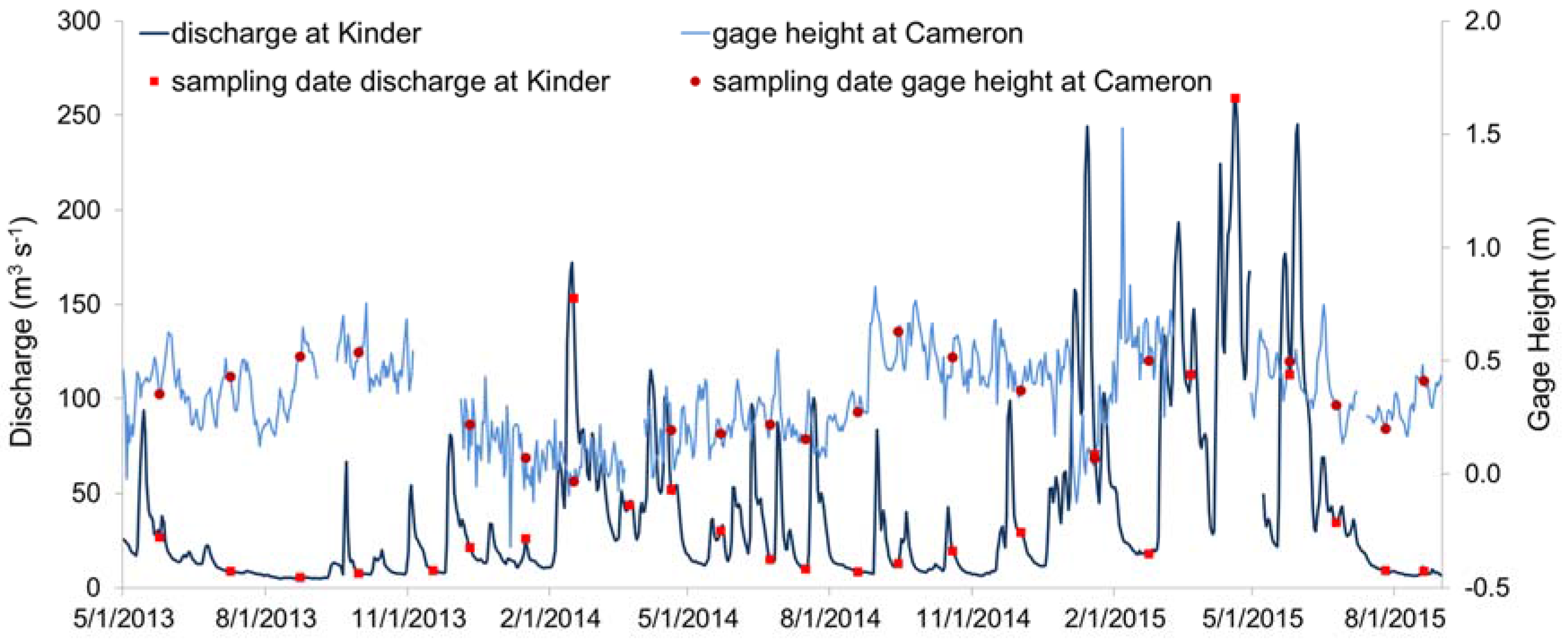
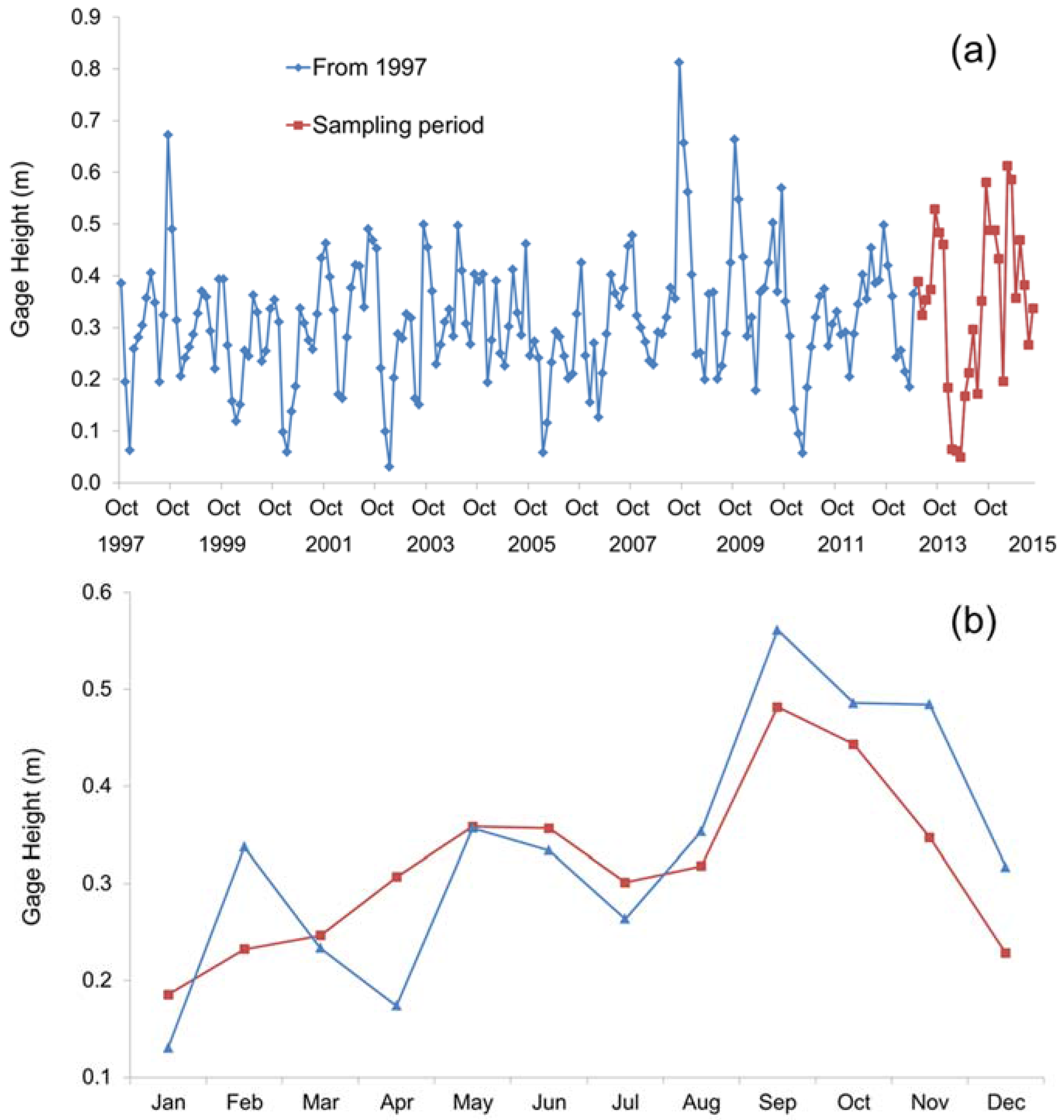
3.1. Hydrology and Ambient Conditions

From 1 May 2013 to 31 August 2015, the Calcasieu River showed an average daily discharge of 39 m3/s (standard deviation (std): ±46), ranging from 5 to 259 m3/s. The discharge during the sampling period was notably lower than the long-term average from 1980 to 2009 (72 ± 66 m3/s) [46]. Seasonally, the Calcasieu River showed higher discharge during the winter and spring months and lower discharge during the summer and fall months in the period from 1980 to 2009 [46]. During the sampling period, the river exhibited the same seasonal pattern as in the period from 1980 to 2009, with April having the highest average discharge (103 m3/s) and August the lowest (9 m3/s). During the 25 field sampling days from 1 May 2013 to 31 August 2015, the discharges ranged from 5 to 259 m3/s with an average of 44 m3/s (std: ±59) (Figure 2).
The Calcasieu River near its mouth at Cameron showed a long-term (October 1997–August 2015) average daily gage height (or tidal stage) of 0.31 m (±0.18), ranging from −0.48 to 2.31 m. Over the past eight years, the tidal stage showed a clear increasing trend (Figure 3a). During the two-year sampling period, the average daily gage height at Cameron ranged from −0.32 to 1.53 m, with an average of 0.34 m (±0.19). Seasonally, in contrast with the river discharge, the tidal stage at the river mouth was high in the fall months, with September having the highest monthly average (0.48 m), and low in the winter months, with January having the lowest (0.18 m). During the sampling period, the monthly average gage heights at the Calcasieu River near Cameron were similar to the historical monthly average gage heights, and the seasonal trend of gage height was similar to the historical trend, with larger variance (Figure 3b). During the 25 field trip days from May 2013 to August 2015, the average daily gage height at the Calcasieu River near Cameron ranged from −0.03 to 0.63 m, averaging 0.31 (std: ±0.18). The average daily gage heights at the Calcasieu River near Cameron were well represented by the average daily gage heights during the 25 field trip days (Figure 2).
The ambient conditions at the six sampling sites varied largely (Table 2). Salinities at Site 6 ranged from 4.80 to 29.50 ppt, with an average of 19.91, which is more than 280 times higher than the average salinity at Site 1. Salinity increased with the decrease of distance from the Gulf of Mexico. Overall, pH, DO concentration, and water temperature showed similar trends to salinity. During the 25 sampling trips, the average pH at all the sampling sites ranged from 6.08 at Site 2 to 8.18 at Site 6, while the average DO concentration ranged from 4.64 mg/L at Site 3 to 7.77 mg/L at Site 6. The average water temperature at Site 3 was higher than other sites, which is attributed to a different sampling schedule for Site 3. TSS concentrations varied from Site 1 to Site 6 and, overall, showed relatively low levels (mostly <20 mg·L−1) in the four upstream sites (Table 2, Figure 4e). All six sites had higher salinity during summer and fall months (Figure 4a). From March to November, pH exhibited an increasing trend (Figure 4b). As expected, June, July, and August had higher water temperatures, while December, January, and February had lower (Figure 4c). The dissolved oxygen (DO) concentration had the opposite trend from water temperature (Figure 4d). Correlation analysis showed that temperature and DO concentration were negatively highly correlated (Table 3). Sites 5 and 6 had higher TSS variation seasonally, but there was no clear trend (Figure 4e).

3.2. Strontium, Ca Concentrations and Sr/Ca Ratio

During the sampling period, the Sr concentration showed a considerable variation among sampling sites, with sites closer to the Gulf having much higher concentrations (Table 4). The average Sr concentration at Site 6 was 46.21 µmol/L, about 130 times higher than that at the stream Site 1 (0.35 µmol/L). The spatial difference in Sr concentration was statistically significant (both p < 0.01, Table 5 and Table 6). Seasonally, there was also a large variation in Sr concentration at each site: from not detected (n.d.) to 1.71 µmol/L at Site 1, from n.d. to 7.19 µmol/L at Site 2, from 0.23 to 18.26 µmol/L at Site 3, from 0.34 to 35.61 µmol/L at Site 5, from 1.60 to 63.00 µmol/L at Site 5, and from 10.61 to 74.18 µmol/L at Site 6. In general, all six sites had higher Sr concentrations during the summer and fall months (Figure 5a), and the difference in monthly Sr concentration was statistically significant (both p < 0.01, Table 5 and Table 6). In the interactive effect of sampling site and month, the Sr concentration showed no significant differences (both p > 0.01, Table 5 and Table 6).
The Ca concentration was significantly different among sampling sites (both p < 0.01, Table 5 and Table 6), with sites closer to the Gulf having much higher concentrations (Table 4). The average Ca concentration at Site 6 was 8.19 mmol/L, about 60 times higher than Site 1 (0.13 mmol/L). The Ca concentration varied largely at all the sampling sites: from 0.06 to 0.92 mmol/L at Site 1, from 0.07 to 2.64 mmol/L at Site 2, from 0.07 to 2.07 mmol/L at Site 3, from 0.08 to 5.51 mmol/L at Site 5, from 0.24 to 18.25 mmol/L at Site 5, and from 1.22 to 45.76 mmol/L at Site 6. Seasonally, the Ca concentration had a large variation, with August having the highest concentration of all six sites except Site 6 (Figure 5b). Furthermore, there was no statistically significant difference among sampling months (p > 0.01, Table 6). In the interactive effect of sampling site and month, the Ca concentration showed no significant differences (both p > 0.01, Table 5 and Table 6).
The Sr/Ca ratio increased with the decrease of distance to the Gulf and the spatial difference in the Sr/Ca ratio was statistically significant (both p < 0.01, Table 5 and Table 6). The average Sr/Ca ratio at Site 6 (8.41 mmol/mol) was about three times the average Sr/Ca ratio at Site 1 (2.89 mmol/mol). Seasonally, the Sr/Ca ratio varied largely at all sampling sites: from 0 to 4.14 mmol/mol at Site 1, from 0 to 6.48 mmol/mol at Site 2, from 2.46 to 8.82 mmol/mol at Site 3, from 4.32 to 20.83 mmol/mol at Site 5, from 2.92 to 34.16 mmol/mol at Site 5, and from 1.23 to 28.53 mmol/mol at Site 6. There was no clear seasonal trend of the Sr/Ca ratio at Sites 1 and 2, while the other four sites had large variations, with July having the highest Sr/Ca ratio for Sites 4, 5, and 6 (Figure 5c). There was no statistically significant difference among sampling months (p > 0.01, Table 6).

3.3. Barium Concentration and Ba/Ca Ratio

Overall, spatial variation in Ba concentration was small among the six sites, from 0.36 µmol/L at Site 6 to 0.47 µmol/L at Site 5. However, there was significant difference in Ba concentration among sampling sites (both p < 0.01, Table 5 and Table 6). Temporal variation of Ba concentration was larger (from one to three fold), but relatively smaller when compared with the spatial variation of Sr and Ca concentrations (Table 4 and Figure 5d). There was significant difference of Ba concentration among sampling months (both p < 0.01, Table 5 and Table 6), with winter months having lower Ba concentrations (Figure 5d). There was no statistically significant difference in the interactive effect of sampling site and month (both p > 0.01, Table 5 and Table 6).
Unlike the Sr/Ca ratio, the Ba/Ca ratio decreased with decreasing distance to the Gulf of Mexico, and the spatial difference in the Ba/Ca ratio was statistically significant (both p < 0.01, Table 5 and Table 6). The average Ba/Ca ratio at Site 1 (4.82 mmol/mol) was about 54 times the average ratio at Site 6 (0.09 mmol/mol). Temporally, the Ba/Ca ratio varied largely at all sampling sites: from 0.55 to 9.21 mmol/mol at Site 1, from 0.16 to 7.24 mmol/mol at Site 2, from 0.11 to 5.96 mmol/mol at Site 3, from 0.09 to 5.68 mmol/mol at Site 5, from 0.02 to 2.15 mmol/mol at Site 5, and from 0.01 to 0.36 mmol/mol at Site 6. Seasonally, the Ba/Ca ratio had large variation and there was significant difference among sampling months (both p < 0.01, Table 5 and Table 6). In general, all six sites had higher Ba/Ca ratios during spring and fall months (Figure 5e). The Ba/Ca ratio was no significantly different in the interactive effect of sampling site and month (both p > 0.01, Table 5 and Table 6).

3.4. Relationships between Concentrations and Ratios of Sr, Ba, and Ca and Environmental Parameters

The Sr and Ca concentrations were positively correlated to salinity, pH, DO, and TSS, while no clear correlation of these concentrations with water temperature was found (Table 3). The Sr/Ca ratio was positively correlated to salinity and pH, but not correlated to temperature, DO, and TSS (Table 3). In contrast with other element concentrations and ratios, the Ba concentration was positively correlated to temperature and negatively correlated to DO, while no correlation was found between Ba concentration and salinity, pH, and TSS (Table 3). The Ba/Ca ratio was negatively correlated to salinity and pH, but not correlated to temperature, DO, and TSS (Table 3).

4. Discussion

Dissolved Sr loads in the world’s river waters have been reported by Gaillardet et al. to have the largest variation when compared with other trace metals [47]. These loads ranged from a few ng/L to nearly 100 µg/L, with an average of 60 µg/L. On the other hand, dissolved Ba loads in the world’s river waters are among the least variable, ranging between 10 and nearly 100 µg/L with an average of 23 µg/L [47]. Similar to Sr, dissolved Ca concentrations in freshwaters can be highly variable, potentially reaching very low levels, e.g., <1–20 mg/L [48,49]. In this study, a very similar trend was found: Sr and Ca loads in river water samples collected above the saltwater barrier (freshwater) varied largely (0.35–0.77 µmol/L or 31–67 µg/L for Sr, and 0.13–0.23 mmol/L or 5.21–9.22 mg/L for Ca), both spatially and temporally, while Ba loads showed little change (0.42–0.46 µmol/L or 58–63 µg/L) in the same samples. The variations of element concentrations will in turn result in variations of element ratios. Variations of element concentrations and ratios include spatial and temporal variations. Spatial and temporal variations are discussed separately below.

4.1. Spatial Variation

The Sr and Ca concentrations in marine waters are significantly higher than in freshwaters due to different geological compositions of marine and fresh water systems [50,51]. Brown and Severin reported average marine water Sr and Ca concentrations of 7.64 ± 0.53 mg/kg (87.19 ± 6.05 µmol/L) and 405.87 ± 27.49 mg/kg (10.13 ± 0.68 mmol/L), respectively [50]. The Sr and Ca concentrations in the Calcasieu River were lower than the average marine water Sr and Ca concentrations (Table 4). However, the Sr/Ca ratio in our study was fairly close to the average marine Sr/Ca ratio (8.61 mmol/mol, range: 8.17 to 8.87), and was much higher than the median river water Sr/Ca ratio (2.39 mmol/mol, range: 0.27 to 19.18) [50] (Table 4). According to Brown and Severin [50], the Sr/Ca ratio varied across a wider range in river environments than in marine environments, with less than 3% of the 786 rivers reviewed having median Sr/Ca levels that exceeded minimum marine levels. In the Calcasieu River, two (Sites 5 and 6) out of six sampling sites had Sr/Ca ratios that exceeded the minimum marine levels.
The Ba concentrations found in the Calcasieu River were higher than those found in the majority of surface and municipal water supplies in the USA (≤0.03 mg/L or ≤0.22 µmol/L) [52]. New and expanded industrial Ba uses are studied in Kravchenko et al. 2014 [53]. For instance, BaSO4 is commonly used as a contrast agent in medical imaging studies (X-ray). Because of its high molecular weight, approximately 94% of barite mined today is used as a wetting agent or component of drilling mud for oil and gas drilling [54]. In this study, however, there is no evidence suggesting any effect from the surrounding petrochemical industry on the concentration level of Ba. Sites 1 and 2, which are located above the saltwater barrier and petrochemical plants, showed a similar or even slightly higher level of Ba concentration than the other sites that are close to the chemical plants and the Gulf (Table 4). Previous studies found that dissolved Ba in natural waters is largely determined by the geological composition of the streambed and weathering processes [47]. For instance, Ba is often rich in the geographic areas characterized by volcanic terrains, specifically alkaline-rich volcanic products or detrital (sedimentary) volcanic by-products (e.g., black shales) [55,56]. The levels of Ba concentration found in this study may indicate the role of geological origin of Ba.
Ba is usually elevated in fresh waters and then exhibits an oligohaline maximum, and shows generally conservative mixing afterwards for the remainder of the salinity range [51,57]. However, the mixing curves of Ba can be different from this pattern; for example, sampling season could play an important role in Ba distribution [58,59]. For the Calcasieu River, opening and closing of the Saltwater Barrier can affect the quantity of freshwater flow, which may alter the mixing dynamics of Ba in this system. The level of Ba concentration in this study was not related with salinity or pH. However, because of a close positive relation of Ca concentration with salinity, there was a strong negative relation between Ba/Ca ratio and salinity (Table 3). In their study on trace metals in coastal waters along the Texas coast, Walther and Nims [51] reported a wide range of the Ba/Ca ratio, 62 to 973 μmol/mol, similar to the Ba/Ca ratios found in our study at the two sites closest to the Gulf of Mexico (Sites 5 and 6). The fact that higher Ba/Ca ratios were found at other sites upstream suggests that freshwater discharge plays an important role in this elemental ratio. This finding may further suggest that large river systems with high freshwater flows will not be chemically affected by sea level rise as much as small coastal rivers with low freshwater flow will.
Strontium has been the most widely used trace metal to study aquatic animal movements between freshwater and marine habitats [60], and most studies of fish migration with otolith chemistry have used the Sr/Ca ratio. Recent studies have found that the Ba/Ca ratio may also be a sensitive indicator of freshwater residency [27,61,62]. However, not all constituents are equally effective as proxies. For instance, Walther and Nims [51] concluded that, in Texas systems, the capacity to detect animal movements across salinity gradients using the Sr/Ca ratio as a proxy will be more difficult compared to other systems, while using the Ba/Ca ratio as a proxy would be highly useful for tracking animal movements. In the Calcasieu River, the large spatial variations of the Sr/Ca and Ba/Ca ratios and the clear relationships between these ratios and salinity indicate that both would be very useful as proxies for tracking animal movement.

4.2. Temporal Variation

Understanding the causes of seasonal element concentrations and ratios in a coastal river can be complicated by interrelationships among potential control factors [63]. Shiller [63] showed that changes in suspended particulate matter, pH, and discharge appear unable to account for the observed element seasonal variability, but redox processes remained as the likely candidate for causing the most significant element seasonal variability [63]. In our study, as mentioned above, pH had an increasing trend from March to November. However, no element concentration or ratio showed the same trend. Therefore, pH itself was unable to explain the seasonal variability of element concentrations and ratios even though pH was significantly correlated to all the studied element concentrations and ratios except the Ba concentration.
Linear or nearly linear mixing of Sr and Ca across salinity gradients has been reported in estuaries worldwide [41,51,64,65,66]. In our study, mixing curves of both the Ca and Sr concentrations across the salinity gradient in the Calcasieu River were linear (Figure 6). The Sr concentration was highly correlated to salinity, which may have also been the driving factor for the seasonal variability of the Sr concentration. The seasonal trend of salinity was basically the same as the seasonal trend of the Sr concentration (Figure 4a and Figure 5a). Salinity may not be the driving factor for the seasonal variability of the Ca concentration, as well as the variability of the Sr/Ca and Ba/Ca ratios because of differences in seasonal trends (Figure 4a and Figure 5b–e ). Therefore, for the Ca concentration and the Sr/Ca, Ba/Ca ratios, salinity was the essential reason for seasonal variability in the elemental concentrations, in the interactions with other environmental factors including pH, DO and TSS.
In natural aquatic systems, the concentration of Ba depends on the mineral matrix of aquifer lithologies (e.g., sulfates, carbonates, granodiorite, and shale) as well as the physicochemical conditions (e.g., pH, temperature, and redox state) of the groundwater [53]. In general, Ba solubility increases with decreasing pH [67]. However, this was not the case in our study. The lack of or weak relationship between Ba concentration and environmental factors strongly indicate the role of geological origin of Ba.
Based on an examination of variability in mean trace element concentrations in the Mississippi River, Shiller [63] suggested that hydrologic factors may be important in determining trace element variability. This is, however, not the case in our data analysis. The reason for the lack of a relationship between discharge variability and element concentration and ratio variability might be due to the fact that the discharge records for the Calcasieu River come from a gauge station that is much further upstream than all the sampling sites. Future studies with nearby discharge measurements can be used to test the impact of discharge on variations of element concentrations and ratios, and also to calculate freshwater loadings of Sr and Ba to the Gulf of Mexico.
Due to the mixing of freshwater and saltwater, estuaries are extremely dynamic and complex environments. Sea level rise, which causes saltwater intrusion, will change the mixing point of freshwater and saltwater, which in turn, may have significant impact on biology. Due to its historic saltwater intrusion problem and the existence of the Calcasieu Saltwater Barrier, studies of metal dynamics in the Calcasieu River could have relevant implications for other similar systems worldwide. Current estimates of riverine metal fluxes are based entirely on measurements of dissolved metal concentrations, and neglect the impact of riverine particulate dissolution in seawater [68]. However, the riverine particulate dissolution in seawater could have considerable influence on the overall metal chemistry. For instance, the weathering of riverine particulate material upon arrival in coastal areas makes a significant contribution to the overall Sr chemistry of seawater over geological timescales [68,69]. Further studies of dissolved and particulate interaction are needed to better understand metal dynamics in the Calcasieu River.

5. Conclusions

This study investigated strontium, barium, and calcium concentrations and their ratios in an 88-km long estuarine reach with a salinity range from 0.02 to 29.50 ppt over two years. It is the first assessment on the spatial and temporal variations of these metals in an estuary for such a large salinity range and long period of time. The study found considerable spatiotemporal variation in the element concentrations and their ratios. Salinity strongly affects spatiotemporal distributions of Sr and Ca concentrations and their elemental ratios. Results showed that the total Sr concentration and the Sr/Ca ratio both increased significantly with increasing salinity. Total suspended solids concentration also plays a role in the element distribution. In contrast, salinity has no effect on Ba concentration, which appears mainly geochemically controlled. All elemental concentrations and ratios had considerable seasonal variations, with significant differences among sampling months for the Sr, Ba concentrations and the Ba/Ca ratio (p < 0.01). These results indicate that concentrations of Sr and Ca in the world’s estuaries will very likely increase in the future as sea level rise continues, and that the extent of these increases will depend on the extent of saltwater intrusion. For low-gradient estuarine rivers with low freshwater discharge, such as the Calcasieu River in southwest Louisiana, USA, water chemistry upstream would experience substantial Sr and Ca enrichment, which could affect aquatic environments and biological communities.

Acknowledgments

This study was financially supported through grants from the National Fish and Wildlife Foundation (Project No. 8004.12.036402) and the United States Department of Agriculture Hatch Funds (Project No. LAB94230). Thanks go to the US Geological Survey for making the long-term river discharge and gage height data available for this study and to Jeff Corkern for laboratory metal analysis at the Louisiana State University W.A. Callegari Environmental Center. The authors are grateful to many students including, among others, Paula Castello Blindt, Kaci Fisher, Sanjeev Joshi, and Zhen Xu for their outstanding field assistance.

Author Contributions

Songjie He carried out the study and analyzed the data, and wrote the first manuscript draft. Y. Jun Xu developed the study concept, provided oversight throughout the study, and revised the manuscript. All authors read and approved the final manuscript.

Conflicts of Interest

The authors declare no conflict of interest.

References

  1. Birch, G.F.; Lean, J.; Gunns, T. Growth and decline of shoreline industry in Sydney estuary (Australia) and influence on adjacent estuarine sediments. Environ. Monit. Assess. 2015, 187, 1–17. [Google Scholar] [CrossRef] [PubMed]
  2. Dorado, S.; Booe, T.; Steichen, J.; McInnes, A.S.; Windham, R.; Shepard, A.; Lucchese, A.E.B.; Preischel, H.; Pinckney, J.L.; Davis, S.E.; et al. Towards an understanding of the interactions between freshwater inflows and phytoplankton communities in a subtropical estuary in the Gulf of Mexico. PLoS ONE 2015, 10, e0130931. [Google Scholar] [CrossRef] [PubMed]
  3. Scavia, D.; Rabalais, N.N.; Turner, R.E.; Justic, D.; Wiseman, W.J. Predicting the response of Gulf of Mexico hypoxia to variations in Mississippi River nitrogen load. Limnol. Oceanogr. 2003, 48, 951–956. [Google Scholar] [CrossRef]
  4. Ferreira, V.; Castagneyrol, B.; Koricheva, J.; Gulis, V.; Chauvet, E.; Graca, M.A.S. A meta-analysis of the effects of nutrient enrichment on litter decomposition in streams. Biol. Rev. 2015, 90, 669–688. [Google Scholar] [CrossRef] [PubMed]
  5. Pinto, A.B.; Pagnocca, F.C.; Pinheiro, M.A.A.; Fontes, R.F.C.; de Oliveira, A.J.F.C. Heavy metals and TPH effects on microbial abundance and diversity in two estuarine areas of the southern-central coast of São Paulo State, Brazil. Mar. Pollut. Bull. 2015, 96, 410–417. [Google Scholar] [CrossRef] [PubMed]
  6. Geselbracht, L.L.; Freeman, K.; Birch, A.P.; Brenner, J.; Gordon, D.R. Modeled sea level rise impacts on coastal ecosystems at six major estuaries on Florida’s gulf coast: Implications for adaptation planning. PLoS ONE 2015, 10, e0132079. [Google Scholar] [CrossRef] [PubMed]
  7. Wang, G.D.; Kang, J.C.; Yan, G.D.; Han, G.Q.; Han, Q.C. Spatio-Temporal Variability of Sea Level in the East China Sea. J. Coast. Res. 2015, 73, 40–47. [Google Scholar] [CrossRef]
  8. Intergovernmental Panel on Climate Change (IPCC). Climate Change 2007: The Physical Science Basis. Available online: https://www.ipcc.ch/pdf/assessment-report/ar4/wg1/ar4_wg1_full_report.pdf (accessed on 7 June 2016).
  9. Church, J.A.; White, N.J. Sea level rise from the late 19th to the early 21st century. Surv. Geophys. 2011, 32, 585–602. [Google Scholar] [CrossRef]
  10. Munk, W. Twentieth century sea level: An enigma. Proc. Natl. Acad. Sci. USA 2002, 99, 6550–6555. [Google Scholar] [CrossRef] [PubMed]
  11. Miller, L.; Douglas, B.C. Mass and volume contributions to twentieth-century global sea level rise. Nature 2004, 428, 406–409. [Google Scholar] [CrossRef] [PubMed]
  12. Intergovernmental Panel on Climate Change (IPCC). Climate Change 2013: The Physical Science Basis. Available online: https://www.ipcc.ch/pdf/assessment-report/ar5/wg1/WGIAR5_SPM_brochure_en.pdf (accessed on 7 June 2016).
  13. Turner, A. Trace-metal partitioning in estuaries: Importance of salinity and particle concentration. Mar. Chem. 1996, 54, 27–39. [Google Scholar] [CrossRef]
  14. Wen, L.S.; Santschi, P.; Gill, G.; Paternostro, C. Estuarine trace metal distributions in Galveston Bay: Importance of colloidal forms in the speciation of the dissolved phase. Mar. Chem. 1999, 63, 185–212. [Google Scholar] [CrossRef]
  15. Sanudo-Wilhelmy, S.A.; Riviera-Duarte, I.; Flegal, A.R. Distribution of colloidal trace metals in the San Francisco Bay Estuary. Geochim. Cosmochim. Acta 1996, 60, 4933–4944. [Google Scholar] [CrossRef]
  16. Edmond, J.M.; Spivack, A.; Grant, B.C.; Hu, M.H.; Chen, Z.; Chen, S.; Zeng, X. Chemical dynamics of the Changjiang Estuary. Cont. Shelf Res. 1985, 4, 17–36. [Google Scholar] [CrossRef]
  17. Zhang, Y.Y.; Zhang, E.R.; Zhang, J. Modeling on adsorption-desorption of trace metals to suspended particle matter in the Changjiang Estuary. Environ. Geol. 2008, 53, 1751–1766. [Google Scholar] [CrossRef]
  18. Windom, H.L.; Smith, R.; Rawlinson, C. Trace metal transport in a tropical estuary. Mar. Chem. 1989, 24, 293–305. [Google Scholar] [CrossRef]
  19. Zwolsman, J.J.G.; van Eck, G.T.M. Geochemistry of major elements and trace metals in suspended matter of the Scheldt estuary, southwest Netherlands. Mar. Chem. 1999, 66, 91–111. [Google Scholar] [CrossRef]
  20. Zhou, J.L.; Liu, Y.P.; Abrahams, P.W. Trace metal behaviour in the Conwy Estuary, North Wales. Chemosphere 2003, 51, 429–440. [Google Scholar] [CrossRef]
  21. Spangenberg, J.V.; Cherr, G.N. Developmental effects of barium exposure in a marine bivalve (Mytilus californianus). Environ. Toxicol. Chem. 1996, 15, 1769–1774. [Google Scholar] [CrossRef]
  22. Lira, V.F.; Santos, G.A.P.; Derycke, S.; Larrazabal, M.E.L.; Fonseca-Genevois, V.G.; Moens, T. Effects of barium and cadmium on the population development of the marine nematode Rhabditis (Pellioditis) marina. Mar. Environ. Res. 2011, 72, 151–159. [Google Scholar] [CrossRef] [PubMed]
  23. Polonini, H.C.; Brandão, H.M.; Raposo, N.R.; Mouton, L.; Yéprémian, C.; Couté, A.; Brayner, R. Ecotoxicological studies of micro- and nanosized barium titanate on aquatic photosynthetic microorganisms. Aquat. Toxicol. 2014, 154, 58–70. [Google Scholar] [CrossRef] [PubMed]
  24. Fiedler, S.; Siebe, C.; Herre, A.; Roth, B.; Cram, S.; Stahr, K. Contribution of oil industry activities to environmental loads of heavy metals in the Tabasco Lowlands, Mexico. Water Air Soil Pollut. 2009, 197, 35–47. [Google Scholar] [CrossRef]
  25. Melton, H.R.; Smith, J.P.; Martin, C.R.; Nedwed, T.J.; Mairs, H.L.; Raught, D.L. Offshore Discharge of Drilling Fluids and Cuttings—A Scientific Perspective on Public Policy. Available online: http://www.anp.gov.br/brasil-rounds/round8/round8/guias_r8/perfuracao_r8/Bibliografia/IBP44900.PDF (accessed on 7 June 2016).
  26. International Association of Oil & Gas Producers (OGP). Environmental Aspects of the Use and Disposal of Non-Aqueous Drilling Fluids Associated with Offshore Oil & Gas Operations. Available online: http://www.ogp.org.uk/pubs/342.pdf (accessed on 7 June 2016).
  27. Elsdon, T.S.; Gillanders, B.M. Alternative life-history patterns of estuarine fish: Barium in otoliths elucidates freshwater residency. Can. J. Fish. Aquat. Sci. 2005, 62, 1145–1152. [Google Scholar] [CrossRef]
  28. Nielson, A.E.; Christoffersen, J. The mechanisms of crystal growth and dissolution. In Biological Mineralization and Demineralization; Nancollas, G.H., Ed.; Springer-Verlag: New York, NY, USA, 1982; pp. 37–77. [Google Scholar]
  29. Elsdon, T.S.; Gillanders, B.M. Reconstructing migratory patterns of fish based on environmental influences on otolith chemistry. Rev. Fish Biol. Fish. 2003, 13, 219–235. [Google Scholar] [CrossRef]
  30. Bath, G.E.; Thorrold, S.R.; Jones, C.M.; Campana, S.E.; McLaren, J.W.; Lam, J.W.H. Strontium and barium uptake in aragonitic otoliths of marine fish. Geochim. Cosmochim. Acta 2000, 64, 1705–1714. [Google Scholar] [CrossRef]
  31. Wells, B.K.; Bath, G.E.; Thorrold, S.R.; Jones, C.M. Incorporation of strontium, cadmium, and barium in juvenile spot (Leiostomus xanthurus) scales reflects water chemistry. Can. J. Fish. Aquat. Sci. 2000, 57, 2122–2129. [Google Scholar] [CrossRef]
  32. Britsch, L.D.; Dunbar, J.B. Land loss rates: Louisiana coastal plain. J. Coast. Res. 1993, 9, 324–338. [Google Scholar]
  33. Törnqvist, T.E.; Wallace, D.J.; Storms, J.E.A.; Wallinga, J.; Van Dam, R.L.; Blaauw, M.; Derksen, M.S.; Klerks, C.J.W.; Meijneken, C.; Snijders, E.M.A. Mississippi Delta subsidence primarily caused by compaction of Holocene strata. Nat. Geosci. 2008, 1, 173–176. [Google Scholar] [CrossRef]
  34. Morton, R.A.; Bernier, J.C. Recent subsidence-rate reduction in the Mississippi Delta and their geological implications. J. Coast. Res. 2010, 26, 555–561. [Google Scholar] [CrossRef]
  35. Dixon, T.H.; Amelung, F.; Ferretti, A.; Novali, F.; Rocca, F.; Dokka, R.; Sella, G.; Kim, S.W.; Wdowinski, S.; Whitman, D. Subsidence and flooding in New Orleans. Nature 2006, 441, 587–588. [Google Scholar] [CrossRef] [PubMed]
  36. Ivins, E.R.; Dokka, R.K.; Blom, R.G. Post-glacial sediment load and subsidence in coastal Louisiana. Geophys. Res. Lett. 2007, 34, L16303. [Google Scholar] [CrossRef]
  37. Louisiana Department of Natural Resources. Prepared for the Louisiana Coastal Wetlands Conservation and Restoration Task Force, Hydrologic Investigation of the Lousiana Chenier Plain. Available online: http://www.lacoast.gov/reports/static/HILCP_1.pdf (accessed on 7 June 2016).
  38. Nichol, S.L.; Boyd, R.; Penland, S. Hydrology of a wave-dominated estuary: Lake Calcasieu, southwest Louisiana. GCAGS Trans. 1992, 42, 835–844. [Google Scholar]
  39. Louisiana Department of Wildlife and Fisheries (LDWF). Part VI-A: Waterbody Management Plan Series. Available online: http://184.106.97.89/sites/default/files/calcasieu_river_mp-a_12-13-12.pdf (accessed on 7 June 2016).
  40. United States Army Corps of Engineers (USACE). The Calcasieu Saltwater Barrier. Available online: http://www.mvn.usace.army.mil/Portals/56/docs/PAO/Brochures/CalcasieuSWB.pdf (accessed on 7 June 2016).
  41. Xu, Y.F.; Marcantonio, F. Strontium isotope variations in the lower Mississippi River and its estuarine mixing zone. Mar. Chem. 2007, 105, 118–128. [Google Scholar] [CrossRef]
  42. Joung, D.J.; Shiller, A.M. Dissolved barium behavior in Louisiana Shelf waters affected by the Mississippi/Atchafalaya River mixing zone. Geochim. Cosmochim. Acta 2014, 141, 303–313. [Google Scholar] [CrossRef]
  43. United States Department of Agriculture (USDA). Web Soil Survey. 2014. Available online: http://websoilsurvey.sc.egov.usda.gov/App/WebSoilSurvey.aspx (accessed on 7 June 2016). [Google Scholar]
  44. United States Department of Agriculture (USDA). Soil Survey of Calcasieu Parish, Louisiana, 1988. Available online: http://www.nrcs.usda.gov/Internet/FSE_MANUSCRIPTS/louisiana/LA019/0/calcasieu.pdf (accessed on 7 June 2016).
  45. United States Department of Agriculture (USDA). Soil Survey of Cameron Parish, Louisiana, 1995. Available online: http://www.nrcs.usda.gov/Internet/FSE_MANUSCRIPTS/louisiana/LA023/0/Cameron.pdf (accessed on 7 June 2016).
  46. He, S.; Xu, Y.J. Three decadal inputs of total organic carbon from four major coastal river basins to the summer hypoxic zone of the Northern Gulf of Mexico. Mar. Pollut. Bull. 2015, 90, 121–128. [Google Scholar] [CrossRef] [PubMed]
  47. Gaillardet, J.; Viers, J.; Dupré, B. Trace elements in river waters. In Surface and Ground Water, Weathering, and Soils: Treatise on Geochemistry; Drever, J.I., Ed.; Elsevier: Amsterdam, The Netherlands, 2003; Volume 5, pp. 225–272. [Google Scholar]
  48. Hem, J.D. Study and Interpretation of the Chemical Characteristics of Natural Water, 3rd ed.Department of the Interior, US Geological Survey: Alexandria, VA, USA, 1985.
  49. Hamer, P.; Henderson, A.; Hutchison, M.; Kemp, J.; Green, C.; Feutry, P. Atypical correlation of otolith strontium:calcium and barium:calcium across a marine-freshwater life history transition of a diadromous fish. Mar. Freshw. Res. 2015, 66, 411–419. [Google Scholar] [CrossRef]
  50. Brown, R.J.; Severin, K.P. Otolith chemistry analyses indicate that water Sr:Ca is the primary factor influencing otolith Sr:Ca for freshwater and diadromous fish but not for marine fish. Can. J. Fish. Aquat. Sci. 2009, 66, 1790–1808. [Google Scholar]
  51. Walther, B.D.; Nims, M.K. Spatiotemporal variation of trace elements and stable isotopes in subtropical estuaries: I. freshwater endmembers and mixing Curves. Estuar. Coasts 2015, 38, 754–768. [Google Scholar] [CrossRef]
  52. Moffett, D.; Smith, C.; Stevens, Y.; Ingerman, L.; Swarts, S.; Chappell, L. Toxicological Profile for Barium and Barium Compounds. Available online: http://www.atsdr.cdc.gov/toxprofiles/tp24.pdf (accessed on 7 June 2016).
  53. Kravchenko, J.; Darrah, T.H.; Miller, R.K.; Lyerly, H.K.; Vengosh, A. A review of the health impacts of barium from natural and anthropogenic exposure. Environ. Geochem. Health 2014, 36, 797–814. [Google Scholar] [CrossRef] [PubMed]
  54. US Geological Survey (USGS). Mineral Commodity Summary. Available online: http://minerals.usgs.gov/minerals/pubs/mcs/ (accessed on 7 June 2016).
  55. Chakrabarti, R.; Basu, A.R.; Santo, A.P.; Tedesco, D.; Vaselli, O. Isotopic and geochemical evidence for a heterogeneous mantle plume origin of the Virunga volcanics, Western rift, East African Rift system. Chem. Geol. 2009, 259, 273–289. [Google Scholar] [CrossRef]
  56. Cuoco, E.; Tedesco, D.; Poreda, R.J.; Williams, J.C.; De Francesco, S.; Balagizi, C.; Darrah, T.H. Impact of volcanic plume emissions on rain water chemistry during the January 2010 Nyamuragira eruptive event: Implications for essential potable water resources. J. Hazard. Mater. 2013, 244, 570–581. [Google Scholar] [CrossRef] [PubMed]
  57. Shaw, T.J.; Moore, W.S.; Kloepfer, J.; Sochaski, M.A. The flux of barium to the coastal waters of the southeastern USA: The importance of submarine groundwater discharge. Geochim. Cosmochim. Acta 1998, 62, 3047–3054. [Google Scholar] [CrossRef]
  58. Stecher, H.A., III; Kogut, M.B. Rapid barium removal in the Delaware estuary. Geochim. Cosmochim. Acta 1999, 63, 1003–1012. [Google Scholar] [CrossRef]
  59. Nozaki, Y.; Yamamoto, Y.; Manaka, T.; Amakawa, H.; Snidvongs, A. Dissolved barium and radium isotopes in the Chao Phraya River estuarine mixing zone in Thailand. Cont. Shelf Res. 2001, 21, 1435–1448. [Google Scholar] [CrossRef]
  60. Secor, D.H.; Rooker, J.R. Is otolith strontium a useful scalar of lifecycles in estuarine fishes? Fish. Res. 2000, 46, 359–371. [Google Scholar] [CrossRef]
  61. Milton, D.A.; Chenery, S.R. Sources and uptake of trace metals in otoliths of juvenile barramundi Lates calcarifer. J. Exp. Mar. Biol. Ecol. 2001, 264, 47–65. [Google Scholar] [CrossRef]
  62. Martin, G.B.; Thorrold, S.R. Temperature and salinity effects on magnesium, manganese and barium incorporation in otoliths of larval and early juvenile spot Leiostomus zanthurus. Mar. Ecol. Prog. Ser. 2005, 293, 223–232. [Google Scholar] [CrossRef]
  63. Shiller, A.M. Dissolved trace elements in the Mississippi River: Seasonal, interannual, and decadal variability. Geochim. Cosmochim. Acta 1997, 61, 4321–4330. [Google Scholar] [CrossRef]
  64. Andersson, P.S.; Wasserburg, G.J.; Ingri, J. The sources and transport of Sr and Nd isotopes in the Baltic Sea. Earth Planet. Sci Lett. 1992, 113, 459–472. [Google Scholar] [CrossRef]
  65. Surge, D.M.; Lohmann, K.C. Temporal and spatial differences in salinity and water chemistry in SW Florida estuaries: Effects of human-impacted watersheds. Estuaries 2002, 25, 393–408. [Google Scholar] [CrossRef]
  66. Wang, R.M.; You, C.F.; Chu, H.Y.; Hung, J.J. Seasonal variability of dissolved major and trace elements in the Gaoping (Kaoping) River Estuary, Southwestern Taiwan. J. Mar. Syst. 2009, 76, 444–456. [Google Scholar] [CrossRef]
  67. United States Environmental Protection Agency (USEPA). Health Advisory—Barium; U.S. Environmental Protection Agency: Washington, DC, USA, 1985.
  68. Jones, M.T.; Gislason, S.R.; Burton, K.W.; Pearce, C.R.; Mavromatis, V.; von Strandmann, P.A.E.P.; Oelkers, E.H. Quantifying the impact of riverine particulate dissolution in seawater on ocean chemistry. Earth Planet. Sci. Lett. 2014, 395, 91–100. [Google Scholar] [CrossRef]
  69. Odum, H.T. The stability of the world strontium cycle. Science 1951, 114, 407–411. [Google Scholar] [CrossRef] [PubMed]
Figure 1. Geographic location of the Calcasieu River entering the Northern Gulf of Mexico, and the locations of six sampling sites and US Geological Survey (USGS) discharge and tidal gaging sites.
Water 08 00323 g001
Figure 2. Discharge at Kinder, LA (USGS Station# 08015500) and tidal gage height at Cameron, LA (USGS Station# 08017118).
Water 08 00323 g002
Figure 3. Seasonal trend of tidal gage height at Cameron, LA (USGS Station# 08017118): (a) monthly trend from 1997 to 2015; (b) averaged monthly trend.
Water 08 00323 g003
Figure 4. Seasonal trends of salinity (a); pH (b); temperature (c); dissolved oxygen (DO) (d); and total suspended solids (TSS) (e) at six sampling sites along the Calcasieu River. Data in this figure are means of the different years.
Water 08 00323 g004
Figure 5. Seasonal trends of Sr concentration (a); Ca concentration (b); Sr/Ca ratio (c); Ba concentration (d); and Ba/Ca ratio (e) at six sampling sites along the Calcasieu River. Data in this figure are means of the different years.
Water 08 00323 g005
Figure 6. Mixing curves of Sr concentration (a); Ca concentration (b); Sr/Ca ratio (c); Ba concentration (d); and Ba/Ca ratio (e) across salinity gradient along the Calcasieu River.
Water 08 00323 g006
Table 1. Geographical locations of six sampling sites along the Calcasieu River and their distance to the northern Gulf of Mexico.
Site IDLatitudeLongitudeRiver Distance from Gulf (km)
Site 130.297−93.11887.9
Site 230.299−93.18873.5
Site 330.253−93.24562.6
Site 430.219−93.25058.1
Site 530.006−93.33427.0
Site 629.805−93.3494.5
Table 2. Means and standard deviations of water quality parameters at six sampling sites along the Calcasieu River during May 2013 and August 2015.
Site IDnSalinity (ppt)pHTemperature (°C)DO (mg/L)TSS (mg/L)
Site 1250.07 ± 0.186.30 ± 0.9621.61 ± 7.095.40 ± 2.5216.36 ± 7.66
Site 2250.40 ± 1.246.08 ± 1.0621.90 ± 7.454.78 ± 2.6414.28 ± 13.71
Site 3133.05 ± 5.296.45 ± 0.6423.01 ± 6.974.64 ± 2.9116.48 ± 18.43
Site 4255.89 ± 5.676.59 ± 0.9222.17 ± 7.535.20 ± 2.6912.37 ± 7.97
Site 52414.15 ± 6.677.51 ± 0.5722.55 ± 7.676.75 ± 2.7028.53 ± 23.63
Site 62519.91 ± 5.738.18 ± 0.6422.89 ± 7.317.77 ± 2.5654.79 ± 33.78
Table 3. Pearson correlation between dissolved Sr, Ba, Ca and environmental factors in the Calcasieu River. Significant (p < 0.01) correlations using Pearson Correlation Coefficients are indicated in bold.
EffectsSalinitypHTemperatureDOTSS
Sr0.980.670.050.290.42
Ca0.830.530.020.250.47
Sr/Ca0.580.480.030.160.23
Ba−0.050.020.33−0.42−0.17
Ba/Ca−0.69−0.63−0.12−0.17−0.24
Salinity1.000.700.070.270.37
pH-1.000.340.040.26
Temperature--1.00−0.79−0.02
DO---1.000.15
TSS----1.00
Table 4. Means and standard deviations of element concentrations and ratios in water samples from six sampling sites along the Calcasieu River.
Site IDSr
(µmol/L)
Ca
(mmol/L)
Sr/Ca
(mmol/mol)
Ba
(µmol/L)
Ba/Ca
(mmol/mol)
Site 10.35 ± 0.310.13 ± 0.172.89 ± 0.800.46 ± 0.114.82 ± 1.75
Site 20.77 ± 1.420.23 ± 0.533.49 ± 1.510.42 ± 0.093.94 ± 1.74
Site 35.13 ± 5.720.68 ± 0.676.06 ± 1.930.41 ± 0.112.10 ± 1.93
Site 49.91 ± 9.581.10 ± 1.248.11 ± 3.380.43 ± 0.111.22 ± 1.41
Site 530.85 ± 15.244.66 ± 4.568.67 ± 6.010.47 ± 0.090.30 ± 0.49
Site 646.21 ± 14.948.19 ± 9.898.41 ± 5.070.36 ± 0.070.09 ± 0.10
Table 5. Results from factorial multivariate analysis of variance (MANOVA, Wilks’ Lambda) performed for all element concentration/ratio for main (site and month) and interactive (site × month) effects of sampling site and month on differences in concentrations/ratios. A high F value and a low p value indicate significant main and interactive effects. Non-significant interactive effect is required to interpret main effects.
EffectsValueNum DFDen DFFp
Site0.0225153.8110.76<0.0001
Month0.0855193.372.49<0.0001
Site × Month0.05240209.570.730.9910
Table 6. Results from two-way analyses of variance (ANOVAs) performed separately for each element concentration/ratio for main (site and month) and interactive (site × month) effects of sampling site and month on differences in concentrations/ratios. A high F value and a low p value indicate significant main and interactive effects. Significant main effects in MANOVA (Table 5) and non-significant interactive effects in both MANOVA (Table 5) and ANOVAs (this table) are required to interpret main effects in this table.
EffectsEffectsNum DFDen DFFp
SrSite55476.40<0.0001
Month11543.140.0024
Site × Month54540.600.9701
CaSite55122.06<0.0001
Month11511.810.0767
Site × Month50510.650.9374
Sr/CaSite55138.42<0.0001
Month11511.910.0594
Site × Month50510.790.8012
BaSite5424.830.0014
Month11424.610.0001
Site × Month52421.000.5055
Ba/CaSite54070.98<0.0001
Month11407.58<0.0001
Site × Month47401.340.1710

