Quantitative Detection and Attribution of Runoff Variations in the Aksu River Basin

Abstract

Since the flow variations of Aksu River are strongly influenced by climate change and human activities which threat the local ecosystem and sustainable development, it is necessary to quantify the impact degree of the driving factors. Therefore, this study aims to quantify the impacts of climate change and human activities on the variability of runoff in the Aksu River Basin. The Mann-Kendall trend test and accumulative anomaly method were used to detect the break points of the flow difference value (FDV) between the upstream and downstream flume stations. The improved slope change ratio of cumulative quantity (SCRCQ) method and the Soil and Water Assessment Tool (SWAT) model were applied to decouple the contribution of each driving factor to the FDV variations. Furthermore, a Pearson Correlation Analysis was performed to show the relationships among the driving factors and the FDV. The time series prior to the year (1988) of break point was considered as the baseline period. Based on the annual precipitation and the potential evapotranspiration (PET), the relative impacts of precipitation, PET and human activities on FDV variations as determined by the SCRCQ method were 77.35%, −0.98% and 23.63%, respectively. In addition, the SWAT model indicated that climate factors and human activities were responsible for 92.28% and 7.72% of the variability, respectively. Thus, climate change and human activities showed a similar scale of impact on FDV changes.

1. Introduction

The continued impacts of climate change and human activities have altered hydrological processes and affected the spatiotemporal distribution of global water resources [1,2,3]. Arid and semi-arid regions are the most fragile terrestrial ecosystems and present increased sensitivity to climate change and human activities [4]. Changes in the water resources in headwater regions have severely threatened the sustainable development of downstream river basins [2,5,6,7,8]; therefore, determining the variability of stream runoff has become essential to water resources management and ecosystem restoration [9,10]. Climatic factors and land use/cover changes (LUCCs) are vital driving factors that alter the hydrological cycle [11]. Many studies emphasise qualitative analysis [12,13,14] in determining the underlying factors. While, quantifying their effects is a primary task that must be performed prior to planning an efficient management strategy [15,16]. Since the meteorological and hydrological observation data for mountain watersheds are lacking [17], an appropriate method of detecting trends and quantifying their impact is essentially necessary.

Currently, the principal methods of determining the ratio of the contribution of climate change and human activities to runoff variations are paired watershed approaches [18,19,20,21,22], time sequence analysis methods [16,23,24,25,26] and model simulation methods [15,27,28,29]. All three methods show distinctive advantages and disadvantages. A paired watershed approach is usually applied to small watersheds and easily yields results, although identifying two watersheds, particularly two large watersheds, with identical conditions is impossible. Even within the same basin, the properties of two standard periods will not be exactly the same [30,31]. The time sequence analysis method is an easily implemented statistical method that has been successfully applied in many basins [16,23,26], although it does not consider the physical mechanisms of the hydrological response and neglects the effects of other factors [30]. Impacts on hydrological processes can also be assessed by a model simulation approach with a solid physical basis, although a great demand for input data [32,33] and potential uncertainties because of the model structure, input data and parameterization [34,35]. Based on the methodologies mentioned above, many studies have been carried out in various watersheds. By analysing 10 paired watersheds, Liu et al. elicited that tree and shrub forestlands have a stronger capacity to retain rainstorm water than grasslands [19]. Moreover, a number of researchers had reported decreasing trends of river discharge from the Yellow River [36,37], Miyun Reservoir [38], Shiyang River [39] and Songhua River [40] by using different statistical methods. Analysis of the impact of climate change and human activities on runoff variations had also been practiced in various watersheds worldwide [41,42,43].

The Aksu River, located in the middle of the Tianshan Mountains of northwest China, has the most abundant water resources among the watersheds of the Tianshan Mountains. This river is the largest tributary of the Tarim River and accounts for more than 70% of its total runoff [8]. The streams are mainly recharged by snow/glacier melts and precipitation in mountainous areas [44,45] and this water flows into floodplains downstream and converges in the mainstream of the Tarim River. Because of the effects of global climate change, such as increasing precipitation, temperature and evapotranspiration and aggressive human activities, such as reclamation, irrigation and farming, the incoming water to the Tarim River varies strongly [46,47]. Therefore, identifying the driving factors and quantifying the scale of their effects will help to identify the nature of the influential factors and improve the management of the Aksu and Tarim River Basins. In addition, these types of studies are valuable for improving the efficiency of water resources utilization and accelerating ecological restoration processes in both Aksu and Tarim River Basins.

Therefore, the keys to revealing the scale of impact are identifying the time course of natural processes, assessing the trends in the runoff variation and quantifying the contribution of each driving factor. Wang et al. [48] analysed the changes in a runoff series from 1956 to 2006 in the Aksu River Basin and found that the year of annual runoff break point appeared in 1993, with a rapid rise occurring thereafter. Another study [49] analysed the runoff time sequence in the Aksu River Basin from 1957 to 2002 and revealed that two headwater regions experienced the wet period after 1994. Wang and Shen et al. [50] focused on water consumption trends from the 1960s to 2006 in the oasis of the Aksu River Basin and revealed that water consumption before 1990 was much less than that after 1990. Although the break point is still implicit, most scholars agree that the water cycle in the Aksu River Basin changed in the 1990s because of various driving factors [51,52,53]. Human impact on the landscape increased after 1990 and resulted in a larger deficit by dramatically increasing the arable land [54].

To distinguish the important factors, a correlation analysis was performed and the results revealed that precipitation has different effects on the base flow in different seasons [51]. A modelling approach using the SWAT model also indicated that improving the irrigation efficiency increases the downstream runoff [8]. The SWAT model is a semi-distributed hydrological model, which can quantitatively analyse the impact of climate change or land management practices on crop production, nutrition and pollution transportation, watershed erosion, sediment transportation, bacteria transportation and other water related aspects in various watersheds. This model greatly helps to understand the complex ecosystem and its interrelations with water availability, agriculture activities, water qualities and socioeconomic issues worldwide. A related study showed a strong impact of human activities on oasis groundwater and water quality [50]. The above analyses focused on the correlation analysis of climate change, human activities and runoff variation in the Asku River Basin, although little attention was paid to the contribution of each factor to the flow difference value (FDV) between the upstream and downstream regions [51,55], which is a direct indicator for evaluating actual water consumption. Moreover, a direct analysis of runoff or consumption cannot distinguish the impact of climate change from that of human activities. FDV is a more suitable indicator to reflect the interrelationships among these factors.

Therefore, this study focused on variations in the FDV between upstream and downstream hydrological stations from 1960 to 2011. The Mann-Kendall trend test and the accumulative anomaly method were used to detect the FDV variation in years of break points and divide the entire observation time series into a baseline period and a measurement period. The improved slope change ratio of cumulative quantity (SCRCQ) method and the Soil & Water Assessment Tool (SWAT model) were used to quantify the contributions of precipitation, potential evapotranspiration (PET) and human activities on FDV variations [16,23] by comparing the values in the measurement period against those of the baseline period. This study aims to provide essential insights into future sustainable water resources management.

2. Materials and Methods

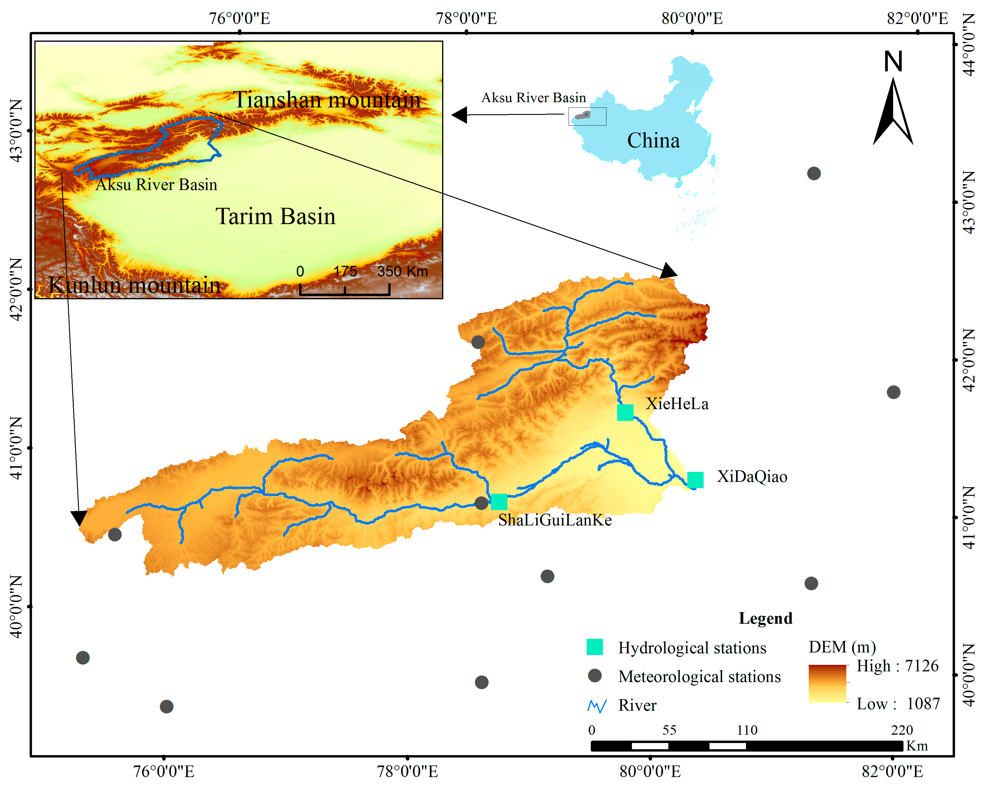
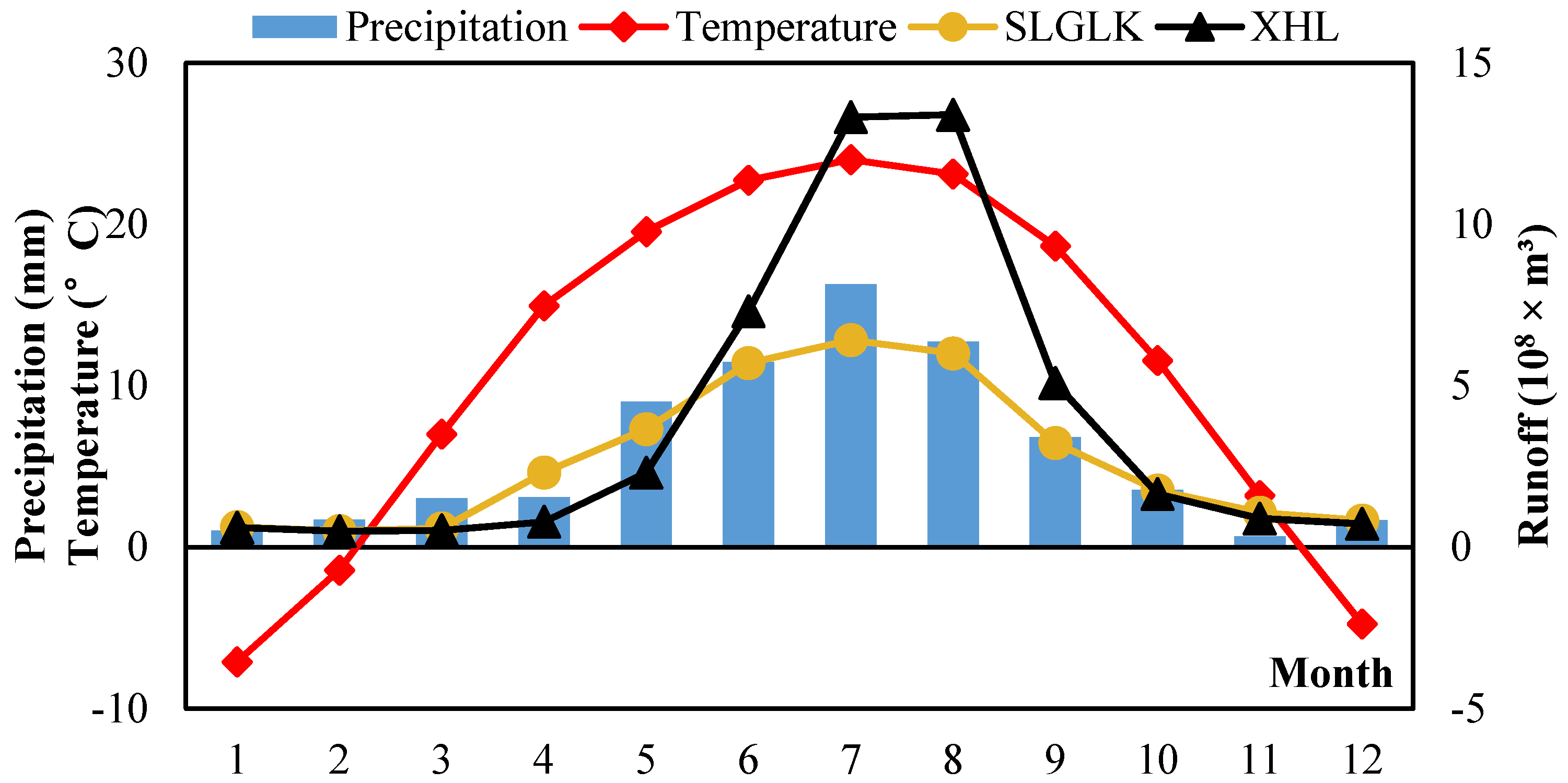
2.1. Study Area

The Aksu River Basin is located in the middle of the Tianshan Mountains (Figure 1) and converges into the Tarim River (75°3′–80°19′ E, 40°15′–42°30′ N). The elevation ranges between 1087 and 7126 m. The basin has an area of 4.3 × 10⁴ km² and as the terrain gradually descends from the north to the south and from the west to the east, it shows distinct geomorphological zones. Bare land and low-coverage grassland are the major land use/cover types in the Aksu River Basin and Leptosols, Fluvisols and Cambisols are the main soil types. Oases have a warm temperate continental arid climate controlled by the North Atlantic Oscillations, the variations of which can cause changes in the North Atlantic circulation system and the westerly trough and ridge system [53]. This basin has strong evaporation and large daily and yearly temperature differences. At the Aksu station (elevation of 1000 m), the annual average temperature is about 11 °C and the annual rainfall is around 71.09 mm. With the significant mountain effect at Tuergate station with an elevation of 3500 m, the annual average temperature falls down to −2.87 °C and the annual rainfall reaches 176.31 mm. The average monthly rainfall and temperature in the Aksu River basin are shown in Figure 2. Two major tributaries, the Kunmalike River and the Tuoshigan River, originate in Kyrgyzstan and converge at Kaladuwei. The average monthly runoff at each flume station is shown in Figure 2. Runoff in the mountainous regions is mainly caused by precipitation and snowmelt and the plains oasis regions are the major areas of water dissipation because of agricultural irrigation and ecological water consumption. The remaining water flows down to the Tarim River.

Xiehela station (XHL) and Shaliguilanke station (SLGLK) are located on the Kunmalike and Tuoshigan rivers, respectively. Xidaqiao station (XDQ) is at the confluence of two tributaries of the main stream of the Aksu River. Over the last 50 years, the LUCCs above the mountain outlet have been limited [54]. The area between the mountain outlet and Xidaqiao station at the piedmont plain has experienced human activities consisting of significant expansion of the cultivated land area (Figure 3). Subsequently, the Tarim River has obviously been affected by the inflow of the Aksu River [56].

2.2. Dataset

The annual discharge data from 1960 to 2011 at the XHL, SLGLK and XDQ hydrological stations were obtained from the Xinjiang Tarim River Basin Management Bureau. The daily discharge data from 2002 to 2007 were applied to calibrate the SWAT model.

Meteorological data including precipitation, temperature and other data, were acquired from the China Meteorological Data Sharing Service System (http://data.cma.cn/). Only one meteorological station is located in the basin and so it cannot represent the spatial distribution of the entire watershed. Therefore, the surrounding 12 stations (including one above 3000 m, two at approximately 2000 m and the remainder between 1000 and 2000 m) involved in this study were redistributed by Ordinary Kriging interpolation to generate 52 annual rainfall maps. The spherical method is selected for the parameter of semivariogram model and the search radius is set to 12 points. Changes in evaporation were used to reflect temperature changes. To select a suitable method of accurately calculating the PET in the mountainous area with little data [57], this study used the temperature-based Hargreaves equation [58], which requires less input data. The Hargreaves equation is as follows:

$$\text{PET}=0.0023\times Ra\times [\frac{T_{\text{max}}-T_{\text{min}}}{2}+17.8]\times {(T_{\text{max}}-T_{\text{min}})}^{0.5}$$

(1)

where $Ra$ is the extra-terrestrial radiation (MJ/m²/day), which can be acquired from the reference table [59]; $T_{\text{max}}$ is the mean maximum temperature in °C; and $T_{\text{min}}$ is the mean minimum temperature in °C. The spatial distribution maps of the annual PET were redistributed to produce an annual rainfall map.

The LUCC can characterize significant changes in the surface coverage caused by intense human activity or extreme natural events. In this study, the LUCC data from the 1960s, 1990, 2013 were generated based on topographic maps (1960s), Landsat MSS/TM and Landsat 8 products, the data were obtained from the Key Laboratory of Remote Sensing and Geographic Information System, the Xinjiang Institute of Ecology and Geography, Chinese Academy of Sciences. The data for the population, the cultivated area, the quantity of livestock and all types of agricultural product outputs were derived from statistical yearbooks, including “Fifty years in Xinjiang” [60] and the “Xinjiang statistical yearbook” from 1965 to 2012 [61].

2.3. Methods

This study used the non-parametric Mann-Kendall test [62,63] accumulative anomaly method [64], SCRCQ method [16,23], SWAT hydrological model [65,66,67] and Pearson correlation analysis [68]. The first two methods were used to identify any abrupt changes in the annual FDV from 1960 to 2011 because the combination of the two methods facilitated the accurate and comprehensive identification of break points [23,51]. The SCRCQ and SWAT model were used to perform a quantitative evaluation of the contributions of climate factors and human activities to the annual runoff variations. The Pearson correlation analysis was used to detect relevant simultaneous relationships between independent and dependent variables. The SCRCQ method and the Pearson correlation analysis method were used to determine the relationship between an independent and dependent variable, although the methods have different focuses.

2.3.1. Non-Parametric Mann-Kendall Test

The non-parametric Mann-Kendall test method [62,63] (M-K test) was used to analyse the trends in the long-term meteorological and hydrological series data, including rainfall, runoff, etc. This method does not require a sample to conform to a particular statistical distribution. Moreover, it is not affected by a small number of outliers and is especially suitable to non-normal distributed datasets such as climate and hydrological data.

The original null hypothesis H₀ of the M-K test is that the data in time series (X₁, …, X_n) are independent and identically distributed random variables; the hypothesis H₁ is that bilateral inspection of all of k, j ≤ n, and k ≠ j will show that the distribution of X_k and X_j are different. The test statistic S is calculated as follows:

$$S={\displaystyle \sum }_{k=1}^{n-1}{\displaystyle \sum }_{j=k+1}^{n}Sgn\left(X_j-X_k\right)$$

(2)

$$Sgn\left(X_j-X_k\right)=\{\begin{array}{c}+1 \left(X_j-X_k\right)>0 \\ 0 \left(X_j-X_k\right)=0\\ -1 \left(X_j-X_k\right)<0\end{array}$$

(3)

where S is normally distributed with a mean of 0.

$$V_a\left(\mathrm{S}\right)=n\left(n-1\right)\left(2n+5\right)/18$$

(4)

When n > 0, the standard normal distribution system variable is calculated by the following formula:

$$Z=\{\begin{array}{c}\frac{S-1}{\sqrt{V_a\left(S\right)}} S>0\\ 0 S=0\\ \frac{S+1}{\sqrt{V_a\left(S\right)}} S<0\end{array}$$

(5)

If a bilateral trend inspection at a given level of confidence indicates that $\left|Z\right|\ge Z_{1-a/2}$, then the null hypothesis is unacceptable at that confidence level and a significant upward or downward trend occurs in the time-series data. A value of statistic Z greater than 0 indicates a rising trend and a value less than 0 implies a downward trend. If the absolute value of Z is greater than or equal to 1.28, 1.64 and 2.32, the samples pass the significance test at confidence levels of 90%, 95%, and 99%, respectively.

It is recommended that the data series should be serially independent before applying the M-K test. Hydrological time series often exhibit statistically significant serial correlation. Therefore, the pre-whitening process was applied to detect serial correlation according to Yue and Wang (2002) [69]. The specific steps are as follows:

The lag-1 serial correlation coefficient $r_1$ is computed, and under the confidence level of $\mathsf{\delta }$, bilateral inspection is used to determine the significance of $r_1$:

$$r_1=\frac{\frac{1}{n-1}{\sum }_{i=1}^{n-1}[x_i-E\left(x_i\right)][x_{i+1}-E\left(x_i\right)]}{\frac{1}{n}{\sum }_{i=1}^n{[x_i-E\left(x_i\right)]}^2}$$

(6)

$$E\left(x_i\right)=\frac{1}{n}{{\displaystyle \sum }}_{i=1}^n{x}_i$$

(7)

$$\frac{-1-Z_{1-\mathsf{\delta }/2}\sqrt{n-2}}{n-1}\le r_1\le \frac{-1+Z_{1-\mathsf{\delta }/2}\sqrt{n-2}}{n-1}$$

(8)

where $r_1$ is the lag-1 serial correlation coefficient of sample data $x_i$, $E\left(x_i\right)$ is the mean value of sample data. The lag-1 autoregressive AR(1) is removed from $x_i$ by

$$y_i=x_i-r_1{x}_{i-1}$$

(9)

The M-K test is applied to the processed data series to assess the significance of the trend after pre-whitening process.

The M-K test can be further applied and a different test statistic from Z can be calculated by constructing a column order:

$$S_k={\displaystyle \sum }_{i=1}^k{\displaystyle \sum }_j^{i-1}{a}_{ij} \left(k=2,3,4,···,n\right)$$

(10)

$$a_{ij}=\{\begin{array}{c}1 X_i>X_j\\ 0 X_i<X_j\end{array} 1\le j\le i$$

(11)

The statistical variables are as follows:

$$U{F}_k=\frac{[S_k-E\left(S_k\right)]}{\sqrt{V_{ar}\left(S_k\right)}} \left(k=1,2,···,n\right),$$

(12)

$$E\left(S_k\right)=\frac{k\left(k+1\right)}{4}$$

(13)

$$V_{ar}\left(S_k\right)=k\left(k-1\right)\left(2k+5\right)/72$$

(14)

where $U{F}_k$ is the standard normal distribution. For a specific level of significance $a$, if $\left|U{F}_k\right|\ge U_{a/2}$, then a clear trend occurs in the sequence. Arranging the time series of x in reverse order and performing the corresponding calculation produces the following:

$$\{\begin{array}{c}U{B}_k=-U{F}_k\\ k=n+1-k\end{array} \left(k=1,2,···,n\right)$$

(15)

By combining the statistical series $U{F}_k$ and $U{B}_k$, the trends in x and the break point can be clearly identified. If $U{F}_k$ is greater than 0, then the sequence exhibits a rising trend and if $U{F}_k$ is less than 0, then a downward trend is indicated. When the values exceed the critical straight line, then a significant upward or downward trend is indicated. If the $U{F}_k$ and $U{B}_k$ curves appear at an intersection and fall in between the critical straight lines, then intersection indicates a break point at which the trends change.

2.3.2. Accumulative Anomaly Method

The accumulative anomaly method [64] is a statistical method for intuitively judging the change in a trend of discrete data points by a curve. The difference in the average value of the annual runoff is first calculated and then chronologically accumulated to obtain a changing process that shows the accumulative anomaly over time. In the drawing process, the data for the cumulative anomaly sequences were normalized to facilitate the presentation of the results; thus the cumulative anomaly sequences were divided by the perennial average value of the runoff. If the cumulative anomaly value was higher, then the discrete data were larger than average and showed an increasing trend and if the anomaly value was lower, then the data were smaller than average and showed a decreasing trend. The inflection points are the break points.

2.3.3. SCRCQ

The principle of the improved SCRCQ method [12,28] is that if the runoff variation is only affected by precipitation, then the slope of the linear relationship between the yearly and cumulative precipitation and the cumulative runoff will change at the same rate. This method assumes that the slope of the linear relationship between the yearly and cumulative runoff before and after a year of break point is $S_{Rb}$ and $S_{Ra}$ (10⁸ m³/a), respectively. The rate of change in the slope of the cumulative runoff can be expressed as follows:

$$S{C}_R=\frac{S_{Ra}-S_{Rb}}{S_{Rb}}$$

(16)

The slopes of the linear relationship between the yearly and cumulative precipitation before and after the years of break points are $S_{Pb}$ and $S_{Pa}$ (mm/a) respectively. The rate of the change in the slope of the cumulative precipitation can be expressed as follows:

$$S{C}_P=\frac{S_{Pa}-S_{Pb}}{S_{Pb}}.$$

(17)

Therefore, the contribution of precipitation ($C_P$, unit: %) to the runoff variations before and after the year of break points can be expressed as follows:

$$C_P=100\times S{C}_P/S{C}_R$$

(18)

Similarly, the slopes of the linear relationship between the yearly and the cumulative potential evapotranspiration before and after the year of break points are represented by $S_{Eb}$ and $S_{Ea}$ (mm/a) respectively. The rate of change in the slope of the cumulative PET can be expressed as follows:

$$S{C}_E=\frac{S_{Ea}-S_{Eb}}{S_{Eb}}$$

(19)

Therefore, the contribution of the PET ($C_E$, unit: %) to the runoff variations before and after the year of break point scan be expressed as follows:

$$C_E=-100\times S{C}_E/S{C}_R$$

(20)

Based on the water balance, the contribution of human activities ($C_H$, unit: %) to the runoff variations can be expressed as follows:

$$C_H=100-C_P-C_E-C_G$$

(21)

where $C_G$ is the contribution of the groundwater to the runoff variations ($C_G$, unit: %). Because the headwater mainly originates from alpine glacier melt/snowmelt, the rocky geo-structure barely generates the massive groundwater flow in the upstream region. However, streams in the downstream valley and plain area are primarily recharged by rainfall, melt water and groundwater, and activities that exploit the groundwater occur in the farmlands in the downstream region. Thus, the effect of groundwater on runoff variations above the mountain outlets can be ignored, although the effect below plain streams is considered the result of human activities [49]. Therefore, the factors that affect runoff variations (Equation (21)) can be simplified to

$$C_H=100-C_P-C_E$$

(22)

2.3.4. Soil and Water Assessment Tool (SWAT Model)

For this study, a semi-distributed hydrological model, the Soil & Water Assessment Tool (SWAT model) [65], which has been demonstrated as appropriate for numerous worldwide watersheds [66,67], was used to evaluate the effects of climate change and LUCC on hydrological processes. The hydrological components simulated by the SWAT model include evapotranspiration (ET), surface runoff, percolation, lateral flow, groundwater flow, transmission losses, etc. [70]. SWAT input data requirements include a digital elevation model (DEM), meteorological records, soil characteristics, land use/cover classification and management schedules for key land uses (pastoral farming, wastewater irrigation, timber harvesting, etc.). Descriptions and sources of the data used to configure the SWAT model are given in

Table 1. Description of Data Used to Configure the SWAT Model.

Data	Application	Data Description and Configuration Details	Source
Digital Elevation Model (DEM)	Sub-basin delineation and stream network extraction	Data at 90 m resolution; used to define four slope classes: 0%–25%, 25%–45%, 45%–65% and >65%.	Shuttle Radar Topography Mission (SRTM)
Land use/cover	HRU definition	Vector data; 12 basic land use/cover categories.	Key Laboratory of Remote Sensing and Geographic Information System, Xinjiang Institute of Ecology and Geography, Chinese Academy of Sciences
Soil characteristics	HRU definition	1 km resolution, 15 soil types.	Food and Agriculture Organization (FAO), Harmonized World Soil Database version 1.1 (HWSD)
Meteorological data	Meteorological forcing	Daily maximum and minimum temperature, daily precipitation.	China Meteorological Data Sharing Service System
Hydrological observation data	Calibration and validation	Daily observation runoff data of SLGLK and XHL.	Tarim River Basin Management Bureau

. The daily discharge was calibrated and validated based on the daily values of the SLGLK and XHL measurements. In addition, the operational regime for wastewater irrigation and auto-irrigation has been considered in the SWAT model. The sensitive parameters of SWAT model were identified by automated Latin Hypercube One-factor-At-a-Time (LH-OAT) [71] global sensitivity analysis procedures and the uncertainty of calibrated values was estimated with automated methods based on the Sequential Uncertainty Fitting (SUFI-2) [72] algorithm (

Table 2. Sensitivity Rate, Calibration Range, Subbasin and Final Calibration Estimate of Top Ten Selected SWAT Model Parameters.

Component	Parameter Name	Sensitivity Rate	Calibration Range	Subbasin	Final Estimate
Basin/snow	SFTMP	4	−5~5	Share	−0.552
	SMTMP	1	−5~5	Share	−0.2478
	SMFMX	7	0~10	Share	6.8002
	SMFMN	10	0~10	Share	1.5104
	TIMP	8	0.01~1	Share	0.0873
	PLAPS	2	0~500	SLGLK	70
				XHL	280
	TLAPS	3	−10~10	SLGLK	−6.5
				XHL	−4.5
Surface runoff	LAT_TTIME	5	0~180	SLGLK	7
				XHL	3
	CH_K2	9	0~500	SLGLK	0.006
				XHL	0.65
Ground water	ALPHA_BF	6	0~1	SLGLK	0.5
				XHL	1

). The calibration period was from 2002 to 2004 and the validation period was from 2005 to 2007. The Nash–Sutcliffe efficiency (NSE) values for the SLGLK discharge were 0.647 for calibration and 0.624 for validation, and the NSE values for the XHL discharge were 0.647 for calibration and 0.620 for validation; thus, the model performed well.

To analyse the effects of climate change and human activities on the FDV using the model, three scenarios were designed. Scenario 1 (S1) used climate records and a land use/cover map from before the year of break point as the baseline. The climate records and land use/cover map after the year of break points were applied in Scenario 2 (S2), which reflects the combined effect of climate change and human activities on the FDV. In Scenario 3 (S3), the climate records after the year of break points were replaced without changing the land use/cover map. Differences in the FDV of S2 and S1 ($D_t$) were considered the total combined impact of climate change and human activities on the FDV. The effects of climate change and human activities were calculated by the difference in the FDV between S3 and S1 ($D_c$) and the difference in the FDV between S2 and S3 ($D_h$), respectively. Therefore, the contribution of the impact of climate change on the FDV ($C_c$) can be expressed as follows:

$$C_c=\raisebox{1ex}{$D_c$}\!\left/ \!\raisebox{-1ex}{$D_t$}\right.$$

(23)

The contribution of the impact of human activities on the FDV ($C_h$) can be expressed as follows:

$$C_h=\raisebox{1ex}{$D_h$}\!\left/ \!\raisebox{-1ex}{$D_t$}\right.$$

(24)

2.3.5. Pearson Correlation Analysis

The Pearson correlation analysis [68] is commonly used to analyse the relationship between two random variables or two datasets. Pearson’s correlation coefficient is a measure of the relationship between two mathematical variables or measured data values. In this study, this coefficient was used to analyse the correlation between the annual FDV, the temperature and precipitation in the Aksu River Basin. The formula for Pearson’s correlation coefficient is as follows:

$$r=\frac{N{\sum }^{\text{}}{x}_i{y}_i-{\sum }^{\text{}}{x}_i{\sum }^{\text{}}{y}_i}{\sqrt{N{\sum }^{\text{}}{x}_i^2-{({\sum }^{\text{}}{x}_i)}^2}\sqrt{N{\sum }^{\text{}}{y}_i^2-{({\sum }^{\text{}}{y}_i)}^2}}$$

(25)

where $r$ is Pearson’s correlation coefficient and $x_i$ and $y_i$ are the values of two target datasets. The correlation coefficient is between −1 and 1 and values of +1 indicate a perfect direct (increasing) linear relationship (correlation), whereas values of −1 indicate a perfect decreasing (inverse) linear relationship (anticorrelation). When the value approaches zero, there is less of a relationship (closer to uncorrelated). A coefficient value closer to either −1 or 1 indicates a stronger correlation among the variables [73].

2.3.6. Agricultural Water Footprint

The agricultural water footprint refers to the volume of water consumed by the growth of agricultural products (broad irrigation is the principal irrigation method) and it can reflect the actual volume of water used for agriculture [74]. The agricultural water footprint can be calculated by multiplying the various agricultural output values by the associated virtual water content (VWC) and then summing, which is expressed as follows:

$$WF={\displaystyle \sum }_{i=1}^n(P_i\times VW{C}_i)$$

(26)

where $WF$ denotes the total agricultural water footprint (m³), $P_i$ denotes the agricultural output (kg) and $VW{C}_i$ denotes the virtual water content (m³/kg), which is defined as the volume of water required to produce the agricultural products. Three types of agricultural products have been considered in this study: food crops (rice, wheat, maize, beans, etc.), commercial crops (oil plants, beet, fruits, vegetable, etc.) and animal products (meat, etc.). Based on related studies [74,75] and the conditions on the ground in the Aksu River Basin, the VWC of all agricultural products types are listed in

Table 3. Unit Factors for the Virtual Water Footprint of the Primary Farm Products in the Aksu River Basin.

Agricultural Products	Food Crops	Commercial Crops					Animal Products
		Cotton	Oil Plants	Beet	Vegetable	Fruits	Meat
Unit Factor/(m3/kg)	1.532	3.871	2.74	0.171	1.152	1.152	5.91

. The VWC of the food crops and commercial crops are composed of the rainfall and irrigation volume for crop growth. The VWC of the animal products is primary physiological water requirements and is not double counted with the VWC of food crops because most animals feed on alfalfa.

3. Results and Discussion

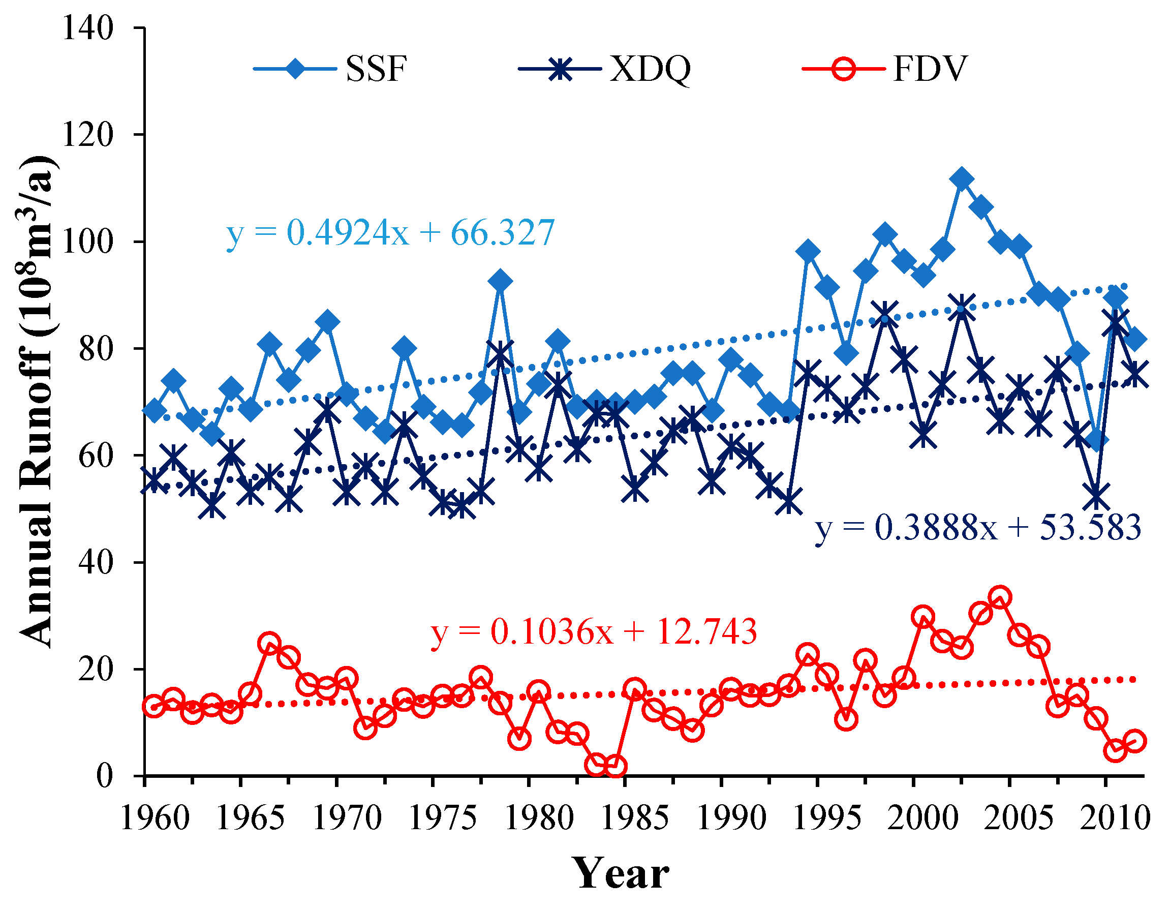
3.1. Changes and Trends in Annual Runoff

To quantify the long-term trends at key points in the basin, the sum of the source flow (SSF), Xidaqiao (XDQ) and flow difference value (FDV) were calculated for the period from 1960 to 2011. All of the variables showed a clear increasing trend (Figure 4). According to the slopes of the trend lines, the SSF showed the most pronounced increase (p-value < 0.001), XDQ showed a moderate increase (p-value < 0.001) and the FDV only showed a small increase (p-value = 0.101). Although the values for the source regions showed similar increasing trends compared with the basin outlet, the rates at the source regions increased more rapidly. In addition, the annual fluctuation of the SSF runoff and the XDQ runoff were relatively small and synchronized. The coefficients of variation (Cv) of the annual runoff were 0.160 and 0.155. However, the annual fluctuation of the FDV was relatively large and the Cv reached 0.44. Thus the FDV appeared to present greater variability when compared with the SSF and XDQ.

Applying a linear trend analysis to the annual runoff at all stations revealed a trend of increasing volatility at values of 0.49 × 10⁸ m³/a, 0.39 × 10⁸ m³/a and 0.10 × 10⁸ m³/a, which indicated that the increasing runoff rate gradually reduces along the streams.

3.2. Mutation Analysis

Because the non-parametric Mann-Kendall test and accumulative anomaly method do not require the samples to conform to a particular statistical distribution function, it is easy to identify the year of break points. Both the M-K test and the accumulative anomaly method were used in this study after pre-whitening process to analyse the break point of the FDV. Figure 5a shows that the annual FDV appeared to mutate in 1965, 1969 and 1988 but in 1965 and 1988 were within the 95% confidence interval. Figure 5b shows that the annual FDV appeared to mutate in 1965, 1967, 1988 and 2006 and in 1965 and 1988 were consistent with the results of the M-K test. Although there is an intersection in the M-K test in 1969, the point is outside the 95% confidence interval. In addition, evidence of a year of break point is not observed in 1967 and 2006 using the M-K test, thus 1967 and 2006 cannot be considered to be the break points. Because both the M-K test and the accumulative anomaly method confirmed that 1965 and 1988 are the break points for FDV changes, the entire study period was divided into three stages: stage (I), 1960–1965; stage (II), 1966–1988 and stage (III), 1989–2011.

Previous research results [50,51,55] indicated that the annual runoff in the early 1990s reflect the year of break points in the Aksu River Basin. However, because different methods and target variables were employed, a clear year of break point was not evident. In this study, the year of break point of the FDV was indicated by both the non-parametric M-K test and the accumulative anomaly method as 1988. Therefore, this study focused on stages II and III to analyse the contribution of each factor to the changes in the FDV. Stage I was omitted because the time span was relatively short and did not show clear statistical properties.

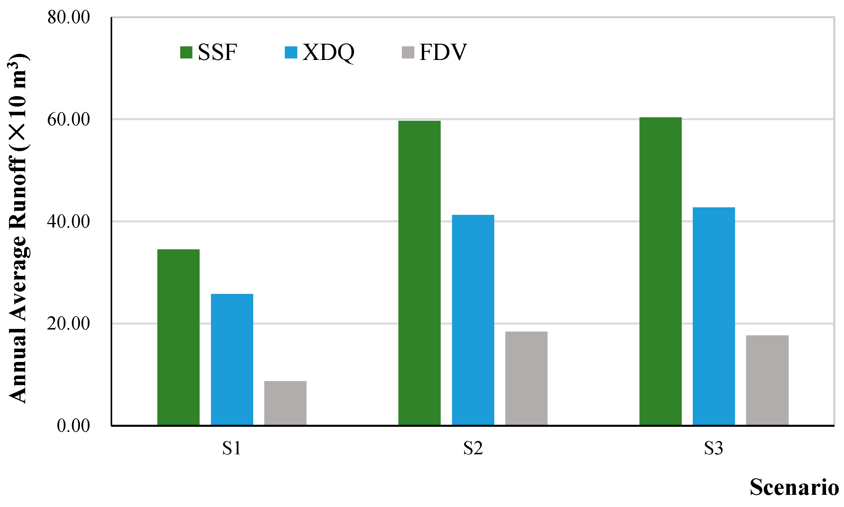
3.3. Contributions of Driving Factors to Changes in the FDV

3.3.1. SCRCQ Method

Based on the year of break point, a linear regression analysis was conducted for the cumulative time series of the FDV (Figure 6a), precipitation (Figure 6b) and PET (Figure 6c) and the resulting coefficients of determination (R²) of the regression equations were greater than 0.983, 0.988 and 0.999 respectively, with p-values that were far less than 0.001. Furthermore, Figure 6 and equations 16, 17, and 19 indicate that the rate of change of the slope of the cumulative runoff, precipitation and PET are 72.24%, 55.87% and 0.71% respectively. The rate of change of the slope for the FDV was greater than that for precipitation and PET, which indicates that the changes in FDV were impacted by other factors, which we attribute to human activities. The contributions of precipitation, PET and human activities to the changes in the FDV were calculated based on the variables listed in

Table 4. Slope Change Ratios of the Fitted Lines and the Quantitative Impacts of Precipitation, PET and Human Activities on FDV Variations During Different Periods.

Time Period	${\mathit{S}}_{\mathit{R}}$(108 m3/a)	${\mathit{S}}_{\mathit{P}}$(mm/a)	${\mathit{S}}_{\mathit{E}}$(mm/a)	${\mathit{C}}_{\mathit{P}}$(%)	${\mathit{C}}_{\mathit{E}}$(%)	${\mathit{C}}_{\mathit{H}}$(%)
II	12.09	120.52	2409.1	-	-	-
III	20.83	187.86	2426.2	77.35	−0.98	23.63

, which indicates that the changes in the FDV were impacted by climate factors and human activities in stage III.

The contributions of precipitation, PET and human activities to the changes in the FDV were calculated by the SCRCQ and they are listed in Table 4. Compared with stage II, the scale of the effect of precipitation, PET and human activities on the changes in FDV was 77.35%, −0.98% and 23.63%, respectively. This result shows that precipitation was the most important factor, followed by human activities and PET, which had the least effect. The driving factor that produced the largest contribution was precipitation, which presented a significantly increasing trend in Xinjiang as a result of climate change [76,77]. Thus, the slope change ratio of the cumulative FDV is similar to the slope change ratio of the accumulative precipitation and considerably different than the slope change ratio of the cumulative PET (Figure 6c). The method of calculating the PET does not reflect changes in the natural properties of the watershed; therefore the contribution of the PET to the FDV is reduced. The possibility of human activities having a substantial contribution to the slope change ratio of the cumulative FDV is appreciable. The lower Aksu River Basin is flat and a large amount of land has been reclaimed for massive irrigation cultivation, including paddy fields. Therefore, a large amount of water has been consumed in this region [8] which has affected the slope change ratio of the cumulative FDV. Moreover, the contribution of the driving factors to the actual change of the annual runoff difference varies with the amount of total runoff.

3.3.2. Model Simulation Method

The SSF, XDQ and FDV for the three scenarios were investigated using the SWAT model (Figure 7). With respect to the year of break point, the annual average runoff of the SSF was 34.51 × 10⁸ m³, 59.71 × 10⁸ m³ and 60.39 × 10⁸ m³. The SSF of S2 had a similar volume to that of S3 because the runoff from the mountain outlet was not used for irrigation. However, the water runoff of XDQ was different in the three scenarios and presented values of 28.21 × 10⁸ m³, 44.12 × 10⁸ m³ and 45.72 × 10⁸ m³. Human activities, especially irrigation, caused the runoff of XDQ in S2 to be lower than that in S3. Therefore the FDV of S2 was larger at 18.43 × 10⁸ m³. The FDV of S1 and S3 was 8.71 × 10⁸ m³ and 17.68 × 10⁸ m³, respectively.

The contributions of climate change and human activities were calculated for each scenario as described in Section 2.3.4. The contribution percentages of climate change and human activities were 92.28% and 7.72%, respectively. An increase in precipitation and temperature related to climate change causing additional rainfall and snowmelt in Xinjiang [44,76]. The expansion of arable land caused by human activities led to an increase in the irrigation volume, which decreased the runoff of XDQ [8]. The results again suggest that the effect of climate change on the FDV is higher than that of human activities.

The results of the two calculation methods used to determine the contributions of climate change and human activities on the FDV are consistent and yield similar results for the effects of climate change on the FDV. Moreover, the results indicate that the effects of climate change were greater than the effects of human activity. However, the contribution of climate change indicated by the SCRCQ method is less than that indicated by the SWAT model and the contribution of human activity indicated by the SCRCQ method is greater than that indicated by the SWAT model. Because the SWAT model considers precipitation as well as temperature, relative humidity and many other variables, it can properly reflect the inter-relationships between temperature and increased snowmelt volumes [34]. However, it is difficult to consider temperature using the SCRCQ method. Therefore, the contribution percentage of the impact of climate change on runoff indicated by the SWAT model is higher than that indicated by the SCRCQ method.

3.4. Climate Change Factor

Climate change directly affects the mountain outlet runoff through its effects on temperature and precipitation [78,79]. Relevant research data show that for most mountain regions, the annual runoff and the annual precipitation and temperature are consistent [80,81]. However, few studies have focused on the relationship of the FDV with climate factors. The Aksu River consists of the Tuoshigan River and Kunmalike River, which show runoff variations that are influenced by precipitation, temperature, glacier/snow cover area and other related factors [51]. Correlation analyses and the regression coefficient method combined with pre-whitening process were used to investigate the changes in the FDV for the Aksu River and determine whether those changes had a close relationship with meteorological elements.

The Aksu River is supplied by mountain glacier/snow melt water; therefore, runoff variations are affected by temperature and precipitation. However, whether the change in the FDV is related to temperature and precipitation is unclear, thus the Pearson correlation method was used to investigate the relationship. The analysis results are shown in

Table 5. Correlation Coefficient Between the Annual FDV and Temperature and Precipitation in the Aksu River Basin.

Climate Factors	Stage II		Stage III
	Annual Mean Temperature	Annual Precipitation	Annual Mean Temperature	Annual Precipitation
Annual FDV	0.024	–0.272	0.082	–0.472

, which show that in stage II, the correlation coefficient between the annual FDV and the annual mean temperature is 0.024 and the correlation coefficient between the annual FDV and the annual precipitation is −0.272. In stage III, the correlation coefficient between the annual FDV and the annual mean temperature is 0.082, and the correlation coefficient between the annual FDV and the annual precipitation is −0.472. These results were not significant.

The FDV, temperature and precipitation data were normalized and the three regression equations were recalculated for the same period with the following results:

$$\text{stage II}:Y=-0.02809X_1+0.04951X_2+8.41318,\text{ Sig}.=0.4822>0.05,\text{ non}-\text{significant}$$

$$\text{stage III}: Y=-0.06267X_1-0.20857X_2+20.96526,\text{ Sig}.=0.0912>0.05,\text{ non}-\text{significant}$$

where $Y$ is the annual FDV; $X_1$ is the annual precipitation; and $X_2$ is the annual mean temperature.

The above two regression equations were not significant at the 95% level. The results showed a non-linear relationship between the climate change factors and the FDV. Therefore, the relationship must be calculated by hydrological models in a future study.

3.5. Human Activity Factor

The previous results showed that human activities had a significant impact on the FDV. The population, sown area, livestock quantity, agricultural water footprint and cultivated land areas were included in this study in Wensu and Wushi Counties in the Aksu River Basin.

A higher correlation was found between the FDV and agricultural water footprint with a correlation coefficient of 0.51 (Figure 8). Moreover, the p-values were less than 0.01, which showed that the relationship between the FDV and the agricultural water footprint was important. There were weak, non-significant correlations between FDV and population, sown area and livestock quantity. Agricultural water footprint change can reflect changes in sown area, livestock quantity, and other factors [63]. The construction land area and the effective irrigation area have increased to varying degrees due to rapid population growth and the accelerated urbanization process in the Aksu River Basin [8,54]. Statistics indicate that the basin population has increased from 179,600 in 1955 to 463,200 in 2011, with accelerated development occurring in the early 1980s. In addition, grazing in the basin has become more developed, with livestock quantities increasing from 468,800 in 1955 to 1,104,800 in 2011, a more than 2-fold increase. Unjustifiable human activities such as over grazing has caused a degradation and reduced ability of the earth’s surface to retain rainfall-runoff, thereby accelerating the loss of water and soil [82].

In addition, the expansion of cultivated land area was the most obvious factor related to human activities that has affected the runoff in the Aksu River Basin [52] and it has primarily occurred on both sides of the river downstream (Figure 3). The cultivated land area increased from 965.87 km² in the 1960s to 1113.16 km² in 1990 and to 1347.67 km² in 2013. From the 1960s~1990, the cultivated land area increased by approximately 4.91 km²/a, whereas from 1990 to 2013, the cultivated land area rapidly expanded to 10.20 km²/a (

Table 6. Expansion of Cultivated Land in the Oasis Area of the Aksu River Basin.

Year	Area (km2)	Increment (km2)	Increased Proportion (%)	Increased Speed (km2/a)
1960s	965.87	-	-	-
1990	1113.16	147.29	15.25	4.91
2013	1347.67	234.51	21.07	10.20

).

4. Conclusions

Climate change together with human activities showed vital influences on mountainous stream runoff. The recorded runoff of SSF and XDQ in the study area presented significantly increasing trends with linear increasing rates of 0.49 × 10⁸ m³/a and 0.39 × 10⁸ m³/a respectively, while the FDV expressed non-significant increasing trend. An abrupt change in the FDV series was detected in 1965 and 1988 using a pre-whitening M-K test and accumulative anomaly method. The approach of using the pre-whitening process eliminates the autocorrelation among the data series which might severely mislead analysis direction and cause a potential bias. The year 1988 was taken as the break point for the contribution analysis.

Although climate plays a crucial impact on the change of FDV, the influence exercised by human activities cannot be ignored during the contribution analysis. The contribution of climate change and human activities on FDV for the period of 1988–2011 were 76.37% and 23.63% calculated by SCRCQ, and were 92.28% and 7.72% by SWAT. Climate change and human activities exert lasting impacts on FDV for the whole study period, but the agricultural water footprint influence under human activities was clearly apparent after the break point. Although the SCRCQ method considered the quantities of precipitation, evapotranspiration and human activities, the hydrological processes and other climate variables were neglected in this statistical analysis, while the modelling approach might have the detailed consideration for all the possible driving factors. Therefore, it is pivotal to take climate change and human activities into account by multiple analysis approaches on water resources management as well as ecological restoration.

References

1. Törnqvist, R.; Jarsjö, J.; Pietroń, J.; Bring, A.; Rogberg, P.; Asokan, S.M.; Destouni, G. Evolution of the hydro-climate system in the lake baikal basin. J. Hydrol. 2014, 519, 1953–1962. [Google Scholar] [CrossRef]
2. Ohana-Levi, N.; Karnieli, A.; Egozi, R.; Givati, A.; Peeters, A. Modeling the effects of land-cover change on rainfall-runoff relationships in a semiarid, eastern mediterranean watershed. Adv. Meteorol. 2015, 2015, 1–16. [Google Scholar] [CrossRef]
3. Ljungqvist, F.C.; Krusic, P.J.; Sundqvist, H.S.; Zorita, E.; Brattstrom, G.; Frank, D. Northern hemisphere hydroclimate variability over the past twelve centuries. Nature 2016, 532, 94–98. [Google Scholar] [CrossRef] [PubMed]
4. Miao, L.; Jiang, C.; Xue, B.; Liu, Q.; He, B.; Nath, R.; Cui, X. Vegetation dynamics and factor analysis in arid and semi-arid inner mongolia. Environ. Earth Sci. 2014, 73, 2343–2352. [Google Scholar] [CrossRef]
5. Mahmoud, S.H.; Alazba, A.A. Hydrological response to land cover changes and human activities in arid regions using a geographic information system and remote sensing. PLoS ONE 2015, 10, e0125805. [Google Scholar] [CrossRef] [PubMed]
6. Abu-Allaban, M.; El-Naqa, A.; Jaber, M.; Hammouri, N. Water scarcity impact of climate change in semi-arid regions: A case study in mujib basin, jordan. Arab. J. Geosci. 2014, 8, 951–959. [Google Scholar] [CrossRef]
7. Liu, T.; Fang, H.; Willems, P.; Bao, A.M.; Chen, X.; Veroustraete, F.; Dong, Q.H. On the relationship between historical land-use change and water availability: The case of the lower tarim river region in northwestern china. Hydrol. Proc. 2013, 27, 251–261. [Google Scholar] [CrossRef]
8. Huang, S.; Krysanova, V.; Zhai, J.; Su, B. Impact of intensive irrigation activities on river discharge under agricultural scenarios in the semi-arid aksu river basin, northwest china. Water Res. Manag. 2014, 29, 945–959. [Google Scholar] [CrossRef]
9. Zhang, G.; Guhathakurta, S.; Lee, S.; Moore, A.; Yan, L. Grid-based land-use composition and configuration optimization for watershed stormwater management. Water Res. Manag. 2014, 28, 2867–2883. [Google Scholar] [CrossRef]
10. Zuo, Q.; Zhao, H.; Mao, C.; Ma, J.; Cui, G. Quantitative analysis of human-water relationships and harmony-based regulation in the tarim river basin. J. Hydrol. Eng. 2014, 20. [Google Scholar] [CrossRef]
11. Stocker, T.F.; Qin, D.; Plattner, G.-K.; Tignor, M.; Allen, S.K.; Boschung, J. IPCC 2013: Climate Change 2013: The Physical Science Basis. Contribution of Working Group I to the Fifth Assessment Report of the Intergovernmental Panel on Climate Change; Cambridge University Press: Cambridge, UK, 2013. [Google Scholar]
12. Kliment, Z.; Matoušková, M. Runoff changes in the šumava mountains (black forest) and the foothill regions: Extent of influence by human impact and climate change. Water Resour. Manag. 2008, 23, 1813–1834. [Google Scholar] [CrossRef]
13. Wang, D.; Hejazi, M. Quantifying the relative contribution of the climate and direct human impacts on mean annual streamflow in the contiguous united states. Water Resour. Res. 2011, 47, W00J12. [Google Scholar] [CrossRef]
14. Liu, Q.; Yang, Z.; Cui, B.; Sun, T. Temporal trends of hydro-climatic variables and runoff response to climatic variability and vegetation changes in the yiluo river basin, china. Hydrol. Proc. 2009, 23, 3030–3039. [Google Scholar] [CrossRef]
15. Chawla, I.; Mujumdar, P.P. Isolating the impacts of land use and climate change on streamflow. Hydrol. Earth Syst. Sci. Discuss. 2015, 12, 2201–2242. [Google Scholar] [CrossRef]
16. Wang, S.; Yan, M.; Yan, Y.; Shi, C.; He, L. Contributions of climate change and human activities to the changes in runoff increment in different sections of the yellow river. Quat. Int. 2012, 282, 66–77. [Google Scholar] [CrossRef]
17. Liu, T.; Willems, P.; Feng, X.W.; Li, Q.; Huang, Y.; Bao, A.M.; Chen, X.; Veroustraete, F.; Dong, Q.H. On the usefulness of remote sensing input data for spatially distributed hydrological modelling: Case of the tarim river basin in china. Hydrol. Proc. 2012, 26, 335–344. [Google Scholar] [CrossRef]
18. Stednick, J.D. Monitoring the effects of timber harvest on annual water yield. J. Hydrol. 1996, 176, 79–95. [Google Scholar] [CrossRef]
19. Liu, H.F.; Zhu, Q.K.; Sun, Z.F.; Wei, T.X. Effects of different land uses and land mulching modes on runoff and silt generations on loess slopes. Agric. Res. Arid Areas 2005, 23, 137–141. [Google Scholar]
20. Meginnis, H.G. Increasing Water Yields by Cutting Forest Vegetation. In Proceedings of the Symposium of Hannoversch-Munden, Gentbrugge, Germany, 8–14 September 1959; Publ. 48. International Association of Scientific Hydrology: Louvain, Belgium, 1959; pp. 59–68. [Google Scholar]
21. Burgy, R.H.; Papazafiriou, Z.G. Vegetative management and water yield relationships. In Proceedings of the 3rd International Seminar for Hydrology Professors, Purdue University, Lafayette, IN, USA, 18–31 July 1971.
22. Bosch, J.M.V.; Hewlett, J. A review of catchment experiments to determine the effect of vegetation changes on water yield and evapotranspiration. J. Hydrol. 1982, 55, 3–23. [Google Scholar] [CrossRef]
23. Wang, S.; Wang, Y.; Ran, L.; Su, T. Climatic and anthropogenic impacts on runoff changes in the songhua river basin over the last 56 years (1955–2010), Northeastern China. Catena 2015, 127, 258–269. [Google Scholar] [CrossRef]
24. Guo, J.; Zhang, Z.; Zhou, J.; Wang, S.; Strauss, P. Decoupling streamflow responses to climate variability and land use/cover changes in a watershed in Northern China. J. Am. Water Resour. Assoc. 2014, 50, 1425–1438. [Google Scholar] [CrossRef]
25. Chen, J.; Li, X. The impact of forest change on watershed hydrology—Discussing some controversies on forest hydrology. J. Nat. Res. 2000, 16, 474–480. [Google Scholar]
26. Zhang, X.; Zhang, L.; Zhao, J.; Rustomji, P.; Hairsine, P. Responses of streamflow to changes in climate and land use/cover in the Loess Plateau, China. Water Resour. Res. 2008, 44, W00A07. [Google Scholar] [CrossRef]
27. Zhang, C.; Zhang, B.; Li, W.; Liu, M. Response of streamflow to climate change and human activity in xitiaoxi river basin in China. Hydrol. Proc. 2014, 28, 43–50. [Google Scholar] [CrossRef]
28. Rust, W.; Corstanje, R.; Holman, I.P.; Milne, A.E. Detecting land use and land management influences on catchment hydrology by modelling and wavelets. J. Hydrol. 2014, 517, 378–389. [Google Scholar] [CrossRef]
29. Sun, W.-Y.; Bosilovich, M.G. Planetary boundary layer and surface layer sensitivity to land surface parameters. Bound. Layer Meteorol. 1996, 77, 353–378. [Google Scholar] [CrossRef]
30. Yao, Y.L.; Lv, X.G.; Wang, L. A review on study methods of effect of land use and land cover change on watershed hydrology. Wetl. Sci. 2009, 7, 83–88. [Google Scholar]
31. Liu, W.; Wei, X.; Liu, S.; Liu, Y.; Fan, H.; Zhang, M.; Yin, J.; Zhan, M. How do climate and forest changes affect long-term streamflow dynamics? A case study in the upper reach of poyang river basin ecohydrology early view. Ecohydrology 2014, 46–57. [Google Scholar] [CrossRef]
32. Baker, T.J.; Miller, S.N. Using the soil and water assessment tool (swat) to assess land use impact on water resources in an east African watershed. J. Hydrol. 2013, 486, 100–111. [Google Scholar] [CrossRef]
33. Memarian, H.; Balasundram, S.K.; Talib, J.B.; Teh Boon Sung, C.; Mohd Sood, A.; Abbaspour, K.C. Kineros2 application for land use/cover change impact analysis at the Hulu Langat basin, Malaysia. Water Environ. J. 2013, 27, 549–560. [Google Scholar] [CrossRef]
34. Santos, R.M.B.; Sanches Fernandes, L.F.; Moura, J.P.; Pereira, M.G.; Pacheco, F.A.L. The impact of climate change, human interference, scale and modeling uncertainties on the estimation of aquifer properties and river flow components. J. Hydrol. 2014, 519, 1297–1314. [Google Scholar] [CrossRef]
35. Cibin, R.; Athira, P.; Sudheer, K.P.; Chaubey, I. Application of distributed hydrological models for predictions in ungauged basins: A method to quantify predictive uncertainty. Hydrol. Proc. 2014, 28, 2033–2045. [Google Scholar] [CrossRef]
36. Wang, G.; Zhang, J.; Yang, Q. Attribution of runoff change for the xinshui river catchment on the Loess Plateau of China in a changing environment. Water 2016, 8, 267. [Google Scholar] [CrossRef]
37. Li, L.-J.; Zhang, L.; Wang, H.; Wang, J.; Yang, J.-W.; Jiang, D.-J.; Li, J.-Y.; Qin, D.-Y. Assessing the impact of climate variability and human activities on streamflow from the wuding river basin in China. Hydrol. Proc. 2007, 21, 3485–3491. [Google Scholar] [CrossRef]
38. Ma, H.; Yang, D.; Tan, S.K.; Gao, B.; Hu, Q. Impact of climate variability and human activity on streamflow decrease in the Miyun reservoir catchment. J. Hydrol. 2010, 389, 317–324. [Google Scholar] [CrossRef]
39. Ma, Z.; Kang, S.; Zhang, L.; Tong, L.; Su, X. Analysis of impacts of climate variability and human activity on streamflow for a river basin in arid region of Northwest China. J. Hydrol. 2008, 352, 239–249. [Google Scholar] [CrossRef]
40. Li, F.; Zhang, G.; Xu, Y. Separating the impacts of climate variation and human activities on runoff in the Songhua river basin, Northeast China. Water 2014, 6, 3320–3338. [Google Scholar] [CrossRef]
41. Chang, J.; Zhang, H.; Wang, Y.; Zhu, Y. Assessing the impact of climate variability and human activities on streamflow variation. Hydrol. Earth Syst. Sci. 2016, 20, 1547–1560. [Google Scholar] [CrossRef]
42. Montenegro, A.; Ragab, R. Hydrological response of a brazilian semi-arid catchment to different land use and climate change scenarios: A modelling study. Hydrol. Proc. 2010, 24, 2705–2723. [Google Scholar] [CrossRef]
43. Wang, G.; Xia, J.; Chen, J. Quantification of effects of climate variations and human activities on runoff by a monthly water balance model: A case study of the chaobai river basin in Northern China. Water Resour. Res. 2009, 45. [Google Scholar] [CrossRef]
44. Zhao, Q.; Ye, B.; Ding, Y.; Zhang, S.; Yi, S.; Wang, J.; Shangguan, D.; Zhao, C.; Han, H. Coupling a glacier melt model to the variable infiltration capacity (vic) model for hydrological modeling in North-Western China. Environ. Earth Sci. 2013, 68, 87–101. [Google Scholar] [CrossRef]
45. Wortmann, M.; Krysanova, V.; Kundzewicz, Z.W.; Su, B.; Li, X. Assessing the influence of the merzbacher lake outburst floods on discharge using the hydrological model swim in the Aksu headwaters, kyrgyzstan/nw China. Hydrol. Proc. 2014, 28, 6337–6350. [Google Scholar] [CrossRef]
46. Zhou, H.; Zhang, X.; Xu, H.; Ling, H.; Yu, P. Influences of climate change and human activities on tarim river runoffs in China over the past half century. Environ. Earth Sci. 2012, 67, 231–241. [Google Scholar] [CrossRef]
47. Duethmann, D.; Bolch, T.; Farinotti, D.; Kriegel, D. Attribution of streamflow trends in snow and glacier melt-dominated catchments of the Tarim river, central Asia. Water Resour. Res. 2015, 51, 4727–4750. [Google Scholar] [CrossRef]
48. Wang, G.Y.; Shen, Y.P.; Chao, H.; Wang, J.; Mao, W.Y.; Gao, Q.Z.; Wang, S.D. Runoff changes in aksu river basin during 1956–2006 and their impacts on water availability for Tarim river. J. Glaciol. Geocryol. 2008, 30, 562–568. [Google Scholar]
49. Jiang, Y.; Zhou, C.H.; Cheng, W.M. Analysis on runoff supply and viriation characteristics of Aksu drainage basin. J. Nat. Res. 2005, 20, 27–34. [Google Scholar]
50. Wang, G.; Shen, Y.; Zhang, J.; Wang, S.; Mao, W. The effects of human activities on oasis climate and hydrologic environment in the Aksu river basin, Xinjiang, China. Environ. Earth Sci. 2010, 59, 1759–1769. [Google Scholar] [CrossRef]
51. Fan, Y.; Chen, Y.; Li, W. Increasing precipitation and baseflow in Aksu river since the 1950s. Quat. Int. 2014, 336, 26–34. [Google Scholar] [CrossRef]
52. Zhang, X.; Yang, D.; Xiang, X.; Huang, X. Impact of agricultural development on variation in surface runoff in arid regions: A case of the Aksu river basin. J. Arid Land 2012, 4, 399–410. [Google Scholar] [CrossRef]
53. Li, H.; Jiang, Z.; Yang, Q. Association of north atlantic oscillations with Aksu river runoff in China. J. Geogr. Sci. 2009, 19, 12–24. [Google Scholar] [CrossRef]
54. Zhou, D.C.; Luo, G.P.; Yin, C.Y.; Xu, W.Q.; Feng, Y.X. Land use/cover change of the Aksu river watershed in the period of 1960–2008. J. Glaciol. Geocryol. 2010, 32, 275–284. [Google Scholar]
55. Xu, C.; Chen, Y.; Chen, Y.; Zhao, R.; Ding, H. Responses of surface runoff to climate change and human activities in the arid region of central Asia: A case study in the Tarim river basin, China. Environ. Manag. 2013, 51, 926–938. [Google Scholar] [CrossRef] [PubMed]
56. Shabiti, M.; Hu, J.L. Land use change in aksu river basin in 1957–2007 and its hydrological effects analysis. J. Glaciol. Geocryol. 2011, 33, 182–189. [Google Scholar]
57. Lu, J.; Sun, G.; McNulty, S.G.; Amatya, D.M. A comparison of six potential evapotranspiration methods for regional use in the Southeastern United States1. J. Am. Water Resour. Assoc. 2005, 41, 621–633. [Google Scholar] [CrossRef]
58. Hargreaves, G.H.; Samani, Z.A. Reference crop evapotranspiration from temperature. Appl. Eng. Agric. 1985, 1, 96–99. [Google Scholar] [CrossRef]
59. Allen, R.G.; Pereira, L.S.; Raes, D.; Smith, M. Crop Evapotranspiration—Guidelines for Computing Crop Water Requirements—FAO Irrigation and Drainage Paper 56; FAO: Rome, Italy, 1998. [Google Scholar]
60. Erhan, B. Fifty Years in Xinjiang; Historical Accounts Press: Beijing, China, 1984. [Google Scholar]
61. Bureau of Statistics of Xinjiang Autonomous Region. Xinjiang Statistical Yearbook; China Statistics Press: Beijing, China, 1965–2012.
62. Mann, H.B. Nonparametric tests against trend. Econometrica 1945, 13, 245–259. [Google Scholar] [CrossRef]
63. Kendall, M.G. Rank Correlation Methods; C. Griffin: London, UK, 1948. [Google Scholar]
64. Wei, F.Y. Modern Climatic Statistical Diagnosis and Prediction Technology; China Meteorological Press: Beijing, China, 1999.
65. Arnold, J.G.; Moriasi, D.N.; Gassman, P.W.; Abbaspour, K.C.; White, M.J.; Srinivasan, R.; Santhi, C.; Harmel, R.D.; van Griensven, A.; van Liew, M.W. Swat: Model use, calibration, and validation. Trans. ASABE 2012, 55, 1491–1508. [Google Scholar] [CrossRef]
66. Guo, J.; Su, X.; Singh, V.; Jin, J. Impacts of climate and land use/cover change on streamflow using swat and a separation method for the xiying river basin in Northwestern China. Water 2016, 8, 192. [Google Scholar] [CrossRef]
67. Sun, S.; Chen, H.; Ju, W.; Hua, W.; Yu, M.; Yin, Y. Assessing the future hydrological cycle in the Xinjiang basin, China, using a multi-model ensemble and swat model. Int. J. Climatol. 2014, 34, 2972–2987. [Google Scholar] [CrossRef]
68. Pearson, K. Mathematical Contributions to the Theory of Evolution; Dulau and Co.: London, UK, 1904. [Google Scholar]
69. Yue, S.; Wang, C.Y. Applicability of prewhitening to eliminate the influence of serial correlation on the mann-kendall test. Water Resour. Res. 2002, 38, 1–7. [Google Scholar] [CrossRef]
70. Arnold, J.G.; Srinivasan, R.; Muttiah, R.S.; Williams, J.R. Large area hydrologic modeling and assessment part i: Model development. J. Am. Water Resour. Assoc. 1998, 34, 73–89. [Google Scholar] [CrossRef]
71. Van Griensven, A.; Meixner, T.; Grunwald, S.; Bishop, T.; Diluzio, M.; Srinivasan, R. A global sensitivity analysis tool for the parameters of multi-variable catchment models. J. Hydrol. 2006, 324, 10–23. [Google Scholar] [CrossRef]
72. Abbaspour, K.C.; Vejdani, M.; Haghighat, S. SWAT-CUP calibration and uncertainty programs for SWAT. In MODSIM 2007 International Congress on Modelling and Simulation; Modelling and Simulation Society of Australia and New Zealand: Perth, Australia, 2007; pp. 1596–1602. [Google Scholar]
73. Dowdy, S.; Wearden, S.; Chilko, D. Statistics for Research; John Wiley & Sons Inc.: New York, NY, USA, 1983. [Google Scholar]
74. Hoekstra, A.Y.; Chapagain, A.K. Water footprints of nations: Water use by people as a function of their consumption pattern. Water Res. Manag. 2006, 21, 35–48. [Google Scholar] [CrossRef]
75. Wang, X.H.; Xu, Z.M.; Li, Y.H. A rough estimate of water footprint of Gansu province in 2003. J. Nat. Res. 2005, 20, 909–915. [Google Scholar]
76. Zhang, Q.; Singh, V.P.; Li, J.; Jiang, F.; Bai, Y. Spatio-temporal variations of precipitation extremes in Xinjiang, China. J. Hydrol. 2012, 434, 7–18. [Google Scholar] [CrossRef]
77. Xu, J.; Chen, Y.; Li, W.; Liu, Z.; Tang, J.; Wei, C. Understanding temporal and spatial complexity of precipitation distribution in Xinjiang, China. Theor. Appl. Climatol. 2016, 123, 321–333. [Google Scholar] [CrossRef]
78. Sorg, A.; Bolch, T.; Stoffel, M.; Solomina, O.; Beniston, M. Climate change impacts on glaciers and runoff in Tien Shan (Central Asia). Nat. Clim. Chang. 2012, 2, 725–731. [Google Scholar] [CrossRef]
79. Lei, H.; Yang, D.; Huang, M. Impacts of climate change and vegetation dynamics on runoff in the mountainous region of the haihe river basin in the past five decades. J. Hydrol. 2014, 511, 786–799. [Google Scholar] [CrossRef]
80. Xu, J.; Chen, Y.; Lu, F.; Li, W.; Zhang, L.; Hong, Y. The nonlinear trend of runoff and its response to climate change in the Aksu river, Western China. Int. J. Climatol. 2011, 31, 687–695. [Google Scholar] [CrossRef]
81. Ling, H.; Xu, H.; Fu, J. Temporal and spatial variation in regional climate and its impact on runoff in Xinjiang, China. Water Res. Manag. 2012, 27, 381–399. [Google Scholar] [CrossRef]
82. Taye, G.; Poesen, J.; Wesemael, B.V.; Vanmaercke, M.; Teka, D.; Deckers, J.; Goosse, T.; Maetens, W.; Nyssen, J.; Hallet, V. Effects of land use, slope gradient, and soil and water conservation structures on runoff and soil loss in semi-arid northern Ethiopia. Phys. Geogr. 2013, 34, 236–259. [Google Scholar]
Figure 1. Geographic location of the Aksu River Basin, hydrological stations (blue squares) and meteorological stations (black dots).
Water 08 00338 g001
Figure 2. Schematic diagram of the multi-year monthly average temperature (red line) and precipitation (blue bar) (1960–2011) at the Aksu meteorological station; and runoff (2000–2011) at the Shaliguilanke hydrological station (SLGLK, orange line) and Xiehela hydrological station (XHL, black line).
Water 08 00338 g002
Figure 3. Historical land use/cover of the oasis areas in lower the Aksu River Basin in the 1960s, 1990 and 2013.
Water 08 00338 g003
Figure 4. Annual runoff variations and trends in the Aksu River Basin (sum of the source flow, SSF; Xidaqiao, XDQ; flow difference value, FDV).
Water 08 00338 g004
Figure 5. Change trends of the M-K test (a); and cumulative anomaly (b) of the annual runoff difference value.
Water 08 00338 g005
Figure 6. Relationships between the FDV and the yearly and cumulative runoff (a); precipitation (b); and PET (c).
Water 08 00338 g006
Figure 7. Annual average runoff of the three scenarios in the Aksu River Basin (sum of the source flow, SSF; Xidaqiao, XDQ; flow difference value, FDV).
Water 08 00338 g007
Figure 8. Relationship of the FDV and agricultural water footprint (SZJ) from 1970 to 2004 in the Aksu River Basin (the grey area represents 95% confidence interval of fitting results).
Water 08 00338 g008