Water Footprint Calculation on the Basis of Input–Output Analysis and a Biproportional Algorithm: A Case Study for the Yellow River Basin, China

Abstract

In the Yellow River basin, China, ecosystems suffer from the overexploitation and utilization of water resources, resulting in various environmental impacts. Consideration must be given to both human and ecosystem water requirements in water resources management. A water footprint (WF) is a tool for estimating industrial, agricultural, commercial and household water requirements and for examining the impact of consumption on water resources. The study attempts to establish an approach to analyse the dynamic processes and driving forces that result in certain WFs. Using input–output tables for provinces and municipalities, we calculate water use coefficients, the total WF and the net external WF of consumption in China’s Yellow River Basin. A biproportional algorithm is employed to revise the input–output tables for analysing the temporal dynamics of the WF. The factor analysis and linear regression were used to analyse the main influencing factors of WF. Results indicate that the coefficient for water use by primary industries is highest and that coefficients for provincial water use differ significantly. Second, household consumption and residuals from capital accumulation constituted approximately half of the total WF of the Yellow River basin in 2002 and also differed significantly among provinces. Third, the ratio of the net external WF to the total WF increased, and the ratio of final consumption to the total WF declined during the period examined. Fourth, output by secondary industries correlated most strongly with the WF, followed by area under irrigation, per capita meat consumption, water consumption per 10,000-yuan increase in added value and population.

1. Introduction

Water is the source of life, the rational distribution and the scientific management of water resources is the core of regional sustainable development and integrated watershed management [1]. Atwater footprint (WF) is a tool distinguished the human water consumption into green water, blue water and grey water, which extended the evaluation methods in sustainable utilization of water resources. Concepts of WF based on virtual water [2] and based on life cycle assessment (LCA) [3] both are the typical methodologies and focuses in water management researches. Among them, the former has advantages in the calculation of regional water footprint. The latter can evaluate the total amount of water required for a product throughout its life cycle, however, the method is computationally complex, and it is difficult to obtain sufficient data. At present, LCA-based WF method is mainly used in the evaluation of the water footprint of the product or product technology [4].

According to the definition of Hoekstra and Mekonnen [2] on the basis of the virtual water theory, the WF features industrial, agricultural and household consumption of fresh water in a region or within a country. It measures human consumption of actual water and virtual water in producing products and services [5,6]. The commodities and services consumed are produced regionally or imported, and the local products are also exported. Thus, a community’s WF includes local water consumption and net imports of virtual water [7,8,9].

The WF concept illustrates the impact of human demand on water resources by assessing links between water use and consumption patterns, production and trade structure [10]. Altering consumption is one way to reduce the WF [11,12]. Intensity of water use varies by product, economic sector and region [13]. Thus, water should be made available for products or sectors that contribute to regional economic value by consuming less water [14]. Furthermore, water intensive products [15] should be imported from regions that produce them with less water intensity. The WF is a measure for improving water resource management, especially in water-scarce regions [16].

The WF analysis employs bottom-up and top-down calculations [17]. The former is an item-by-item approach in which the WF is derived by multiplying the quantity of goods and services consumed in an area with the quantity of water needed to produce them [18]. It is suitable for evaluating regional footprints when data about inhabitants’ consumption are available. The top-down approach examines the balance of product flows and fits them to a national footprint using input–output trade data [19]. Under this approach, consumption equals the quantity of products in the local area plus net imports [20]. A national WF is calculated as national water consumption plus virtual water imported minus virtual water exported. This method need not count consumption of each product.

Leontief [21] originated input–output analysis (IOA) as a top-down technique to analyse the interdependence of economic sectors. It is widely used in researching ecological footprints [22,23,24] and is useful for tracking and estimating resources embodied in products [25]. Further, IOA can identify the primary contributors to water consumption and pollution [26]. Since the late 1990s, IOA has been used frequently to estimate the impact of production and demand on water resources [27].

Several input–output studies have examined water issues in China. Hubacek and Sun [28] employed IOA to forecast China’s water consumption in 2025 using 1992 data. Their findings indicated that altering lifestyles and technology are important in altering water consumption. Guan and Hubacek’s [27] extended regional input–output model and analysed the impact of inter-regional trade on water consumption and pollution. Zhao et al. [29] calculated China’s national WF in 2002 as 381 m³/cap/year using input–output methods. They found that water intensity differs significantly among industries and that China is a net exporter of virtual water. Following an interregional IOA framework, Zhang et al. [10] found more than 50% of Beijing’s WF is attributable to imported virtual water. The multi-regional IOA model of Feng et al. [30] assessed the WF transfer in the upper, middle and lower Yellow River Basin. They demonstrated that economic growth and water shortages can be adjusted through virtual water imports and exports. Deng et al. [31] calculated selected regional WFs in China based on IOA. Their results indicated that China must use water more efficiently and readjust trade in virtual water.

China produces input–output tables every five years. Most previous IOA-based studies have analysed the WF in a particular year even though a dynamic analysis can illustrate effects of changes in the economy, population and consumption of water resource. Current dynamic research on the WF and ecological footprints is mainly based on static annual footprints, and studies have applied single-yield factors to reflect temporal variations in yields. Compared with the widespread calculation of static footprints, the input–output method can reflect the consumption and structure of water resources completely. Applied in dynamic analysis, IOA could establish both quantitative and structural changes in the WF, and the key of which is to revise input–output tables. For updating and constructing input–output tables, researchers have focused on non-survey or semi-survey techniques, such as constant coefficient hypothesis (or NAÏVE) [32], the biproportional method by Richard Stone (abbreviated as RAS to commemorate the inventor) [33], and the LaGrangian optimization technique [34]. Jalili [34] compared the RAS method to the others and found that the RAS method is the most efficient updating technique across various levels of aggregations. The RAS method considers that the change of the direct consumption coefficient is produced under the influence of “substitution effect” and “fabrication effect”. The RAS pre calculates the direct consumption coefficient of the input–output table in the base year, and then constructs the substitution matrix R and fabrication matrix S for calculating the direct consumption coefficient in the target year, in order to update the input–output table [34]. Dobrescu and Gaftea [35] checked the applicability and accuracy of the RAS based on the statistical series of emerging economy in Romanian. The results provided the superiority of the RAS for updating the input–output coefficients, especially in the short term. The RAS method is effective in revising input–output tables [33,34,35,36,37], and with its help, dynamic changes in the WF can be examined via IOA. Numerous socio-economic factors affect water demand and can be identified through dynamic change analysis [38].

The study attempts to calculate the regional WF and analyse the its dynamic processes and driving force to help understand the situation of regional water resources utilization, and provide the scientific basis for the management of water resources. The WFs of the provinces along the Yellow River are estimated, by employing a regional input–output method. It analyses industrial water consumption and compares intensity of water use among provinces. We use RAS method to extend input–output tables when calculating dynamic changes in the WF, and then reveal the main factors influencing the WF.

2. Study Area and Method

2.1. Study Area

The Yellow River flows through nine provinces and municipalities (Figure 1). As China’s second-largest river, it is an important source of water in the north and northwest. Its average annual runoff approaches 58 billion m³, approximately 2% of the national total, and its available water resources are 37 billion m³. Approximately 12% of China’s population, 15% of its farms and more than 50 cities and 420 towns rely on the river for water [39,40]. The Yellow River Basin is a water-scarce region. Per capita water resources are less than one-quarter the world average [41]. Only 17,097 km² of Sichuan Province is located along this watershed, accounting for 3.5% of the province’s area, and it with draws 400 million m³ from the Yellow River yearly, less than 0.65% of the total runoff of the Yellow River. Therefore, we did not analyse its WF.

2.2. Data

Input–output tables for provinces and municipalities are from the 2002 Chinese Regional Input–output Table [39], which encompasses 42 economic sectors. Following China’s Three Industries Division, it identifies primary, secondary and tertiary industries. Primary industries are agriculture, forestry, husbandry and fisheries. Secondary industries are mining, manufacturing, production, construction and supply of electricity, gas and water. Tertiary industries are mainly services.

Data for agricultural and industrial water are from 2002 water resource bulletins of each province and municipality [40]. Tertiary industry data were unavailable, and domestic water consumption data in the water resource bulletins constitute the sum of consumption by households, public and services. We estimated tertiary industry data by subtracting household water consumption from domestic water consumption. We calculated household water consumption by multiplying the inhabitant water quota by the population (102.9 L/d from the Industries Water Quota References 1999 established by the Chinese Ministry of Water Resources). Population data are from provincial statistical yearbooks in 2002.

2.3. Method

2.3.1. Water Footprint (WF) Calculation

The focus is the dynamic change of WF; for facilitating the calculation, the study considers the blue WF.

Table 1. Water Footprint (WF) input–output table of the Yellow River Basin.

	Output	Intermediate Product	Final Use	Exports	Imports	Gross Output
Input
Intermediate input		xij	fi	ei	mi	xi
Value added		cj	-	-	-	-
Total inputs		xj	-	-	-	-
Water consumption		wj	-	-	-	-

shows the regional input–output table for the WF along the Yellow River. x_ij denotes product flow among sectors; x_i denotes the gross output of sector i; x_j denotes the total input of sector j; c_j denotes the added value of sector j during production. f_i denotes the final regional use, which includes final domestic consumption and capital formation. Final domestic consumption is consumption by rural habitants, urban habitants and total capital formation. e_i denotes output, and m_i denotes input. We added a row indicating fresh water consumption (w_j) to the original input–output table, and w_j denotes water consumption of sector j. We classified production sectors into primary, secondary and tertiary industries (i, j = 1, 2, 3).

WFs of provinces in the watershed were calculated from the following procedures.

Firstly, we calculate the technology coefficient matrix and Leontief inverse. The technology coefficient matrix A is expressed as:

$$A={(a_{ij})}_{3\times 3},a_{ij}=x_{ij}/x_j$$

(1)

where a_ij stands for the amount of product of sector i consumed directly for producing unit product of sector j [29]. With Equation (1), Leontief inverse matrix B is written as:

$$B={(I-A)}^{-1}={(b_{ij})}_{3\times 3}$$

(2)

where b_ij denotes demand of products by sector i to produce unit final product of sector j, which includes direct and indirect demand. Chinese input–output tables are constructed assuming that imported and domestic products are substitutes, so domestic and foreign products are included in interdepartmental flow and final demand. Regional input–output tables also are constructed assuming that imported and domestic products are substitutes. According the concept of WF, virtual water is encompassed in domestic and imported products consumed by inhabitants. We assumed that water consumed per unit of imported products equals that in the input area. Hence, the total water consumption coefficient (TWCC) matrix includes requirements for local and import products. The direct water consumption coefficient (DWCC) vector d is calculated first by dividing water consumed by input of sectors.

$$d={(d_j)}_{1\times 3},d_j=w_j/x_j$$

(3)

where d_j presents water requirement of unit product in sector j. The TWCC vector v can be derived by multiplying d by the total demand coefficient matrix B:

$$v={(v_j)}_{1\times 3}=d\times B$$

(4)

where v_j denotes water requirement of unit final product, also known as total water consumption, and contains the direct and indirect water consumption. Then the indirect water consumption coefficient (IWCC) vector i can be calculated by subtracting d from v.

$$i=v-d$$

(5)

WFs of sectors (wf) are calculated by multiplying by final demand of sectors.

$$wf={(w{f}_j)}_{1\times 3},w{f}_j=v_j\times f_j$$

(6)

where wf_j is water use of product to meet regional final demand in sector j. Net external WF is equal to net virtual water import, so it can be gotten by multiplying v_j by net import in sector j.

$$w{f}^{net}={(w{f}_j^{net})}_{1\times 3},w{f}_j^{net}=v_j\times (m_j-e_j)$$

(7)

where wf_j^net is the net external WF of sector j.

2.3.2. Water Footprint (WF) Dynamic Analysis

China publishes input–output tables every five years. Tables for interim years are updated via RAS, commonly used as a revision method [42]. RAS assumes that the technology coefficient matrix is affected by a structural impact and a manufacturing impact, captured as matrices R and S, respectively [34]. The technology coefficient matrix for the target year t is estimated as follows:

$$A_t=R\times A_0\times S$$

(8)

where A₀ denotes the base year’s matrix, R and S are diagonal matrices constructed from the vectors of row and column-wise multipliers r_i, (substitution) and s_j, (fabrication), respectively. r_i reflects the degree of structural change in intermediate inputs of sector i. s_j reflects the degree of change in the proportion of intermediate inputs of department j. In Equation (8), only A₀ is known, R and S can be obtained by iteration.

$$\{\begin{array}{l}R\times A_0\times X\times S\times e=U\\ e^T\times R\times A_0\times X\times S=V\end{array}$$

(9)

where U denotes the total column vector for the intermediate product in the settlement year. V denotes the total row vector for the intermediate input in the settlement year. e denotes a column vector of matrix elements with 1. Superscript T indicates the transpose of a matrix. X is a diagonal matrix of the actual total output in the settlement year.

In order to analyse the main influencing factors of WF, The factor analysis [43] and linear regression [44] are employed. Firstly, factor analysis is used to analyse the potential social and economic indexes (the number of the indexes recorded as n) that affect the WF, which is converted to a number of factors by following formula.

$$y=\mathsf{\lambda }f+\mathsf{\epsilon }$$

(10)

where y is an n × 1 vector of the standardized indexes, λ is an n × m factor load matrix, f is an m × 1 vector of the factors, ε is an n × 1 vector of errors. The correlation matrix of y is used to obtain the eigen values. The varimax rotation and factor coefficients are used to facilitate interpretation of factor loadings and obtain factor scores for selected factors respectively. The factors with the eigen values larger than 1 are selected for linear regression.

$$z=c+{\displaystyle \sum _{i=1}^k(d_{i}f{s}_i)}+\epsilon f$$

(11)

where z is the dependent variable, here is the WF in the study. The indeterminate coefficients c and d_i are obtained by Least-Squares method [44]. fs_i is the factor score, which of the selected factor is considered as independent variable for predicting of WF, and εf is the error term. There are some regression coefficients are used as the indicators of the quality, such as correlation coefficient and p-value [45]. All data were analysed using statistical packet programs of MATLAB 2015 and SPSS 22.

3. Results

3.1. Water Consumption Coefficient

As shown as Figure 2, the TWCC of the primary industry is highest in every province and that of the secondary industry is second. TWCC of the primary industry is 3 to 13 times higher than that of the secondary industry. Ningxia displays the highest multiple, while Henan indicates the smallest. The primary industry TWCC is 11 to 24 times greater than the tertiary industry TWCC.

DWCCs of the three industries are more obviously differentiated. That of the primary industry is 35 to 800 times greater than that of the tertiary industry, with the largest multiple in Shanxi and the smallest in Henan. The DWCC of the primary industry is approximately 15 to 300 times greater than that of the secondary industry. These findings clarify that water consumption per monetary unit of the tertiary industry is the least among the three industries. That is, its water production efficiency is highest.

The proportions of DWCC and IWCC in total TWCC differ among the three industries. Direct water consumption is central to total water consumption by the primary industry, for which DWCC is approximately 80% of TWCC. Inner Mongolia (Henan) ranks highest (lowest) at 87% (67%). The majority of water consumption is indirect for the other two industries. IDCC of the secondary industry exceeds 80% of TWCC among all provinces except Qinghai. In addition, the ratio for tertiary industries exceeds 80% for all provinces except Henan. Expanding extent from DWCC to TWCC is decided by the industry’s influence to whole economy and its DWCC. If the coefficient of its influence exceeds 1, the industry’s influence exceeds the average and is dominant in the overall economy. Influence coefficient of the secondary industry is higher than 1 in each province and the tertiary follows. Furthermore, DWCC of the two industries are much less than that of the primary industry. Thus, expanding extents of the secondary and tertiary industries are considered to be larger.

TWCC diverges significantly among provinces and can be divided into three groups. TWCCs of all three industries in Ningxia exhibit maximum values: 8898.7 m³/10⁴ Yuan, 697.3 m³/10⁴ Yuan and 459.9 m³/10⁴ Yuan, respectively. Qinghai, Gansu and Inner Mongolia take second place and others third. TWCCs for primary and secondary industries in Shandong exhibit minimal values: 625.8 m³/10⁴ Yuan and 142.0 m³/10⁴ Yuan. The tertiary industry TWCC in Henan has the least TWCC: 56.0 m³/10⁴ Yuan. TWCC is total water consumption per monetary unit, which can indicate the economic benefits of industry water consumption. By geographic distribution, provinces that exhibit greater values for TWCC occupy the upper reaches of the river and those with lesser values the lower. Therefore, efficiency along the lower reaches of the Yellow River is higher.

3.2. Distribution of Water Footprint (WF)

Given fixed values for TWCC, the relative size of regional final consumption and capital accumulation determines proportions of their WF. As Figure 3 shows, their WFs individually constitute 49.5% and 50.5% of total WF in the basin, and capital accumulation takes a few important locate in water resource consumption. Rural habitants, urban inhabitants and government consumption constitute 20.6%, 21.4% and 7.6% of final consumption in the WF, respectively. In every province, final consumption and capital accumulation constitute 33% to 66%of total WF. Capital accumulation accounts for a greater proportion of the WF than final consumption in Shaanxi, Henan and Shandong, which has the highest proportion (50%). The government consumption as a proportion of the WF is lowest in every province. In Qinghai, Gansu, Ningxia and Shaanxi, the rural habitants WF are larger than the urban habitants and government.

Regional differences in per capita WF are determined jointly by per capita consumption, consumption patterns and industry TWCC. Large differences appear among provinces (

Table 2. Per capita water footprint (WF) of the Yellow River Basin in 2002 (m³/cap/year).

City	Per Capita WFrural	Per Capita WFurban	Per Capita WFwhole
Qinghai	256.0	205.4	538.9
Gansu	146.7	383.4	490.2
Ningxia	396.6	918.0	1177.4
Inner Mongolia	158.2	918.8	541.7
Shaanxi	53.2	132.8	169.0
Shanxi	53.4	126.9	161.5
Henan	47.7	148.8	170.0
Shandong	36.7	132.9	168.7
Sum	71.2	225.3	247.1

Notes: Per capita WF in the third columns includes WF of habitant consumption, government consumption and capital accumulation denoted as WF_whole; and the first two columns include WF of rural and urban habitants consumption denoted as WF_rural and WF_urban, respectively.

). Ningxia (Shaanxi) exhibits the largest (smallest) per capita WF at 1177.4 m³/cap/year (161.5 m³/cap/year). Per capita consumption and consumption patterns influence intra-regional differences between urban and rural per capita WF. Per capita WF of urban inhabitants exceeds that of rural habitants in all provinces except Qinghai. The largest gap is 760.6 m³/cap/year of Inner Mongolia; elsewhere the gap spans 73.5 m³/cap/year to 521.4 m³/cap/year. These findings reveal that consumption by urban habitants greatly exceeds consumption of rural habitants in the basin.

3.3. Total Water Footprint (WF)

The total WF of the Yellow River Basin in 2002 was 79.12 billion m³, and the per capita WF was 247.1 m³/cap/year. Figure 4 reveals that Henan has the greatest WF (16.52 billion m³) and Qinghai the least (2.90 billion m³). Industry WFs related to the industry water consumption coefficient and the final consumption. Proportions for the latter among the three industries in this watershed are 6.4%, 44.1% and 49.5%, respectively. The WFs of the three industries are 33.41 billion m³, 38.39 billion m³ and 7.32 billion m³, which, respectively, constitute 42.2%, 48.5% and 9.3% of the total WF. Differences in WF among the three industries are notable. The WF of the primary industry is largest, exceeding 50%, in Qinghai, Gansu, Ningxia and Inner Mongolia. Other provinces display similar ratios. WF of the secondary industry exceeds 50%, followed by the primary and tertiary industries, the latter below 15%.

3.4. Net External Water Footprint (WF)

In 2002, net imports of virtual water in the Yellow River Basin were −4.51 billion m³. They originated mainly in the secondary industry, 3.51 billion m³ or 9.1% of the WF. Net exports of virtual water are concentrated in the primary industry. Qinghai, Gansu and Shaanxi are net importers, with Gansu the largest at 1.30 billion m³ or 10.1% of the total provincial WF. The other provinces are net exporters of virtual water, with Inner Mongolia ranking first at −3.65 billion m³ (

Table 3. Net external WF of the Yellow River Basin in 2002 (billion m³).

City	Primary Industry	Secondary Industry	Tertiary Industry	Sum
Qinghai	0.18	−0.06	0.22	0.35
Gansu	−0.21	1.58	−0.07	1.30
Ningxia	−1.41	0.71	0.36	−0.34
Inner Mongolia	−5.39	1.91	−0.17	−3.65
Shaanxi	−1.09	0.72	−0.02	−0.39
Shanxi	0.17	0.15	0.00	0.33
Henan	0.41	−0.96	0.03	−0.52
Shandong	−1.01	−0.55	−0.03	−1.58
Sum	−8.35	3.51	0.34	−4.51

).

3.5. Annual Variation of Water Footprint (WF)

Changes in the total WF can reflect changes in total consumption of water resources. As Figure 5 shows, from 1997 to 2006, changes in the footprint of the Yellow River basin occur in two stages: it increased from 85.1 billion m³ to 92.9 billion m³ from 1997 to 2001, decreased to 75.2 billion m³ in 2002 and increased to 118.8 billion m³ in 2006. The 4% annual growth during the research period suggests that demand for water in the Yellow River basin grew. The per capita WF can reflect changes in living standards. The trend resembles that for overall WF: 278 m³/year per person in 1997 and 372 m³/year per person in 2006, an increase of 3.4%.

Variation of the WF among the three industries is distinct, rising from 20.3 billion m³ in 1997 to 39.9 billion m³ in 2006 for the primary industry. Variation for the secondary industry increased from 45.4 billion m³ to 61.1 billion m³. It declined for the territory industry from 19.4 m³ to 17.8 billion m³. Annual variations for the three industries were 9.6%, 3.5% and −8.8%, respectively. The WF of the primary industry, as a part of the total WF, increased gradually from 23% to 33%. For the secondary industry, it varied between 49% and 53%, as the main subject of water consumption. For the territory industry it fell from 22% to 15%.

From 1997 to 2006, the basic net exported WF of the Yellow River Basin is shown in Figure 6. From 1997 to 2001, export volume was small, starting at 1.88 billion m³ in 1997 and declining gradually. In 2003, exports as a component of WF began rising, peaking in 2009 at 17.95 billion m³, constituting 13.5% of the total. By industrial distribution, the net volume of exported water for the primary industry rose until 1997 and then declined. The WF became a net importer in 2001. However, the net exported WF increased constantly from 2002 from 5.91 billion m³ to 28.06 billion m³. In 2006, the WF of the basin’s primary industry was 39.9 billion m³, and about 41.2% was exported. It suggests that the variation in net imports as a proportion of WF was tied to China’s food policy. The Yellow River basin is China’s food basket, and food production there has grown gradually since 2002, which may lead to the low value of total WF in 2002.

The net import WF was concentrated in the secondary industry. Before 2002, the WF was largely net exports, but net imports rose steadily from 1.11 billion m³ in 2003 to 6.99 billion m³ in 2006, annual growth of 52.3%. Net imports by the tertiary industry in 2005 and 2006 were 0.2 to 1 billion m³, and net exports were below 220 million m³. Compared with the domestic industrial area, the Yellow River basin is less powerful, and exported industrial products were primarily energy and resources (e.g., coal, iron and petroleum). However, imports of finished industrial products were substantial, and the imported WF of the secondary industry was huge.

3.6. Driving Factors of Water Footprint (WF)

In our model, the WF of the basin is the dependent variable. Output, population, consumption, industrial structure and water consumption are independent variables. Correlations identify the primary factors driving changes in the WF from 1997 to 2006.

3.6.1. Index Selection

We selected 11 indexes related to population, output, industrial structure, water consumption, consumption and irrigation. Correlations between the total WF and selected indicators are in

Table 4. Correlation coefficient between the total water footprint (WF) and the indexes.

Indexes	Correlation Coefficient
Population	0.635 *
GDP	0.778 **
Food output	0.407
Industrial added value	0.807 **
Proportion of the secondary industry	0.772 **
Water consumption per unit grain	−0.658 *
Water consumption per 10,000 Yuan of incremental industrial value	−0.588
Capital formation	0.821 **
Meat consumption per capita	0.650 **
Food consumption per capita	0.751 *
Irrigation area	0.670 *

Notes: ** Correlation is significant at the 0.01 level; * Correlation is significant at the 0.05 level.

. Except for unit grain yield, water and industrial value added, the indicators correlate positively with the WF. GDP, industrial value added, the proportion of the second industry, capital formation, per capita annual meat consumption, per capita food consumption and irrigation area correlate significantly with the WF. With the enlargement of economic scale, adjustments to industrial structure and improved living standards, the WF increases in the area. There is a significant negative correlation between water consumption per unit of grain and water consumption per 10,000 Yuan of additional industrial value. The two indexes reflect the water level and indicate an important way to restrain the WF.

3.6.2. Factor Analysis and Linear Regression

The indexes also correlate with each other. To establish the regression model and factors driving the WF, we hope to find a small number of indexes that reflect the information and have independent attributes.

Through factor rotation matrix, factor analysis can make the main factors contain the original index to illustrate main problems. The correlation between the WF and food output is less significant, and the index is eliminated, while main factor extraction is conducted for the remaining indexes. Before the analysis, we distinguished and standardized the cost-oriented and benefit-oriented indexes. Then, we calculated the eigen value, contribution rate and cumulative contribution rate of each factor. The eigen values of the first two main factors exceed 1, and the cumulative contribution rate is 94.986%, which covers almost all information in the original indexes. The original indexes are mainly related to the first main factor (

Table 5. Factor load matrix after rotation.

Indexes	Main Factor 1	Main Factor 2
Population	0.971	−0.077
GDP	0.896	0.436
Food output	0.847	0.518
Industrial added value	0.886	0.425
Proportion of the secondary industry	0.614	0.713
Water consumption per unit grain	0.974	0.209
Water consumption per 10,000 Yuan of incremental industrial value	0.829	0.545
Capital formation	0.864	0.418
Meat consumption per capita	0.844	0.513
Food consumption per capita	0.914	0.145
Irrigation area	0.971	−0.077

). According to the calculation of the component matrix, indexes with load values exceeding 0.85 are retained. They include population, GDP, proportion of the secondary industry, water consumption per 10,000 Yuan of incremental industrial value, meat consumption per capita and irrigation area.

With the retained indexes as the independent variable and WF as the dependent variable, we established a linear regression model using data spanning 1997–2006.

Table 6. Linear regression model coefficient of WF.

Indexes	Non-Standardized Regression Coefficient	Standardized Regression Coefficient
Population	0.147	0.628
GDP	0.007	1.461
Proportion of the secondary industry	46.190	1.053
Water consumption per 10,000 Yuan of incremental industrial value	8.148	3.933
Meat consumption per capita	1.000	0.664
Irrigation area	0.213	1.008
Constant	−11,986.274	---
Correlation Coefficient (R2)	0.999
Value of F-test	398.113
p-value	0.0002

indicates that the model with stands significance testing. Simulated and actual values for the WF in Figure 7 reveal that the simulation fits the data well. The standardized regression coefficient in the table is obtained by non-dimensionalising the independent variable [46]. The impact of the independent on the dependent variable can be compared according to the value. The proportion for the secondary industry has the greatest positive correlation with GDP and WF. The position of the economic development scale and the industry in the national economy significantly impact the WF, followed by irrigation area, meat consumption per capita, water consumption per increase per 10,000 Yuan of added value, total population, changes in diet, rising proportion of meat consumption, expansion of irrigation area, increase of the industrial water consumption and population growth.

4. Discussion and Implications

4.1. Discussion

Total WF should equal water consumption plus net imports of virtual water. Total 2002 water consumption by the three industries was 83.18 billion m³, and net imports of virtual water were −4.50 billion m³ in our result. Their sum is 76.68 billion m³, nearly the total WF of 79.12 billion m³. A number of water footprint studies have been conducted for China in general and for the Yellow River Basin [16,20,29,31,47,48]. The previous studies calculated the WF mainly by IOA method and a summation method based on blue water, green water and grey water WF (BGG). After verification, we found that the results of the researches [20,29,31,48] based on the IOA and its extension methods are almost identical to our results, in the same region (basin or province) and the same period of time. However, the IOAs have certain limitations. The input–output table of China and the provinces is released every 5 years, and in recent years, the economic develops rapidly in each province, the adjustment of industrial structure is obvious. Thus, the study of WF’s variation was limited by using the relative lag data released every five years. In this paper, the IOA/RAS method can be used to expand the input–output table, estimate WF by year, and obtain the dynamic process of WF.

The BGG is a comprehensive and complex method widely used in the estimation of agricultural WF. The study [47] by Zhuo et al., based on the annual rainfall and evapotranspiration data, calculated the blue and green WF of main crops in Yellow River Basin during 1996–2005, and assess the sensitivity of the crop WF to fractional changes of individual input variables and parameters, such as precipitation, evapotranspiration, crop coefficient, crop calendar, soil water and so on. They developed the method into the whole industry in the further study [16]. They integrated the green, blue and grey WFs in crop production, blue WF related to industry and municipal sectors, and assess the blue water scarcity. The WF in the Yellow River Basin was calculated monthly. The developed way could also describe the dynamic process of WF at a higher time resolution. While its ability to identify the sectors of the secondary and the tertiary industry is relatively low, and the WF of forestry and animal husbandry is ignored, the blue WF estimation will be impacted by the dams and waterworks. Integrating the IOA and BGG to study the water footprint may be a worthwhile attempt.

The above BGG and IOA methods are mainly based on the concepts of Hoekstra and Mekonnen [2], and this kind of method is formulated by the water footprint network (WFN) [8]. Simultaneously the LCA-based WF is another potential methodology for WF calculation developed by the LCA community, and the ISO [49] introduced the water-scarcity weighted WF approach into the methodology recently. Both methodologies of WFN and LCA have the indirect goal to help people preserve water resources, however, both of them are used for different purposes [50]. The WFs by the WFN are purely volumetric, based on which researchers could analyse the sustainable, efficient and equitable allocation and use of freshwater in both local and global context with a product, consumption pattern or geographic focus. The LCA-based WF aims at quantifying potential impacts from depriving human users and ecosystems of water resources, as well as specific potential impacts from the emitted contaminants affecting water, through different environmental impact pathways and indicators. It focuses on the sustainability of products, with a comprehensive approach, whereby water is just one area of attention among others, such as carbon footprint, land use. While, volumetric WFs of WFN could be included as a pre-step in LCA, but are then weighted with water scarcity in order to evaluate impacts.

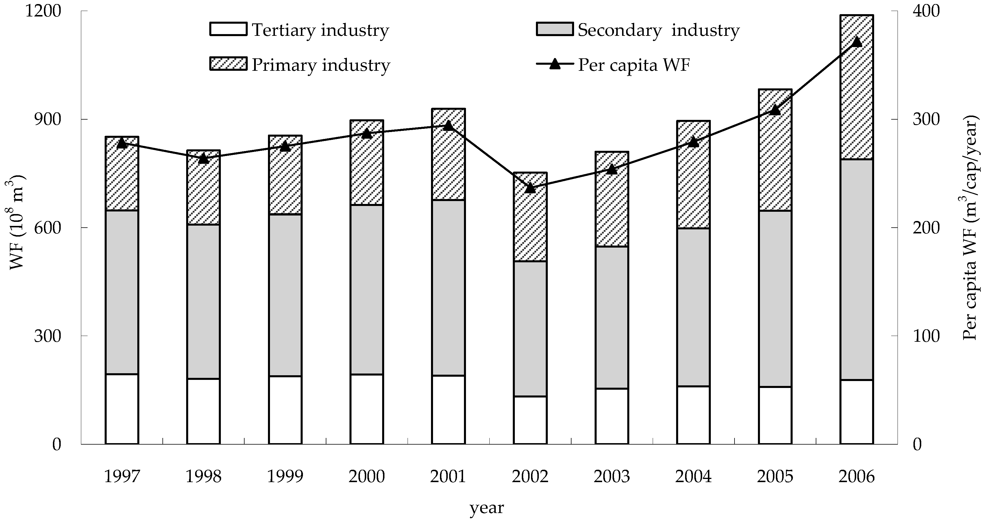
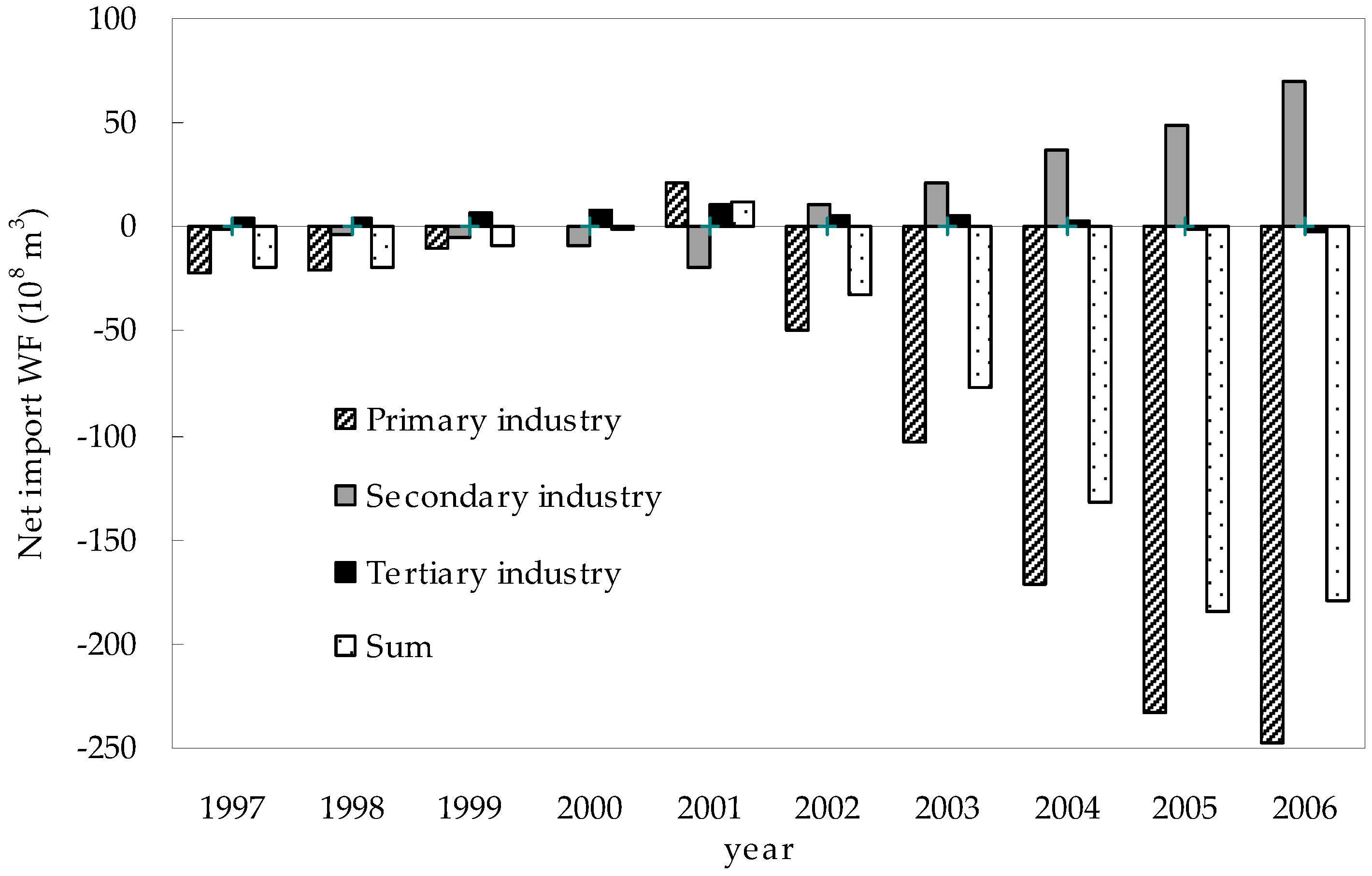
It is found that the 2002 WF decreased to a certain extent (Figure 5). According to China’s grain policy, the export of grain in the Yellow River basin has been increased significantly since 2002. The first industry net external WF is negative in 2002, whose absolute value is more than that of the secondary and tertiary industry, while the total net external water footprint is negative (Figure 6), and the total WF decreased in 2002. However, the secondary industry and tertiary industry are developing rapidly in the regain, total WF during 2002–2006 are showing an increasing trend. According to the meteorological data analysis [51], the precipitation occurs a mutation in crop growth season (April to August), 2002. The precipitation in 2002 is the maximum value during 1997–2006, affecting the agricultural irrigation water. Because the research focuses on the blue WF, so the weather is also the possible reason for the decrease of the calculated WF in 2002.

Water consumption data and our method have disadvantages that need to be improved in future research. First, production sectors use water differently, but the input–output table combines all sectors into three industries and neglects differences. Second, irrigation water was taken to analyse direct agricultural water consumption by IOA, while the efficiency coefficient for irrigation water in the examined watershed ranges from 0.3 to 0.55, so the loss is considerable. A smaller proportion of water withdrawal is actually consumed by the secondary and tertiary industries, and the other flows to nature. Water withdrawn in excess, e.g., due to inefficient irrigation, has not been but should be deducted from the water footprint, which should only include water consumed. Third, domestic water, which yields no economic benefit, is part of the WF. It was neither encompassed in the input–output table nor analysed here.

The RAS method is introduced to investigate variations over time. It extends the input–output table to illustrate changes in human demand for water and reveals changes in the structure of demand for water. It can deduce factors driving demand for water and provide a statistical basis for water resource management. When extending the input–output table, however, we must assume the substitution multiplier is consistent with the production multiplier and that assumption is counter-factual. Moreover, it overly simplifies the RAS method, yielding errors in the extension result. It is necessary to further identify the reliable information and improve the method.

There are various aspects of driving factors of the WF. For instance, it is concluded that it has a large proportion in the secondary industry, but discussion of specific industries is warranted. Conclusions might differ if different indexes were selected. Numerous methods are available for investigating driving factors; those influencing the WF can be analysed by trying other indexes and methods for comparative study.

4.2. Implications

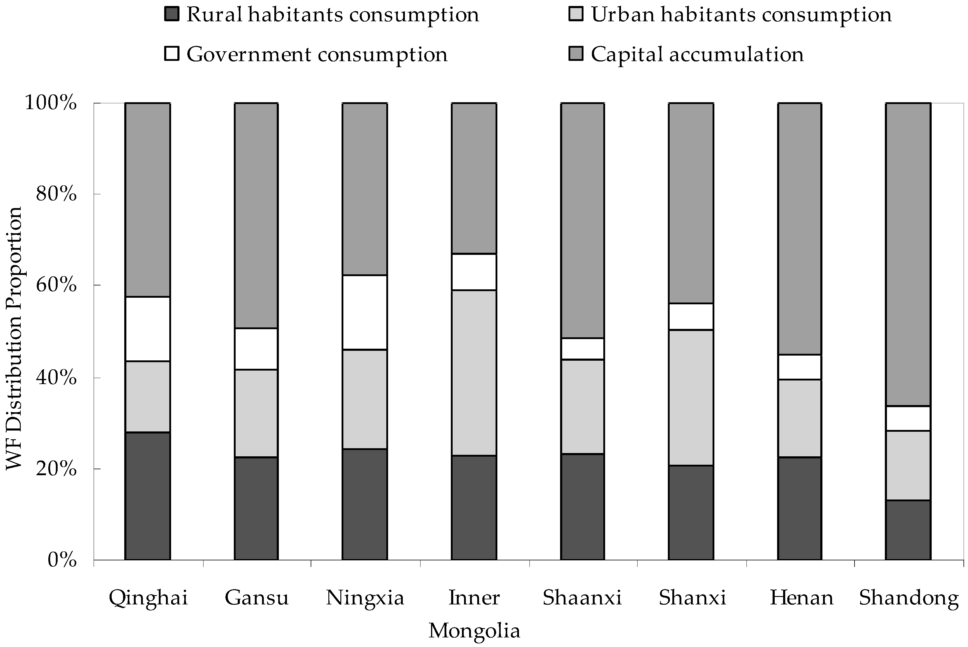
The WF concept seeks to illustrate the hidden links between human consumption and water use [18] and how to reduce the WF by changing human consumption. Some studies have analysed WF by bottom-up and top-down method and have indicated that WF could be decreased by adjusting consumption patterns, especially diet [13]. WF of both consumption and capital accumulation are the main components of total WF, so which can also be reduced by altering capital accumulation structure. However, it is difficult to adjust the two structures.

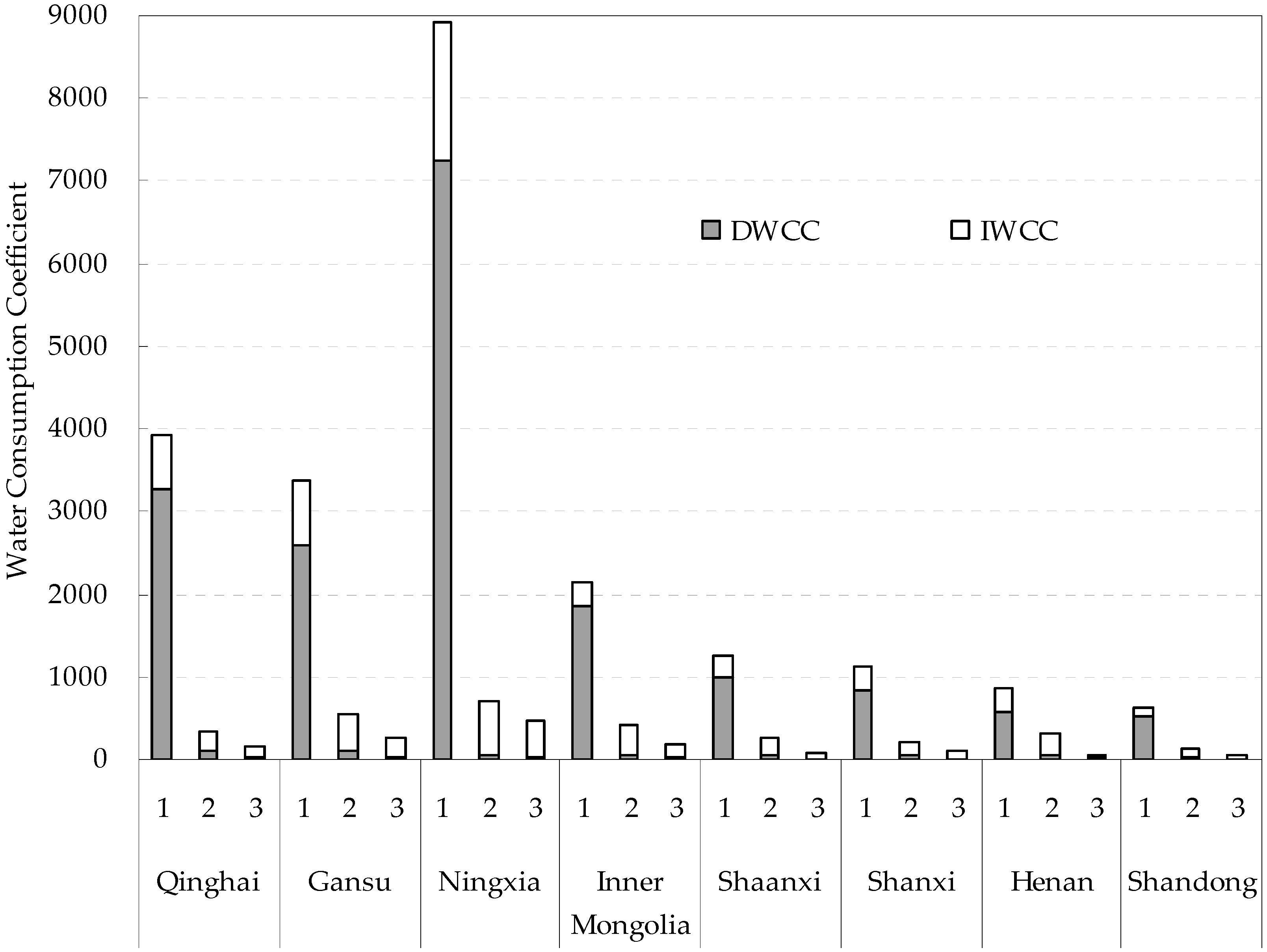
It is more operational to lessen WF by reducing water consumption coefficients and adjusting industrial structures. Agriculture, which accounts for 70% of all water consumption in the basin, plays a main role in the primary industry. Agriculture mainly uses water directly with a low coefficient, especially in the upper reaches, where per capita WF and water consumption coefficients far exceed those in the lower reaches. The study only considered the irrigation water supply when analysed the agricultural water, while a large percent of crops water consumption is the green water which is ignored leading to a great influence on the results.

Upper provinces, such as Qinghai, Gansu, Ningxia and Inner Mongolia, occupy arid areas with scare water resources. The Yellow River is almost the only water source for regions along the river, where sufficient water can be drawn from the river easily and large areas of irrigation have been constructed, notably in Ningxia and Inner Mongolia. In these regions, irrigation is inefficient. For example, irrigation quota of irrigation area in Ningxia and Inner Mongolia is 18,759 m³/hm² and 11,820 m³/hm² respectively, and it is 2708 m³/hm² and 4485 m³/hm² in middle and lower reaches [52]. Crops need more water for dryness, but high agricultural water consumption via flooding irrigation and crops that demand more water (e.g., rice) account for 25% of the seeding area in Ningxia. Thus, it can save much direct water and reduce the water consumption coefficient of the primary industry by heightening agricultural water use efficiency and adjusting plantation structure.

IWCC occupies most of TWCC in the secondary and tertiary industries; the large proportion of IWCC is light industry, catering industry, etc. [29]. These sectors use output of the primary industry as raw materials, with which large amounts of virtual water transfers into the secondary and tertiary industry and whose IWCCs are heightened. Water consumption coefficients in these sectors can be decreased by using fewer products of primary industries that consume more water, for instance, using the lower WF raw materials, or importing the raw materials from the area with high utilization efficiency of water resources through virtual water trade.

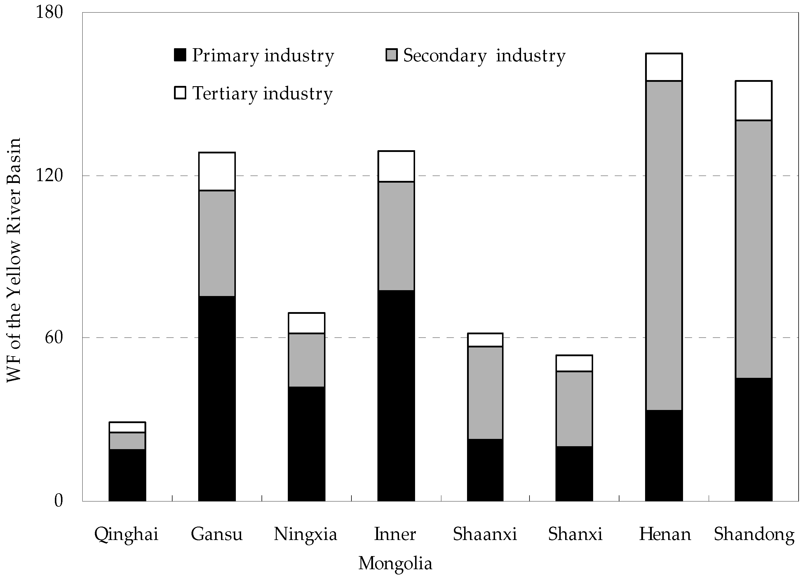
When altering industry structure, according to the lower TWCC of the tertiary industry, the tertiary industry’s share in national economy could be added to reduce the regional water consumption. To alleviate scarcity of water, it is essential to reduce the proportion of the primary industry, but that can be done only if food production is assured in the Yellow River Basin, China’s main grain production area.

In the study, we focus on the dynamic analysis of WF based on the RAS and regression, and just consider the blue WF. For analysing the dynamic of green WF and grey WF, we would have to not only use the above methods, but also combine the process model, remote sensing technology and municipal and environmental data.

5. Conclusions

TWCCs of the three industries in the Yellow River Basin differ greatly and vary significantly among provinces. TWCC of the three industries in Ningxia is far larger than elsewhere. In addition, water consumption coefficients of areas in the river’s upper reaches are generally higher. Tertiary industries and the lower regions of the basin consume water more efficiently.

During the research period, the proportion of net external WF in the total WF of the basin rose from 1.6% initially to 17.9%. The exported virtual water is mainly attributable to agriculture, which constituted more than 40% of water consumption in 2006. The imported virtual water is mainly in the industry, constituting 11.4% of the WF in the secondary industry in 2006. The proportion of final consumption of WF in the total declined constantly in the research period from 54.2% to 41.9% since the consumption rate of the gross national product declined.

In addition, distribution of WF of the final consumption and capital formation in industries differ. The primary industry was dominated by final consumption, whereas the secondary industry was dominated by capital formation. The distribution of total WF in three industries was dominated by the secondary industry, and the proportion of WF of three industries during the research period was relatively stable, with the secondary industry maintaining around 50%.

Apparently, the WF is affected by many socio-economic factors. The proportion of the secondary industry was in the most evident positive correlation with the WF, followed by irrigation area, meat consumption per capita, water consumption per 10,000-yuan increase in added value and population. Obviously, economic scale, population scale and irrigation scale stimulate demand for water. Generally, the unit food output of three industries considerably impacts water resources. However, our analysis indicates that the secondary industry cannot be ignored. The WF of secondary industries along the Yellow River basin is the greatest since mining, metal smelting and power generation take up a huge percentage, followed by textiles, with agricultural products as raw materials indirectly consuming considerable quantities of water. The adjustment of the internal structure of the secondary industry and increase in the proportion of the tertiary industry may restrain growth of the WF. Figures for meat consumption show that consumption by residents along the Yellow River basin will affect demand for water.

In this study, the RAS method is introduced for developing the IOA to study the time variation of WF, and the time series analysis of WF is improved. The method is extended to analyse the WF, which is not only able to explain the change of human’s demand for water resources, but also reveals the change of water resources demand structure from the deep level. Based on the time series of the WF, the driving factors that influence the water resources demand can be deduced, which provide the scientific basis for the management of water resources.

References

1. Hoekstra, A.Y. Sustainable, efficient and equitable water use: The three pillars under wise freshwater allocation. Wiley Interdiscip. Rev. Water 2014, 1, 31–40. [Google Scholar] [CrossRef]
2. Hoekstra, A.Y.; Mekonnen, M.M. The water footprint of humanity. Proc. Natl. Acad. Sci. USA 2012, 109, 3232–3237. [Google Scholar] [CrossRef] [PubMed]
3. Berger, M.; Finkbeiner, M. Water Footprinting: How to address water use in life cycle assessment? Sustainability 2010, 2, 919–944. [Google Scholar] [CrossRef]
4. Hoekstra, A.Y. A critique on the water-scarcity weighted water footprint in LCA. Ecol. Indic. 2016, 66, 564–573. [Google Scholar] [CrossRef]
5. Chapagain, A.K.; Hoekstra, A.Y.; Savenije, H.H.G.; Gautam, R. The water footprint of cotton consumption: An assessment of the impact of worldwide consumption of cotton products on the water resources in the cotton producing countries. Ecol. Econ. 2006, 60, 186–203. [Google Scholar] [CrossRef]
6. Duan, P.; Qin, L.; Wang, Y.; He, H. Spatiotemporal correlations between water footprint and agricultural inputs: A case study of maize production in northeast China. Water 2015, 7, 4026–4040. [Google Scholar] [CrossRef]
7. Guan, D.B.; Hubacek, K. Assessment of regional trade and virtual water flows in China. Ecol. Econ. 2007, 61, 159–170. [Google Scholar] [CrossRef]
8. Hoekstra, A.Y.; Chapagain, A.K.; Aldaya, M.M.; Mekonnen, M.M. The Water Footprint Assessment Manual: Setting the Global Standard; Earthscan: London, UK, 2011. [Google Scholar]
9. Okadera, T.; Okamoto, N. Regional water footprints of the Yangtze River: An interregional input-output approach. Econ. Syst. Res. 2014, 26, 444–462. [Google Scholar] [CrossRef]
10. Zhang, Z.; Yang, H.; Shi, M. Analyses of water footprint of Beijing in an interregional input-output framework. Ecol. Econ. 2011, 70, 2494–2502. [Google Scholar] [CrossRef]
11. Ercin, A.; Hoekstra, A. European water footprint scenarios for 2050. Water 2016, 8. [Google Scholar] [CrossRef]
12. Gheewala, S.H.; Silalertruksa, T.; Nilsalab, P.; Mungkung, R.; Perret, S.; Chaiyawannakarn, N. Water footprint and impact of water consumption for food, feed, fuel Crops production in Thailand. Water 2014, 6, 1698–1718. [Google Scholar] [CrossRef] [Green Version]
13. Hoekstra, A.Y.; Chapagain, A.K. Water footprints of nations: Water use by people as a function of their consumption pattern. Water Resour. Manag. 2007, 21, 35–48. [Google Scholar] [CrossRef]
14. Allan, J.A. Virtual water: A strategic resource. Ground Water 1998, 36, 545–546. [Google Scholar] [CrossRef]
15. Debaere, P. The global economics of water: Is water a source of comparative advantage? Am. Econ. J. Appl. Econ. 2012, 6, 32–48. [Google Scholar] [CrossRef]
16. Zhuo, L.; Mekonnen, M.M.; Hoekstra, A.Y.; Wada, Y. Inter- and intra-annual variation of water footprint of crops and blue water scarcity in the Yellow River basin (1961–2009). Adv. Water Resour. 2016, 87, 29–41. [Google Scholar] [CrossRef]
17. Hoekstra, A.Y.; Chapagain, A.K. Globalization of Water: Sharing the Planet’s Freshwater Resources; Blackwell: Oxford, UK, 2008. [Google Scholar]
18. Hoekstra, A.Y. Human appropriation of natural capital: A comparison of ecological footprint and water footprint analysis. Ecol. Econ. 2009, 68, 1963–1974. [Google Scholar] [CrossRef]
19. Williams, E.D.; Weber, C.L.; Hawkins, T.R. Hybrid framework for managing uncertainty in life cycle inventories. J. Ind. Ecol. 2009, 13, 928–944. [Google Scholar] [CrossRef]
20. Cai, Z.; Shen, L.; Liu, J.; Zhao, X. Applying input-output analysis method for calculation of water footprint and virtual water trade in Gansu Province. Acta Ecol. Sin. 2012, 32, 6481–6488. (In Chinese) [Google Scholar]
21. Leontief, W. Environmental repercussions and the economic structure: An input-output approach. Rev. Econ. Stat. 1970, 52, 262–271. [Google Scholar] [CrossRef]
22. Lenzen, M.; Murray, S.A. A modified ecological footprint and its application to Australia. Ecol. Econ. 2001, 37, 229–255. [Google Scholar] [CrossRef]
23. Ferng, J.J. Local sustainable yield and embodied resources in ecological footprint analysis—A case study on the required paddy field in Taiwan. Ecol. Econ. 2005, 53, 415–430. [Google Scholar] [CrossRef]
24. Singh, S.; Bakshi, B.R. Footprints of carbon and nitrogen: Revisiting the paradigm and exploring their nexus for decision making. Ecol. Indic. 2015, 53, 49–60. [Google Scholar] [CrossRef]
25. Mubako, S.; Lahiri, S.; Lant, C. Input-output analysis of virtual water transfers: Case study of California and Illinois. Ecol. Econ. 2013, 93, 230–238. [Google Scholar] [CrossRef]
26. Feng, K.; Hubacek, K.; Minx, J.; Siu, Y.L.; Chapagain, A.; Yu, Y.; Guan, D.; Barrett, J. Spatially explicit analysis of water footprints in the UK. Water 2011, 3, 47–63. [Google Scholar] [CrossRef]
27. Guan, D.B.; Hubacek, K. A Hydro-Economic accounting and analytical framework for water resources: A case study for North China. J. Environ. Manag. 2008, 88, 1300–1324. [Google Scholar] [CrossRef] [PubMed]
28. Hubacek, K.; Sun, L.X. Economic and societal changes in China and their effects on water use: A scenario analysis. J. Ind. Ecol. 2005, 9, 187–200. [Google Scholar] [CrossRef]
29. Zhao, X.; Chen, B.; Yang, Z.F. National water footprint in an input-output framework—A case study of China 2002. Ecol. Model. 2009, 220, 245–253. [Google Scholar] [CrossRef]
30. Feng, K.; Siu, Y.L.; Guan, D.; Hubacek, K. Assessing regional virtual water flows and water footprints in the Yellow River Basin, China: A consumption based approach. Appl. Geogr. 2011, 32, 691–701. [Google Scholar] [CrossRef]
31. Deng, G.; Ma, Y.; Li, X. Regional water footprint evaluation and trend analysis of China—Based on interregional input-output model. J. Clean. Prod. 2016, 112, 4674–4682. [Google Scholar] [CrossRef]
32. Leontief, W. Quantitative input and output relations in the economic system of the United States. Rev. Econ. Stat. 1936, 18, 105–125. [Google Scholar] [CrossRef]
33. Lahr, M.L.; de Mesnard, L. Biproportional techniques in input-output analysis: Table updating and structural analysis. Econ. Syst. Res. 2004, 16, 115–134. [Google Scholar] [CrossRef]
34. Jalili, A.R. Impacts of aggregation on relative performances of nonsurvey updating techniques and inter temporal stability of input-output coefficients. Econ. Chang. Restruct. 2005, 38, 147–165. [Google Scholar] [CrossRef]
35. Dobrescu, E.; Gaftea, V. On the accuracy of RAS method in an emergent economy. Amfiteatru Econ. J. 2012, 14, 502–521. [Google Scholar]
36. Dobrescu, E. Restatement of the I-O coefficient stability problem. J. Econ. Struct. 2013, 2, 1–67. [Google Scholar] [CrossRef]
37. Yamada, M. Construction of a multi-regional input-output table for Nagoya metropolitan area, Japan. J. Econ. Struct. 2015, 4, 1–18. [Google Scholar] [CrossRef]
38. Liu, J.G.; Williams, J.R.; Zehnder, A.J.B.; Yang, H. GEPIC—Modelling wheat yield and crop water productivity with high resolution on a global scale. Agric. Syst. 2007, 94, 478–493. [Google Scholar] [CrossRef]
39. National Economy Accounting Department of National Bureau of Statistics. Regional Input–Output Tables of China 2002; Chinese Statistics Press: Beijing, China, 2008.
40. Yellow River Conservancy Commission. Bulletin of Yellow River Water Resources; Yellow River Water Resources Press: Zhengzhou, China, 2007. [Google Scholar]
41. Zhang, Q.; Peng, J.; Singh, V.P.; Li, J.; Chen, Y.D. Spatio-temporal variations of precipitation in arid and semiarid regions of China: The Yellow River basin as a case study. Glob. Planet. Chang. 2014, 114, 38–49. [Google Scholar] [CrossRef]
42. Stone, J.M. Input-Output Relationships 1954–1966; MIT Press: Cambridge, MA, USA, 1963. [Google Scholar]
43. Härdle, W.; Simar, L. Applied Multivariate Statistical Analysis; Springer: Berlin, Germany, 2003. [Google Scholar]
44. Draper, R.N.; Smith, H. Applied Regression Analysis; Wiley: New York, NY, USA, 1998. [Google Scholar]
45. Siddik, K.; Irfan, D.; Askin, K. Factor Analysis Scores in a Multiple Linear Regression Model for the Prediction of Carcass Weight in Akkeci Kids. J. Appl. Anim. Res. 2007, 31, 201–204. [Google Scholar]
46. Thayer, J.D. Interpretation of Standardized Regression Coefficients in Multiple Regression. In Proceedings of the Annual Meeting of the American Educational Research Association, Chicago, IL, USA, 3–7 April 1991.
47. Zhuo, L.; Mekonnen, M.M.; Hoekstra, A.Y. Sensitivity and uncertainty in crop water footprint accounting: A case study for the Yellow River basin. Hydrol. Earth Syst. Sci. 2014, 18, 2219–2234. [Google Scholar] [CrossRef]
48. Dong, H.; Geng, Y.; Fujita, T.; Fujii, M.; Hao, D.; Yu, X. Uncovering regional disparity of China’s water footprint and inter-provincial virtual water flows. Sci. Total Environ. 2014, 500–501, 120–130. [Google Scholar] [CrossRef] [PubMed]
49. International Organization for Standardization (ISO). ISO 14046: Environmental Management–Water Footprint–Principles, Requirements and Guidelines; International Organization for Standardization: Geneva, Switzerland, 2014. [Google Scholar]
50. Boulay, A.M.; Hoekstra, A.Y.; Vionnet, S. Complementarities of water-focused life cycle assessment and water footprint assessment. Environ. Sci. Technol. 2013, 47, 11926–11927. [Google Scholar] [CrossRef] [PubMed]
51. He, J.P.; He, Z. Spatio-temporal characteristics of extreme precipitation event in Yellow River basin in recent 53 years. Ecol. Environ. Sci. 2014, 23, 95–100. [Google Scholar]
52. Jia, S.; Zhang, S.; Wang, H. Reasons of high irrigation quota and potential of water-saving in Ning-Meng Irrigation Area. Resour. Sci. 2003, 25, 29–34. [Google Scholar]
Figure 1. The studied nine provinces (municipalities) in the Yellow River Basin.
Water 08 00363 g001
Figure 2. Water consumption coefficients of the Yellow River Basin (m3/104 Yuan). Note: 1, 2 and 3 in abscissa stand for the primary, secondary and tertiary industries, respectively.
Water 08 00363 g002
Figure 3. Water footprint (WF) distribution proportion of the Yellow River Basin (m3/104 Yuan). Note: 1, 2 and 3 in abscissa stand for the primary, secondary and tertiary industries, respectively.
Water 08 00363 g003
Figure 4. Water footprint (WF) of the Yellow River Basin in 2002 (billion m3).
Water 08 00363 g004
Figure 5. Variation of total WF and per capita WF of consumption in the Yellow River basin from 1997 to 2006.
Water 08 00363 g005
Figure 6. Variation of the net import water footprint (WF) of the Yellow River basin from 1997 to 2006.
Water 08 00363 g006
Figure 7. Comparison between the actual value and the predicted value of WF based on the linear regression.
Water 08 00363 g007