Addressing Groundwater Declines with Precision Agriculture: An Economic Comparison of Monitoring Methods for Variable-Rate Irrigation

Abstract

Irrigated row-crop agriculture is contributing to declining groundwater in areas such as the Mississippi Delta region of eastern Arkansas. There is a need to move toward sustainable levels of groundwater withdrawal. Recent improvements in remote monitoring technologies such as wireless soil moisture sensors and unmanned aerial vehicles offer the potential for farmers to effectively practice site-specific variable-rate irrigation management for the purpose of applying water more efficiently, reducing pumping costs, and retaining groundwater. Soil moisture sensors and unmanned aerial vehicles are compared here in terms of their net returns per acre-foot and cost-effectiveness of aquifer retention. Soil moisture sensors ($9.09 per acre-foot) offer slightly more net returns to producers than unmanned aerial vehicles ($7.69 per acre-foot), though costs associated with unmanned aerial vehicles continue to drop as more manufacturers enter the market and regulations become clear.

1. Introduction

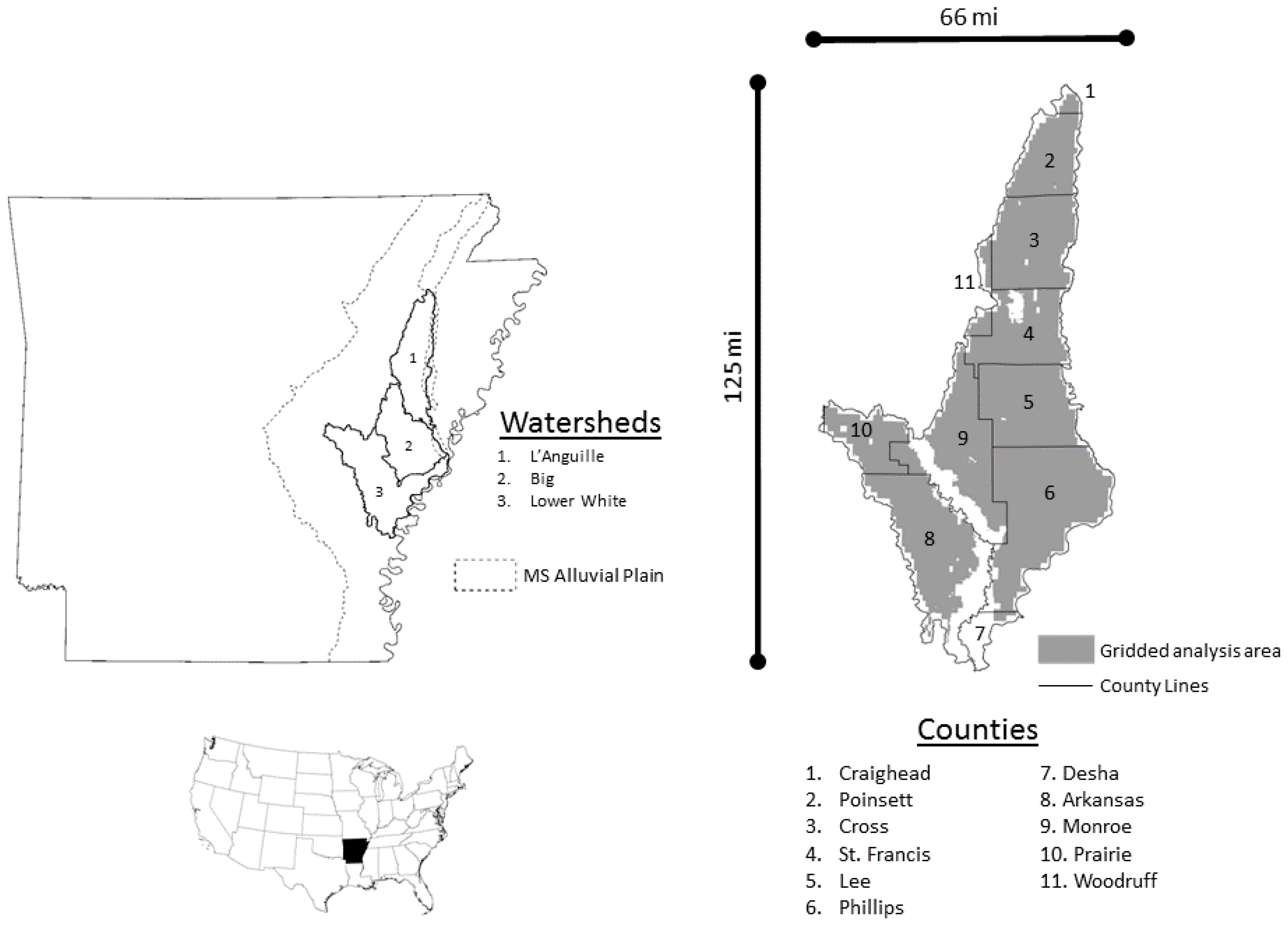
More than 80 percent of the consumptive water use in the United States, which is the water lost to the environment, goes to irrigated agriculture [1]. The Mississippi River Valley alluvial aquifer of the Delta is used by agriculture in Arkansas, Missouri, Mississippi, and Louisiana, and irrigated acreage has more than doubled from 1982 to 2007 [1]. Critical groundwater areas in the Delta region of eastern Arkansas continue to experience decline as groundwater demand outpaces recharge. Demand for groundwater constitutes 81% of the total water demand in the East Arkansas Region (Figure 1), and a groundwater gap of over seven million acre-feet is projected for 2050 [2]. A declining aquifer raises the cost of pumping groundwater and risks the future profitability of agriculture, the dominant industry in the region. These risks are amplified by prospects of long-term drought and climate uncertainty. Additional benefits to society of a greater aquifer volume include the avoidance of subsidence, less seepage of surface water from riparian areas vital to wildlife, and less pumping of underlying aquifers used for drinking water in towns. There is a need to move toward sustainable levels of groundwater withdrawal.

Precision agriculture provides the potential to enhance irrigation efficiency through site-specific variable-rate irrigation management of crops. Irrigation efficiency is defined as the ratio of applied water that is beneficially used for crop growth to the total amount of applied water [3]. The irrecoverable fraction of applied water includes runoff from a geographic area, evaporation, and plant evapotranspiration [3,4]. Some fraction of applied irrigation water is recoverable, re-entering the aquifer in the future as deep percolation [3,4]. Field-level spatial variability in soil characteristics results in spatial variability of irrigation efficiency and can lead to over- or under- application of water under uniform application conditions. In most cases, a farmer will tend to over-apply to account for uneven distribution of water in the field and maximize yield [5]. Mapping the variability of appropriate field conditions using remote monitoring methods can allow a farmer to apply variable-rate irrigation management and maintain yields while decreasing water use and groundwater pumping [6,7,8,9].

Precision agriculture adoption is one means by which farmers can limit the over-application of crop production inputs such as irrigation water and nutrients by using technology to inform site-specific management according to spatially localized conditions [8,10,11]. The spatial information technologies that have enabled precision agriculture include global positioning systems, geographic information systems, remote sensing, and variable-rate application technologies [12]. Precision agriculture involves combining the functions of these technologies to help with decision-making about crop and soil management in specific field locations [13].

For the purposes of managing variable irrigation rates, two different paradigms of monitoring field-level spatial variability have emerged and proved effective: one based on monitoring soil properties and the other on monitoring plant conditions [6,14,15]. Hedley and Yule [6] demonstrated the potential to reduce irrigation water use by using soil–water balance to inform variable-rate irrigation of pre-mapped management zones at two sites in New Zealand. Stone et al. [16] demonstrated the potential of similar methods in the humid Eastern U.S. Soil-based methods are thought to be superior because they more directly measure water-related stress as a function of plant available water content, whereas it can be more difficult with plant-based methods to separate the effect of the soil moisture property from that of other possible stresses such as nutrient deficiency [17,18]. Soil water measurements using soil moisture sensors, however, are only accurate for a small area, and soil water content is highly variable spatially and temporally [19]. There is evidence that relative spatial variability of soil water content is persistent over time, further indicating the feasibility of variable-rate irrigation based on management zones [20,21].

Networks of remote soil moisture sensors have shown the ability to effectively inform variable-rate irrigation and contribute to improvements in irrigation efficiency [6,8,11,15,18]. Though the soil moisture sensors themselves perform in-situ measurement of soil properties, these networks of sensors are monitored wirelessly by either an automated system or a user physically removed from the measurement site. In the past, installation of enough soil moisture sensors to capture soil variability has proven costly for farmers and has limited technology adoption [22,23]. This technology is getting better and more affordable at the same time that unmanned aerial vehicles are also becoming more economical for the purposes of plant-based remote sensing. Unmanned aircraft can deliver a variety of sensing devices including visual, multispectral, and thermal to monitor different aspects of plant health. There is even potential in the future for these vehicles to serve as the medium by which important production inputs such as seed, fertilizer, and chemical are applied [24]. Though unmanned aerial vehicles have not been commonly used in agriculture to this point, the Department of Transit and Federal Aviation Administration have recently enacted a clear regulatory framework for small unmanned aerial aircraft, and many expect this to spur more widespread adoption in commercial uses such as agriculture [25,26].

We compare the two remote monitoring methods, soil moisture sensors and unmanned aerial vehicles, for cost-effectiveness and net return per acre-foot of aquifer retention by modeling crop production and groundwater use across a spatially-explicit farm landscape in the Delta region of eastern Arkansas. The model evaluates the optimal crop mix and irrigation practices to maximize farm returns across the gridded farm landscape. Spatial variation in crop yields, aquifer thickness, and the costs of groundwater pumping all influence the spatial-dynamic path of optimal management [27]. The effectiveness of the remote monitoring methods for enhancing profitability and decreased pumping depends on these spatial variations.

The area for the application of our model encompasses three eight-digit hydrologic unit code (HUC) watersheds overlying the Mississippi River Valley alluvial aquifer where groundwater levels are critical (Figure 1). Eight-digit HUCs define the drainage area of a sub-basin of a river [28]. In addition to remote monitoring and variable-rate irrigation, we allow for the construction of on-farm reservoirs and tail-water recovery systems to help reduce pumping costs and promote recharge of the underlying aquifer. The impacts of remote monitoring and variable-rate irrigation are evaluated with and without the presence of reservoirs on the landscape. There are also ranges of potential costs and irrigation efficiencies associated with these remote monitoring methods, and the implications of these for investment in the technologies is considered. In addition, the effectiveness of policies that encourage the adoption of the remote monitoring for improved water management and aquifer retention is compared to typical fee and quantity policies for conservation. We describe the model for the dynamics of land cover, water use, and profit maximization in Section 2. Data for crop land and model parameters are presented in Section 3. Section 4 discusses results and sensitivity analyses. We conclude with a discussion of major findings and future research needs.

2. Materials and Methods

2.1. Methods

We consider how crop patterns and irrigation use change as a farm collective maximizes profits on the landscape over time. The model is then used to evaluate which approach to precision irrigation is more cost-effective for reducing groundwater pumping or delivers higher net return per acre-foot of aquifer retention.

2.1.1. Land Cover

The land cover of the farm landscape includes crops, reservoirs, and conserved land set aside through a rental program of the government. The chosen crops generate economic returns, and irrigation depletes groundwater. The landscape is spatially heterogeneous due to differences in long-term investment in farm practices, soil types, and access to water resources [29,30,31]. A time horizon T is chosen for a single generation of farmers to observe how depletion of the aquifer influences production decision, and a grid of m cells (sites) represents spatial differences.

Major crops on the landscape include rice, irrigated soybean, corn, and cotton, non-irrigated sorghum and soybean, and double-cropped irrigated soybean with winter wheat. The model tracks acreage across n number of land cover types j, including each of the crops, reservoirs that have tail-water recovery, and the U.S. Department of Agriculture’s Conservation Reserve Program (CRP). L_ijt denotes the amount of land (acres) at site i in land cover type j at the end of period t. At the end of each period t, which is a 10-year interval, we assume any other land cover j can become on-farm reservoirs and tail-water recovery or CRP. A 10-year interval is appropriate because we expect crop rotations to emphasize more profitable crops over a decade, and this is a typical contract period for CRP land. A profit-maximizing farmer may switch land out of irrigated crops into non-irrigated crops with declining groundwater availability at the end of each period.

The initial land availability equals the sum of the land covers chosen for site i at any time t (Equation (1)).

$${\displaystyle {\sum }_j^n{L}_{ijt}}={\displaystyle {\sum }_j^n{L}_{ij0}},\mathrm{for}j=\mathrm{crops},\mathrm{CRP},\text{ on-farm reservoirs}$$

(1)

2.1.2. Irrigation

The average annual irrigation that crop j receives to supplement precipitation, wd_j, is the demand for irrigation in acre-feet. The groundwater stored in the aquifer beneath site i at the end of the period t is AQ_it. The water that comes from the on-farm reservoirs is RW_it, and the water from well pumping is GW_it. There is recharge of the groundwater, nr_i, that occurs naturally from precipitation, streams, and underlying aquifers each period.

Equation (2) shows the acre-feet of water stored in an acre reservoir as

$$\left({\omega }_{\max }+{\omega }_{\min }\right)-\frac{{\omega }_{\max }}{{\displaystyle {\sum }_j^n{L}_{ij0}}}{L}_{iRt},$$

(2)

which includes $L_{iRt}$ as the acres in reservoirs at time t, and the total acreage at site i, ${\displaystyle {\sum }_j^n{L}_{ij0}}$. If the reservoir occupies the entire site i and only the rainfall fills the reservoir, then the low-end acre-feet of water that fills each acre of reservoir is ${\omega }_{\min }$. If the reservoir is small compared to the entire site, then $\frac{{\omega }_{\max }}{{\displaystyle {\sum }_j^n{L}_{ij0}}}{L}_{iRt}$ is close to zero, and the recovery of the runoff and rainfall fills the reservoir to near capacity in acre-feet per reservoir acre of $\left({\omega }_{\max }+{\omega }_{\min }\right)$. This does not account for temporal variability in the evaporation, leakage, and the timing of rainfall within each period, which could influence the values of ${\omega }_{\max }$ and ${\omega }_{\min }$ for the reservoir.

The intensity of well pumping across the landscape influences aquifer depletion variability over space. The proportion of the underground flow into the aquifer at site k and out of site i when an acre-foot is pumped from a well at site k is p_ik, which depends on the distance and the lateral speed of underground water movement based on the soil profiles observed between sites [27]. This means the groundwater that leaves site i is ${\displaystyle {\sum }_k^m{p}_{ik}G{W}_{kt}}$. We assume pumps have the same efficiency and power units to deliver a fixed amount of water per minute.

The water used for irrigation must be less than the water available from reservoirs and wells (Equation (3)), and Equation (4) indicates the water stored in the reservoirs must be greater than the water used from the reservoirs. The aquifer volume in the previous period less the spatially weighted proportion of water pumped from the surrounding sites plus natural recharge equals the current aquifer volume (Equation (5)). The cost of pumping groundwater at a site, GC_it, depends on the cost to lift an acre-foot of water by one foot, c^p, and the initial depth to the groundwater, dp_i. The depletion of the aquifer volume, $\left(A{Q}_{i0}-A{Q}_{it}\right)$, divided by the area of the site, ${\displaystyle {\sum }_j^n{L}_{ij0}}$, shows how much the depth to the aquifer increases. Capital costs per acre-foot for the well, which accounts for new well drilling in response to aquifer decline, is c^c (Equation (6)).

$${\displaystyle {\sum }_{j=1}^{n}w{d}_j{L}_{ijt}}\le G{W}_{it}+R{W}_{it}$$

(3)

$$R{W}_{it}\le \left(\left({\omega }_{\max }+{\omega }_{\min }\right)-\frac{{\omega }_{\max }}{{\displaystyle {\sum }_j^n{L}_{ij0}}}{L}_{iRt}\right)L_{iRt}$$

(4)

$$A{Q}_{it}=A{Q}_{i(t-1)}-{\displaystyle {\sum }_k^m{p}_{ik}G{W}_{kt}}+n{r}_i$$

(5)

$$G{C}_{it}=c^c+c^p\left(d{p}_i+\frac{\left(A{Q}_{i0}-A{Q}_{it}\right)}{{\displaystyle {\sum }_j^n{L}_{ij0}}}\right)$$

(6)

2.1.3. Profit Objective

The cost to produce an acre of the crop, excluding the irrigation costs ca_j and the price per conventional unit of the crop, is pr_j and constant in real terms. We assume no productivity growth trend for the constant yield of crop j per acre at site i, y_ij. Excluding the costs of irrigation, the net value for crop j is then pr_jy_ij − ca_j per acre. The CRP payment per acre to the landowner, pr_crpy_icrp, with yield normalized to one and price is the payment per acre, less the cost to establish and maintain an acre of CRP (ca_crp) is the net value per acre of CRP. The reservoir pumping cost per acre-foot is c^rw, and the per acre capital and maintenance cost of a reservoir each period is c^r. We make values over time comparable in monetary terms using the real discount factor, ${\delta }_t$.

Equation (7) indicates the economic objective to maximize the present value of farm profits over the fixed horizon T by changing the amount of land in each crop or CRP, the reservoir water use, and groundwater use, namely L_ijt, RW_it, and GW_it. The fixed horizon T is a 30 years in length, and each period is ten years in length. The non-negativity constraints on land, water use, and the aquifer are shown in Equation (8).

$$\underset{L_{ijt},R{W}_{it},G{W}_{it}}{\max }:{\displaystyle \sum _{t=1}^T{\delta }_t\left({\displaystyle \sum _{i=1}^m{\displaystyle \sum _{j=1}^n\left(p{r}_j{y}_{ij}-c{a}_j\right)L_{ijt}-c^r{L}_{iRt}-c^{rw}R{W}_{it}-G{C}_{it}G{W}_{it}}}\right)}$$

(7)

subject to:

$$L_{ijt}\ge 0,R{W}_{it}\ge 0,G{W}_{it}\ge 0,A{Q}_{it}\ge 0$$

(8)

and the spatial dynamics of land and irrigation (Equations (1)–(6)). We use the non-linear programming solver CONOPT from AKRI Consulting and Development to perform the optimization in the Generalized Algebraic Modeling System [32].

2.1.4. Cost-Effectiveness and Net Returns per Acre-Foot of Aquifer Retention with Precision Irrigation

The cost-effectiveness of aquifer retention using precision irrigation is calculated by first finding the difference in the present value of costs and the difference in the final aquifer volume between the baseline and a model with only the soil moisture sensors or only the unmanned aerial vehicles. The baseline model supposes no adoption of soil moisture sensors or unmanned aerial vehicles, and this is compared to models with only soil moisture sensors or only unmanned aerial vehicles. The division of the difference in the present value of costs by the difference in the final aquifer volume indicates the cost effectiveness of a particular precision irrigation technique. The net returns per acre-foot of aquifer retention come from the division of the difference in the present value of net returns by the difference in the final aquifer volume.

2.1.5. Sensitivity Analyses and Conservation Policies

The baseline, soil moisture sensors only, and unmanned aerial vehicle only models are then run again with on-farm reservoirs on the landscape to see how this changes crop choice, cost-effectiveness, and net-benefit assessments. Another sensitivity analysis considers low- and high-range costs and water-use efficiencies for each of the crops using either the soil moisture sensors or the unmanned aerial vehicles.

Policy options for groundwater conservation include cost-share for the precision irrigation techniques of soil moisture sensors and unmanned aerial vehicles by modifying ca_jk. Scenarios regulating groundwater pumping levels and taxing groundwater pumping cost GC are also compared. The cost share is 60% for soil moisture sensors and unmanned aerial vehicles based on the rates from similar improvements under the Natural Resource Conservation Service’s (NRCS) Agricultural Water Enhancement Program [33]. We chose a regulation on groundwater pumping to 220% of initial levels and a fee on groundwater pumping costs of 4% to achieve groundwater conservation similar to the cost share on reservoir construction. Farm net returns in policy scenarios include the payments to or receipts from the government because of the policy. Groundwater conservation cost is calculated as the policy cost (baseline farm net returns less the farm net returns plus government revenue) divided by the change in aquifer level between the policy option and the baseline. All policy scenarios allow for construction of on-farm reservoirs.

2.2. Data

The outer boundary of the study area consists of three eight-digit HUC watersheds in the Arkansas Delta region with critical groundwater areas and non-point source pollution priorities (Figure 1). These watersheds overlap eleven Arkansas counties, and the average for the past 5 years of crop yields by county is a proxy for the yield of the crops [29]. We evaluate crop mix and irrigation methods on a landscape with spatial heterogeneity by dividing the study area into 2724 sites of approximately 600 acres each. At this size, sites approximate farm scale and realistically capture the dynamics of the aquifer in response to pumping across the landscape. Sites having entirely non-cropland uses in the 2013 Cropland Data Layer (CDL), e.g., public lands, water, and urban areas, are removed [34]. The initial acreage of rice, corn, cotton, soybeans, and sorghum comes from the 2013 CDL, and on the basis of harvested acreage for 2010–2011 the soybean acreage is split into non-irrigated soybean, irrigated soybean, and double crop soybeans (

Table 1. Descriptive statistics of the model data across the sites of the study area.

Variable	Definition	Mean	Std. Dev.	Sum (Thousands)
Li,rice	Initial acres of rice	81	99	221
Li,corn	Initial acres of corn	52	77	143
Li,cotton	Initial acres of cotton	10	40	26
Li,isoy	Initial acres of irrigated soybean	165	97	449
Li,dsoy	Initial acres of dry land soybean	57	49	155
Li,dsorg	Initial acres of dry land sorghum	7	23	20
Li,dbl	Initial acres of double crop irrigated soybean and winter wheat	47	73	129
yi,rice	Annual rice yield (cwt per acre) 1	71	3	-
yi,cotton	Annual cotton yield (pounds per acre) 1	1012	148	-
yi,corn	Annual corn yield (bushels per acre) 1	166	11	-
yi,isoy	Annual irrigated soybean yield (bushels per acre) 1	42	4	-
yi,dsoy	Annual dry land soybean yield (bushels per acre) 1	25	3	-
yi,dsorg	Annual dry land sorghum yield (bushels per acre) 1	69	12	-
yi,dbl	Annual double crop irrigated soybean yield (bushels per acre) 1	34	1	-
yi,wheat	Annual winter wheat yields (bushels per acre) 1	57	5	-
dpi	Depth to water (feet)	57	31	-
AQi	Initial volume of the aquifer (acre-feet)	28,047	11,972	76,398
K	Hydraulic conductivity (feet per day)	226	92	-
nri	Annual natural recharge of the aquifer per acre (acre-feet)	0.45	0.19	1.22

Notes: Number of sites is 2724; ¹ The mean and the standard deviation of the county yields come from the 11 counties of the study area.

) [35]. In addition, to account for the time-value of money in the optimization of returns over the 30-year period, the yield of the 30-year Treasury Bond over the last decade suggests and we employ a real discount rate of 5% [36]. Over the last 5 to 10 years the real discount rate is close to 2%, but looking back over 30 years a 5% discount rate is a better approximation.

2.2.1. Aquifer

Table 1 shows the initial depth to the water table and volume of the Alluvial aquifer from the Arkansas Natural Resources Commission [31]. The acreage of the site times the saturated thickness of the aquifer is the volume of the aquifer at site i. The natural recharge, nr_i, of the Alluvial aquifer is based on a calibrated model of recharge for the period 1994 to 1998 associated with precipitation, flow to or from streams, and other groundwater fluxes [37]. It is important to note that improvements in irrigation efficiency resulting from the use of precision irrigation impact both recoverable and irrecoverable fractions of applied irrigation water. Some improvement comes in the form of decreased amounts of direct evaporation and runoff which directly contributes to groundwater conservation [4,38,39]. This is accompanied, however, by decreased amounts of the recoverable fraction of deep percolation. The proportions of improved irrigation efficiency attributable to recoverable and irrecoverable fractions are not precisely known. Furthermore, decision makers in many aquifer systems consider losses to deep percolation to be irrecoverable fractions due to the amount of time it takes for water to reach a reusable state [3,40,41]. With these facts in mind, we do not consider differences in the rate of recoverable deep percolation resulting from precision irrigation in our modeled calculations of aquifer levels.

The spatial weight (p_ik) is the expected proportion of groundwater that flows underground out of site i into site k when an acre-foot of groundwater is pumped from site k, where p_ik is based on the distance between sites i and k, the saturated thickness, and hydraulic conductivity of the aquifer [27]. These dynamics dictate how well pumping reduces the aquifer beneath the surrounding cells. The aquifer below the well and the aquifer of the surrounding sites declines in response to well pumping. Water flows from the aquifer of surrounding sites into the site with the cone of depression created by the pumped well. The distance from the pumped site and the hydraulic conductivity of the aquifer, as described above, influence the volume of the underground flow from the surrounding sites. Clark, Westerman and Fugitt [30] use spatially coarse pilot points to digitize the hydraulic conductivity of the aquifer measured by feet per day. The spatial weight depends on the volume of underground flow, and this determines how much an acre-foot of water pumped from a well reduces the aquifer beneath the surrounding sites.

2.2.2. Farm Production and the On-Farm Reservoir and Tail-Water Recovery System

The costs of production by crop from the 2014 Crop Cost of Production estimates, excluding irrigation, are shown in

Table 2. Value of economic and irrigation model parameters.

Parameter	Definition	Value
prrice	Price of rice ($/cwt)	14.00
prcot	Price of cotton ($/lbs)	0.88
prcorn	Price of corn ($/bushel)	5.50
prsoy	Price of soybeans ($/bushel)	11.99
prsorg	Price of sorghum ($/bushel)	5.23
prwht	Price of wheat ($/bushel)	6.39
carice	Annual production cost of rice ($/acre)	646
cacorn	Annual production cost of corn ($/acre)	632
cacotton	Annual production cost of cotton ($/acre)	742
caisoy	Annual production cost of irrigated soybean ($/acre)	349
cadsoy	Annual production cost of dry land soybean ($/acre)	289
cadsorg	Annual production cost of dry land sorghum ($/acre)	270
cadbl	Annual production cost of double crop irrigated soybean and winter wheat ($/acre)	656
wdrice	Annual irrigation per acre of rice (acre-feet)	2.5
wdcorn	Annual irrigation per acre of corn (acre-feet)	1.0
wdcotton	Annual irrigation per acre of cotton (acre-feet)	1.0
wdisoy	Annual irrigation per acre of full-season soybean (acre-feet)	1.0
wddbl	Annual irrigation per acre of double crop soybean (acre-feet)	0.75
ωmin	Low-end annual capacity per acre of reservoir (acre-feet)	4.0
ωbase	Baseline annual capacity per acre of reservoir (acre-feet)	7.5
ωmax	High-end annual capacity per acre of reservoir (acre-feet)	11.0
c′min	Low-end annual per acre cost of reservoir ($/acre) a	285
c′base	Baseline annual per acre cost of reservoir ($/acre) a	377
c′max	High-end annual per acre cost of reservoir ($/acre) a	777
$c^{rw}$	Cost to re-lift an acre-foot to and from the reservoir ($/acre-foot)	22.62
cp	Cost to raise an acre-foot of water by one foot ($/foot)	0.55
${\delta }_t$	Discount factor	0.98

Notes: ^a this is the annual amortized construction cost and maintenance cost for each acre of reservoir.

[42]. The crop specific irrigation water use comes from the Division of Agriculture [29]. The 5-year average of December futures prices for harvest time contracts for all crops are used for the crop prices [43]. The sign-ups in Arkansas as of March 2015 indicate the CRP payment per acre [44].

Variable irrigation costs from wells or reservoirs include fuel, lube and oil, irrigation labor, and poly pipe for furrow irrigation plus the levee gates for the flood irrigation of rice [45]. The fuel cost per acre-foot of groundwater depends on the fuel needed to raise water from the aquifer, which depends on the depth to the aquifer and the efficiency of the pump, gear-head, and motor. The groundwater pump is assumed to deliver 1800 gallons per minute and the stationary re-lift pump for the reservoir and tail-water recovery system to deliver 2000 gallons per minute [45]. The range in diesel use for a well is 13 gallons of diesel per acre foot for a 100 foot well to 26 gallons of diesel per acre foot for a 200 foot well, and 6 gallons of diesel is needed per acre-foot for pumping water to and from the reservoir [29]. To account for the oil and lube for irrigation equipment, we add 10% to the fuel cost of $3.77 per gallon of diesel fuel [46]. To calculate a capital cost per acre-foot pumped, the capital cost of the irrigation equipment is amortized, and this is divided by the acre-feet pumped from the well [45]. These technologies and costs characterize the conventional irrigation methods of our baseline scenario.

On-farm reservoir/tail-water recovery construction and maintenance costs for various reservoir sizes were estimated using Modified Arkansas Off-Stream Reservoir Analysis (MARORA) to obtain capital cost estimates [47]. Since a majority of the construction cost for a reservoir rests on the cost to move one cubic yard of soil, this cost was updated from $1 per cubic yard to $1.2 per cubic yard to reflect changes in fuel cost. The remainder of the investment and maintenance cost comes from MARORA estimates and includes re-lift pumps for moving water from the tail-water pit to the reservoir and from the reservoir to the field. The reservoir and tail-water recovery system capital cost is amortized to annual per acre payments. The minimum volume of water (ω_min) an acre reservoir will hold comes from the tail-water recovery system collecting rainfall alone to fill a reservoir by 1.4 acre-feet of water [48]. The maximum capacity accounting for evaporation of 11 acre-feet per acre is based on irrigation runoff supplementing the rainfall runoff [47].

2.2.3. Production Cost and Water Use Factors for Remote Monitoring Technologies

Model scenarios involving precision irrigation technologies require adjustment factors for production cost and water use.

Table 3. Value of production cost and irrigation efficiency factors.

Adjustment Factor	Scenario	Rice	Corn	Cotton	Irrigated Soybean	Double Crop Soybean
Baseline
Production cost ($/acre)		646	632	742	349	656
Water use (acre-feet)		2.5	1	1	1	0.75
Soil Moisture sensors
Production cost factor a	Low e	1.015	1.016	1.013	1.028	1.015
	Base	1.023	1.024	1.020	1.043	1.023
	High e	1.041	1.042	1.035	1.075	1.040
Irrigation efficiency factor b	Low f	0.64	0.64	0.64	0.64	0.64
	Base	0.88	0.88	0.88	0.88	0.88
	High f	0.92	0.92	0.92	0.92	0.92
Unmanned aerial vehicles
Production cost factor c	Low e	1.014	1.014	1.012	1.025	1.013
	Base	1.022	1.022	1.019	1.040	1.021
	High e	1.039	1.040	1.034	1.073	1.039
Irrigation efficiency factor d	Low f	0.69	0.69	0.69	0.69	0.69
	Base	0.93	0.93	0.93	0.93	0.93
	High f	0.98	0.98	0.98	0.98	0.98

Notes: ^a [52,53,54]; ^b [15]; ^c [52,55]; ^d [14]; ^e [63,64]; ^f [49].

reports these factors by crop type. In addition to a baseline scenario, adjustment factors are provided for sensitivity analyses involving low and high cost and water use scenarios. Water use improvements resulting from soil moisture sensor-informed variable-rate irrigation were taken from LaRue [15], who conducted field experiments to determine the benefits of variable-rate irrigation relative to applying uniform irrigation amounts. Hedley et al. [7] and Hedley, Yule, and Bradbury [9] also observed comparable water savings over several years using similar methods. The adjustment factor for water use in the baseline scenario draws from these experimental results, while the high and low adjustment factors used for sensitivity analysis come from discussion in Hedley et al. [49]. The soil moisture sensor network and variable-rate system used in the field experiments were similar to Vories et al. [50], and costs associated with these methods were gathered from several sources and used to calculate additional per-acre production costs associated with the soil moisture sensors. Production cost adjustment factors were calculated separately for each of the crop types. Soil mapping is necessary for delineating management zones, and services are available for approximately $4.00 per acre [51,52,53,54]. An interval of five years is used for the re-delineation of management zones. The network of soil moisture sensors costs approximately $8400 for a farm similar in size to a single grid cell (600 acres) in our modeled study area, while a digital data logger costs approximately $1300, and both may need replacing approximately every five years [55]. Costs for a retrofitted variable-rate irrigation system approximate $50,000 for a farm of grid cell size, and it is assumed to last the entire thirty years of the study period [56]. Capital costs were amortized and all additional production costs calculated on an annual per-acre basis in present value terms, allowing for easy calculation of adjustment factors for production costs.

The same retrofitted variable-rate system is used with the scenario of precision irrigation informed by unmanned aerial vehicles monitoring plant conditions. The application of unmanned aerial vehicles for precision management through mapping crop water stress has been demonstrated [57,58,59,60,61]. Because unmanned aerial vehicles can monitor plant conditions with a high degree of spatial resolution—as opposed to the limited point measurements of soil moisture sensors—soil mapping is not a necessary cost associated with this practice. The use of unmanned vehicles for mapping water stress depends on unmanned fixed-wing aircraft equipped with GPS, autopilot, and appropriate sensing devices. The platform used in modeling this scenario is described in Ireland-Otto et al. [62]. It is a X-8 fixed-wing craft with a ground control station and launcher ($12,000). A thermal infrared sensor ($3500) mounted under the aircraft is necessary to monitor water stress. Aircraft and sensor replacement are assumed at ten years. Some data processing is required to apply monitoring data to variable-rate irrigation, at an annual cost of $0.20 per acre. Automated closed-loop programs that include data processing are likely to emerge in the near future, so costs are likely to change. Peters and Evett [14] demonstrated the automation of variable-rate irrigation using the Temperature-Time-Threshold (TTT) method of plant monitoring to determine water stress and compared results with those of soil moisture sensor monitoring methods. The TTT method was not quite as water efficient as the soil moisture sensing method. Based on the relative water-use efficiencies for increasing yield observed by Peters and Evett [14] (TTT = 0.909 kg dry biomass/m³ irrigation water, SMS = 0.961 kg dry biomass/m³ irrigation water), a water-use adjustment factor for each crop was calculated for the precision irrigation scenario informed by unmanned aerial vehicle monitoring.

Because production cost and water use adjustment factor parameters have been populated with data collected under different irrigation and cropping systems than we observe and model in the Arkansas Delta, sensitivity analyses considering low- and high-range costs and water-use efficiencies are particularly helpful to the cost-effectiveness comparison (Table 3).

3. Results

Table 4. Influence of precision irrigation on land and water use in 2045, and 30-year economic returns without and with on-farm reservoirs.

Land, Water, and Economic Conditions	No Reservoirs			Reservoirs
	No SMS and No UAV	SMS	UAV	No SMS and No UAV	SMS	UAV
Land use (1000 acres)
Rice—conventional irrigation	305	110	187	351	103	230
Rice—PI	-	233	129	-	287	127
Irrigated soybeans—conventional irrigation	3	2	5	3	1	5
Irrigated soybeans—PI	-	-	-	-	-	-
Irrigated corn—conventional irrigation	620	349	356	684	390	394
Irrigated corn—PI	-	262	259	-	282	284
Irrigated cotton—conventional irrigation	63	47	53	63	48	55
Irrigated cotton—PI	-	8	7	-	7	7
Double crop soybean/wheat—conventional irrigation	30	28	29	-	-	-
Double crop soybean/wheat—PI	-	-	-	-	-	-
Non-irrigated soybeans	-	-	-	-	-	-
Non-irrigated sorghum	121	104	117	22	8	23
Reservoirs	-	-	-	18	16	17
Water use (1000 ac-ft./year)
Annual water use	1448	1422	1427	1628.7	1581.6	1594.3
Annual reservoir water use	-	-	-	202.7	180.6	193.3
Annual groundwater use	1448	1422	1427	1426	1401	1401
Aquifer	48,210	48,760	48,600	50,150	50,410	50,280
30 year farm net returns (million $)	5219	5224	5222	5481	5497	5485
Cost effectiveness ($/ac-ft.)	-	364	256	-	1538	769
Net returns per ac-ft. ($/ac-ft.)	-	9.09	7.69	-	62	31

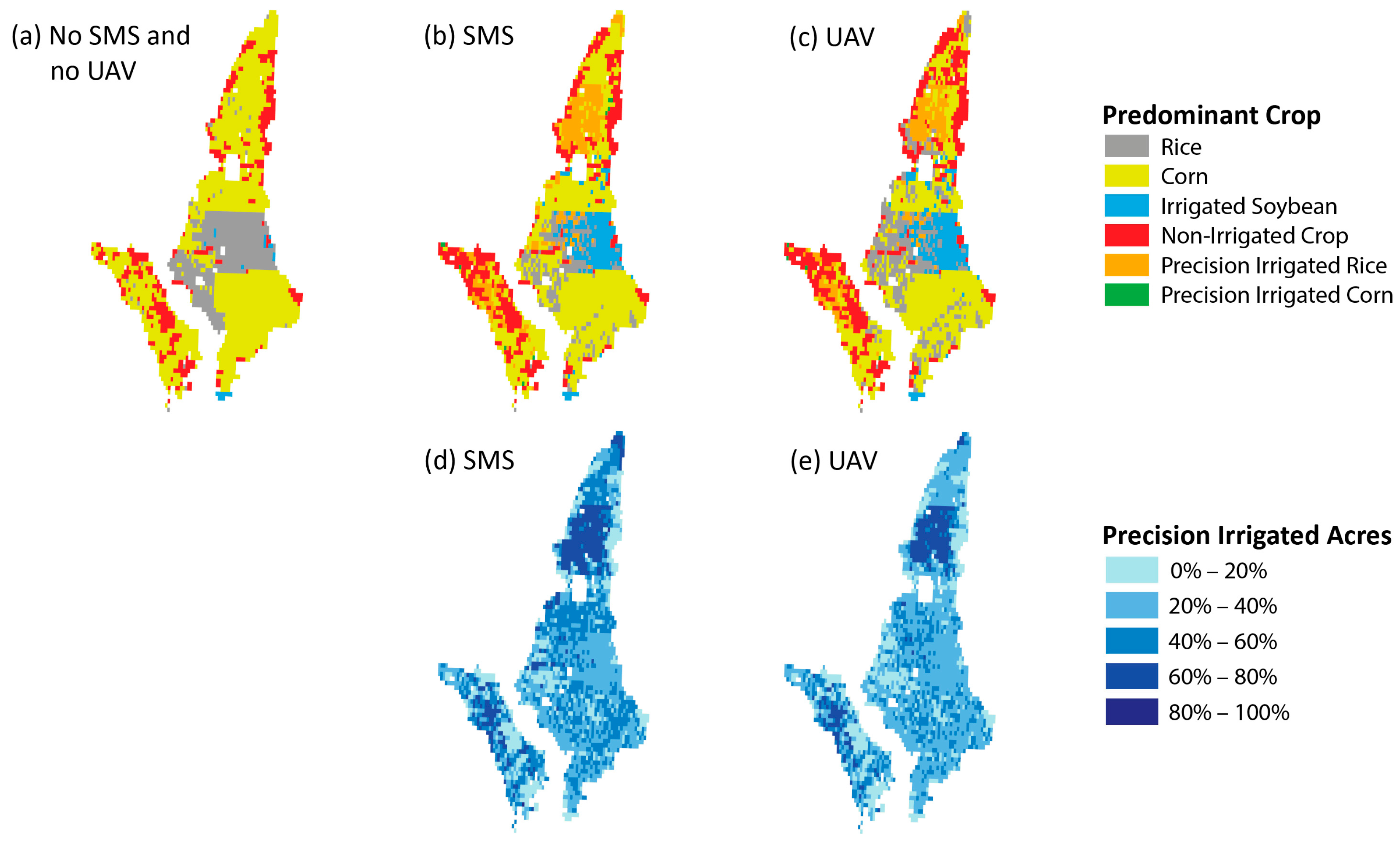
Notes: SMS: Soil-moisture sensors; UAV: Unmanned aerial vehicles; PI: precision irrigation.

indicates the results of the baseline model without precision irrigation or reservoirs. The relative prices over the last 5 years make rice and corn the predominant crops on the landscape at the end of the study period (Figure 2a), and both are irrigation intensive crops. This makes the aquifer decline from 76 million acre-feet to 48.2 million acre-feet in 2045, and the 30-year farm net returns are $5.22 billion. We compare these results with a landscape where farms adopt soil moisture sensors or unmanned aerial vehicles to reduce the costly application of irrigation water. The use of soil moisture sensors increases the amount of land in rice from 305 thousand acres to 343 thousand acres, and most of the rice acreage adopts soil moisture sensors to mitigate irrigation costs (Figure 2b). The increase in rice acreage is accompanied by a decline in corn, cotton, soybean, and non-irrigated sorghum acres. Although rice acreage expands, the soil moisture sensors mean less well pumping, and the aquifer in the final period is close to 48.7 million acre-feet. Figure 2d,e depicts the extent of precision irrigation adoption under each scenario.

The use of unmanned aerial vehicles increases rice acreage to only 316 thousand acres because of the lower irrigation efficiency compared to soil moisture sensors, and much of the rice remains in conventional irrigation. There is a slight decline in the acres of corn, cotton, double crop soybean, and non-irrigated sorghum compared to the baseline (Figure 2c). The final aquifer volume is 48.6 million acre-feet, slightly lower than the 48.7 million acre-feet with the soil moisture sensors, but higher than the 48.2 million acre-feet baseline. The soil moisture sensors have greater net returns per acre-foot conserved than the unmanned aerial vehicles, $9.09 per acre-foot versus $7.69 per acre-foot, because high-value rice acreage increases more with the soil sensors. The soil moisture sensor technology is more expensive per acre, though, and this makes it a less cost-effective solution for aquifer retention than the unmanned aerial vehicles. The positive net returns indicate that both farmers and conservationists gain from the technologies. Though the utility of unmanned aerial vehicles for precision management through mapping crop water stress has been demonstrated [57,58,59,60,61], and plant-based monitoring of water stress to automate variable-rate irrigation has shown the ability to improve irrigation water use [14], systematic and multidisciplinary research is still necessary to verify and quantify improvements from managing crop inputs based on images from unmanned aerial vehicles [61,65].

The presence of on-farm reservoirs and tail-water recovery increases the land in rice and corn compared to the baseline, and the non-irrigated sorghum is nearly gone. When the soil moisture sensors are adopted on the landscape rice increases to 390 thousand acres, corn falls to 672 thousand acres, and the acres in both non-irrigated crop and in reservoirs falls. The aquifer level in the final period rises to 50.4 million acre-feet from 50.2 million acre-feet without the soil moisture sensors. If unmanned aerial vehicles are adopted on the landscape with reservoirs, then the rice acres rise slightly to 357 thousand acres, and the corn acres fall to 678 thousand acres. The acres in reservoirs and non-irrigated sorghum are virtually unchanged from the landscape with reservoirs but without the unmanned aerial vehicles. The aquifer volume increased slightly over the baseline with 50.3 million acre-feet in the final period.

The net returns per acre-foot are higher for the precision irrigation when reservoirs are used on the landscape. This is because more crops use irrigation when reservoirs provide surface water. The farm returns to irrigation that is more efficient and the aquifer retention are magnified by precision irrigation when more of the landscape is using irrigation than before. The net returns per acre are $62 per acre-foot for the soil moisture sensors and $31 per acre-foot for the unmanned aerial vehicles. Looking only at cost-effectiveness for an acre-foot of aquifer retention, though, the unmanned aerial vehicles are preferred since the technology is somewhat less expensive.

The cost and irrigation efficiency of the soil moisture sensors and unmanned aerial vehicles is not known with certainty. We use a low and high-end range for the cost and irrigation efficiency of the precision irrigation technologies to see how crop choice, well pumping, and the farm net returns are affected in

Table 5. Sensitivity analysis of the costs and irrigation efficiency of precision irrigation on land and water use in 2045, and 30-year economic returns.

Land, Water, and Economic Conditions	No SMS and No UAV	Low Cost/High IE SMS	High Cost/Low IE SMS	Low Cost/High IE UAV	High Cost/Low IE UAV
Land use (1000 acres)
Rice—conventional irrigation	305	91	99	90	231
Rice—PI	-	361	232	340	73
Irrigated soybeans—conventional irrigation	3	0	2	0	6
Irrigated soybeans—PI	-	-	-	-	-
Irrigated corn—conventional irrigation	620	282	349	311	363
Irrigated corn—PI	-	254	265	242	255
Irrigated cotton—conventional irrigation	63	34	48	39	56
Irrigated cotton—PI	-	18	9	12	7
Double crop soybean/wheat—conventional irrigation	30	23	29	25	30
Double crop soybean/wheat—PI	-	-	-	-	-
Non-irrigated soybeans	-	-	-	-	-
Non-irrigated sorghum	121	79	108	81	121
Reservoirs	-	-	-	-	-
Water use (1000 ac-ft./year)
Annual groundwater use	1448	1295	1433	1338	1437
Aquifer	48,210	50,240	48,560	49,770	48,390
30 year farm net returns (million $)	5219	5402	5222	5328	5220
Cost effectiveness ($/ac-ft.)	-	148	486	110	365
Net returns per ac-ft. ($/ac-ft.)	-	90	8.57	70	5.55

Notes: SMS: Soil-moisture sensors; UAV: Unmanned aerial vehicles; PI: precision irrigation; IE: Irrigation efficiency.

. For the soil moisture sensors, rice expands to 452 thousand acres for the low cost/high irrigation efficiency scenario while the high cost/low irrigation efficiency scenario has rice expand to just 331 thousand acres. The large expansion of rice in the low cost/high irrigation efficiency scenario makes corn and other crop acreage fall compared to the baseline, and even though more irrigation intensive rice is grown, the well pumping falls to 1422 thousand acre-feet in the final period because the soil moisture sensors increase irrigation efficiency. The crop mix in the high cost/low irrigation efficiency scenario for the soil moisture sensors is largely the same as the landscape without the soil moisture sensors. The well pumping, though, does fall from the baseline to 1433 thousand acre-feet in the final period because of soil moisture sensor adoption.

These crop and water use changes on the landscape from the soil moisture sensor use make the 30-year farm net returns edge up slightly with the high cost/low irrigation efficiency scenario and go up substantially to $5.40 billion in the low cost/high irrigation efficiency scenario. The aquifer rises to 50.2 million acre-feet in the low cost/high irrigation efficiency scenario and to just 48.6 million acre-feet in the high cost/low irrigation efficiency scenario. The net-benefit assessment indicates $90 per acre-foot if the soil moisture sensors are low cost and high efficiency, and a modest $8.57 per acre-foot for high cost and low efficiency sensors. This means there is a wide range of potential net returns to an optimized landscape allowing the use of soil moisture sensors, but implementation that more closely approximates the low cost/high irrigation efficiency scenario can generate substantial gains to both farmers and the aquifer. The use of unmanned aerial vehicles makes the rice acreage expand to 430 thousand acres in the low cost/high irrigation efficiency scenario but fall slightly to 304 thousand acres in the high cost/low irrigation efficiency scenario. The low cost/high irrigation efficiency scenario for unmanned aerial vehicles has 1338 thousand acre-feet of well pumping in the final period because the unmanned aerial vehicles allow for a reduction in water use even as rice acres expand. There are 1437 thousand acre-feet of well pumping in the final period for the high cost/low efficiency scenario, only slightly below the baseline, because there is limited adoption of the unmanned aerial vehicles when the irrigation efficiency is low. The aquifer rises to 49.7 million acre-feet and 30-year farm net returns rise to $5.3 billion in the low cost/high efficiency scenario; however, the aquifer rises to only 48.4 million acre-feet and $5.2 billion in 30-year farm net returns for the high cost/low irrigation efficiency scenario. The wide range in the net returns per acre-foot for the low and high-end scenarios, from $70 to $5.55 per acre-foot, for the unmanned aerial vehicles indicates, as for the soil sensors, that improving the efficiency of the technology is valuable for profitability and aquifer retention.

The use of cost-share assistance to encourage precision irrigation, shown in

Table 6. Water conservation policies influence on aquifer, and economic returns, government revenue, and groundwater conservation cost.

Policy	Aquifer, 2045 (Thousand Acre-Feet)	Farm Net Returns, 30 Year NPV a ($ Millions)	Government Revenue, 30 Year NPV ($ Millions)	Groundwater Conservation Cost b ($ Per Acre-Foot)
Baseline	48,210	5219	-	-
Cost share on soil moisture sensors c	49,140	5231	−67	$59
Cost share on unmanned aerial vehicles c	48,540	5231	−34	$67
Cap on groundwater use d	49,510	5204	-	$12
Fee on groundwater use d	49,430	5150	2	$1.6

Notes: All allow on-farm reservoirs. ^a The farm net returns include the payments to or receipts from the government because of the policy; ^b Groundwater conservation cost is calculated as the policy cost (which is the farm net returns in the baseline less the farm net returns plus government revenue for each policy scenario) divided by the change in aquifer level between the policy option and the baseline; ^c The cost share is 60% for soil moisture sensors and unmanned aerial vehicles based on the rates from the Natural Resource Conservation Service’s (NRCS) Agricultural Water Enhancement Program [33]; ^d We choose a cap on groundwater pumping (220% of initial pumping levels) and a fee on groundwater pumping costs (4%) to achieve groundwater conservation similar to the cost share on soil moisture sensors.

, improves farm net returns over 30 years and increases the volume of the aquifer, but the subsidy represents a loss of government revenue that the taxpayer must bear. The policies result in a loss of economic value to society because the rise in farm net returns is less than the loss in government revenue. However, these polices allow more of the aquifer to be retained. The groundwater conservation cost per acre-foot for the study period is found by dividing the economic cost to society of the policy by the acre-feet of the aquifer conserved. The soil moisture sensors are more irrigation-efficient and only slightly more expensive than the unmanned aerial vehicles, and this makes the $59 groundwater conservation cost per acre-foot for the cost-share on the soil moisture sensors less than the $67 cost per acre-foot for the unmanned aerial vehicles. The cost-share policies are both expensive, however, compared to the groundwater conservation cost associated with policies such as a cap on groundwater use ($12/acre-foot) or a fee on groundwater use ($1.6 acre-foot). Policies that target groundwater use directly through a cap or tax appear more cost-effective at groundwater conservation than the policies that offer a cost-share on irrigation technology for crops such as cotton and soybeans that are not especially irrigation intensive.

4. Discussion

Our results support the conclusion that remote monitoring to inform variable-rate irrigation practices is an increasingly viable alternative for reducing groundwater depletion through precision agriculture. We demonstrate that remote monitoring to inform variable-rate irrigation can improve irrigation efficiency modestly enough to conserve aquifer volumes, reduce pumping costs, and increase net returns by still allowing for more production of profitable but water-intensive rice. Furthermore, our results indicate the potential of remote monitoring and variable-rate irrigation to provide benefits in tandem with other complimentary practices such as the use of the on-farm reservoirs.

The uncertainty around the cost and water-use efficiency of the remote sensing techniques suggest that the net-returns per acre-foot of aquifer retention could be significantly larger or a little lower than the baseline costs and water use efficiencies for the precision irrigation techniques suggest. As the costs of the sensors fall and the efficiencies continue to improve, then the net returns per acre-foot of conserved aquifer promise to become substantially larger. As an important reminder, our model makes the simplifying assumption that all reduction in applied water due to improved irrigation efficiency saves irrecoverable fractions of applied irrigation water. While the overwhelming proportion of annual recharge to the alluvial aquifer is the result of precipitation and surface water flux [37], precision irrigation scenarios may overestimate the aquifer volume by failing to account for decreased levels of deep percolation over the long term.

A cost-share policy to encourage more adoption of the sensing technologies appears to incur greater costs on society than either a regulatory cap of groundwater use or tax on groundwater use. Leaving aside issues surrounding an equitable share of the conservation burden across the agricultural producers and the rest of society, the most efficient approach to conservation is through directly targeting the overused resource with a cap or a tax.

The evaluation of benefits and costs here between soil moisture sensors and unmanned aerial vehicles only considers increased performance in irrigation efficiency with respect to soil-based versus plant-based monitoring regimes. We do not consider other benefits of variable-rate irrigation or other applications of remote monitoring which might present other benefits. Another implication of targeted spatial application of irrigation is that nutrient and sediment runoff is minimized, improving the quality of surface waters [66]. In addition, it may be possible to monitor a range of other plant conditions with unmanned aerial vehicles at little additional cost that are not able to be measured by wireless soil moisture sensors [24]. Explicit spatial management of other crop conditions might even allow farmers to realize more fully the benefits of high spatial resolution monitoring. For instance, producers may be able to improve the efficiency of nutrient application and uptake in a way that both lowers costs and increases yield. Although many farms may already have spatial soil information, we do not know how many have this information or how many use any form of precision agriculture. To be conservative in the adoption rates of this technology, we attribute all the costs of this spatial soil information to the soil sensors. To the extent most farmers already have this information, the soil moisture sensors will be more profitable than we have indicated.

The soil sensor technologies resemble a constant return to scale technology more than other irrigation equipment like center pivots or on-farm reservoirs. This is because soil sensors only have a particular spatial radius where they are effective. However, the unmanned aerial vehicle technologies do exhibit economies of scale, and the unquestionable improvement in these technologies is likely to further increase consolidation in the farming sector. The average farm size in the region has risen from 750 acres in 2002 to 820 acres in 2012 [35]. Improved sensing technologies are likely to augment this trend.

As costs associated with unmanned aerial vehicles or their services decrease and monitoring applications increase, the aircraft are likely to surpass soil moisture sensors in terms of both cost-effectiveness of aquifer savings and net returns. Given that the most attractive policy alternative among the farming community also comes at the greatest cost to society, it may be that widespread implementation of one of these practices depends on a continued drop in costs. Future work should continue to explore the role of precision technology and high-resolution monitoring in agriculture by giving needed attention to adapting best practices to region-specific constraints. Toward this goal, it will be important to continue to characterize the benefits and costs of these applications under different environmental and economic conditions.

References

1. Schaible, G.; Aillery, M. Water Conservation in Irrigated Agriculture: Trends and Challenges in the Face of Emerging Demands; United States Department of Agriculture (USDA), Economic Research Service (ERS): Washington, DC, USA, 2012.
2. Arkansas Water Plan Update. 2014. Available online: http://arkansaswaterplan.org/plan/ArkansasWaterPlan/Update.htm (accessed on 10 June 2016).
3. Canessa, P.; Green, S.; Zoldoske, D. Agricultural Water Use in California: A 2011 Update; Staff Report; The Center for Irrigation Technology, Fresno State University: Fresno, CA, USA, 2011. Available online: http://www.waterboards.ca.gov/waterrights/water_issues/programs/hearings/cachuma/exbhts_2012feir/cachuma_feir_mu289.pdf (accessed on 2 December 2016).
4. Allen, R.G.; Willardson, L.S.; Burt, C.; Clemmens, A.J. Water conservation questions and definitions from a hydrologic perspective. In Proceedings of the IA International Irrigation Show, San Diego, CA, USA, 18 November 2003.
5. Snyder, R.L.; Hanson, B.R.; Coppock, R. How Farmers Irrigate in California; University of California Division of Agriculture and Nature Research: Davis, CA, USA, 1986; pp. 1–6. Available online: http://anrcatalog.ucanr.edu/pdf/21414e.pdf (accessed on 2 December 2016).
6. Hedley, C.B.; Yule, I.J. Soil water status mapping and two variable-rate irrigation scenarios. Precis. Agric. 2009, 10, 342–355. [Google Scholar] [CrossRef]
7. Hedley, C.B.; Yule, I.J.; Tuohy, M.P.; Vogeler, I. Key performance indicators for simulated variable-rate irrigation of variable soils in humid regions. Trans. ASABE 2009, 52, 1575–1584. [Google Scholar] [CrossRef]
8. Hedley, C.B.; Bradbury, S.; Ekanayake, J.; Yule, I.J.; Carrick, S. Spatial irrigation scheduling for variable rate irrigation. In Proceedings of the New Zealand Grassland Association Conference, Lincoln, New Zealand, 15–18 November 2010; New Zealand Grassland Association: Dunedin, New Zealand, 2010; Volume 72, pp. 97–102. [Google Scholar]
9. Hedley, C.B.; Yule, I.J.; Bradbury, S. Analysis of potential benefits of precision irrigation for variable soils at five pastoral and arable production sites in New Zealand. In Proceedings of the 19th World Soil Congress, Brisbane, Australia, 1–6 August 2010; pp. 1–6.
10. Thrikawala, S.; Weersink, A.; Fox, G.; Kachanoski, G. Economic feasibility of variable-rate technology for nitrogen on corn. Am. J. Agric. Econ. 1999, 81, 914–927. [Google Scholar] [CrossRef]
11. Zhang, M.; Li, M.; Wang, W.; Liu, C.; Gao, H. Temporal and spatial variability of soil moisture based on WSN. Math. Comput. Model. 2013, 58, 826–833. [Google Scholar] [CrossRef]
12. Lowenberg-DeBoer, J. Economics of variable rate planting for corn. In Precision Agriculture; ASA, CSSA, SSSA: Madison, WI, USA, 1999; pp. 1643–1651. [Google Scholar]
13. Strickland, R.M.; Ess, D.R.; Parsons, S.D. Precision farming and precision pest management: The power of new crop production technologies. J. Nematol. 1998, 30, 431–435. [Google Scholar] [PubMed]
14. Peters, R.T.; Evett, S.R. Automation of a center pivot using the temperature-time-threshold method of irrigation scheduling. J. Irrig. Drain. Eng. 2008, 134, 286–291. [Google Scholar] [CrossRef]
15. LaRue, J.L. Variable Rate Irrigation 2010 Field Results for Center Plains Conference. In Proceedings of the 23rd Annual Central Plains Irrigation Conference, Burlington, CO, USA, 22–23 February 2011; p. 135.
16. Stone, K.C.; Bauer, P.J.; Busscher, W.J.; Millen, J.A.; Evans, D.E.; Strickland, E.E. Variable-rate irrigation management using an expert system in the eastern coastal plain. Irrig. Sci. 2015, 33, 167–175. [Google Scholar] [CrossRef]
17. Barnes, E.M.; Sudduth, K.A.; Hummel, J.W.; Lesch, S.M.; Corwin, D.L.; Yang, C.; Daughtry, C.S.; Bausch, W.C. Remote-and ground-based sensor techniques to map soil properties. Photogramm. Eng. Remote Sens. 2003, 69, 619–630. [Google Scholar] [CrossRef]
18. O’Shaughnessy, S.A.; Evett, S.R.; Andrade, A.; Workneh, F.; Price, J.A.; Rush, C.M. Site-specific variable-rate irrigation as a means to enhance water use efficiency. In Proceedings of the Joint ASABE/IA Irrigation Symposium: Emerging Technologies for Sustainable Irrigation, Long Beach, CA, USA, 10–12 November 2015.
19. Longchamps, L.; Khosla, R.; Reich, R.; Gui, D.W. Spatial and temporal variability of soil water content in leveled fields. Soil Sci. Soc. Am. J. 2015, 79, 1446–1454. [Google Scholar] [CrossRef]
20. Starr, G.C. Assessing temporal stability and spatial variability of soil water patterns with implications for precision water management. Agric. Water Manag. 2005, 72, 223–243. [Google Scholar] [CrossRef]
21. Hedley, C.B.; Yule, I.J. A method for spatial prediction of daily soil water status for precise irrigation scheduling. Agric. Water Manag. 2009, 96, 1737–1745. [Google Scholar] [CrossRef]
22. Schmitz, M.; Kuyper, M.C. Soil moisture sensors in field application, a comparative study. Z. Bewässerungswissenschaft 1998, 33, 87–102. [Google Scholar]
23. Schmitz, M.; Sourell, H. Variability in soil moisture measurements. Irrig. Sci. 2000, 19, 147–151. [Google Scholar] [CrossRef]
24. Stombaugh, T.; Smith, S.; Thamann, M. The Use of Unmanned Aircraft Systems in Agriculture; Biosystems and Agricultural Engineering Update; Cooperative Extension Service, University of Kentucky: Lexington, KY, USA, 2015. [Google Scholar]
25. Federal Aviation Administration. Press Release—DOT and FAA Finalize Rules for Small Unmanned Aircraft Systems. Available online: https://www.faa.gov/news/press_releases/news_story.cfm?newsId=20515 (accessed on 5 September 2016).
26. Moffet, C. Unmanned Aerial Vehicles Advance Agriculture. The Samuel Roberts Noble Foundation, August 2014. Available online: www.noble.org/ag/research/uavs-advance-ag/ (accessed on 5 September 2016).
27. Kovacs, K.; Popp, M.; Brye, K.; West, G. On-farm reservoir adoption in the presence of spatially explicit groundwater use and recharge. J. Agric. Resour. Econ. 2015, 40, 23–49. [Google Scholar]
28. Seaber, P.R.; Kapinos, F.P.; Knapp, G.L. Hydrologic Unit Maps; Water Supply Paper; United States Government Publishing Office: Washington, DC, USA, 1987.
29. Division of Agriculture-University of Arkansas. 2012 Crop and Enterprise Budgets. Available online: http://www.uaex.edu/depts/ag_economics/budgets/2012/Budgets2012.pdf (accessed on 25 July 2013).
30. Clark, B.R.; Westerman, D.A.; Fugitt, D.T. Enhancements to the Mississippi Embayment Regional Aquifer Study (MERAS) Groundwater-Flow Model and Simulations of Sustainable Water-Level Scenarios; U.S. Geological Survey: Reston, VA, USA, 2013.
31. Arkansas Natural Resources Commission (ANRC). Arkansas Groundwater Protection and Management Report for 2011; ANRC: Little Rock, AR, USA, 2012.
32. GAMS Development Corporation. Generalized Algebraic Modeling System (23.5.2) [Software]; GAMS Development Corporation: Washington, DC, USA, 2010. [Google Scholar]
33. Natural Resources Conservation Service (NRCS). 2014 EQIP Conservation Practices and Payment Rates. Available online: http://www.nrcs.usda.gov/wps/portal/nrcs/detail/ar/home/?cid=stelprdb1240703 (accessed on 13 August 2014).
34. Johnson, D.M.; Mueller, R. The 2009 Cropland Data Layer. Photogramm. Eng. Remote Sens. 2010, 1201–1205. [Google Scholar]
35. U.S. Department of Agriculture (USDA)-National Agricultural Statistics Service (NASS). Soybean Irrigated and Non-Irrigated. Available online: http://www.nass.usda.gov/Statistics_by_State/Arkansas/Publications/County_Estimates/ (accessed on 10 November 2012).
36. U.S. Department of the Treasury. Interest Rate Statistics. Available online: http://www.treasury.gov/resource-center/data-chart-center/interest-rates/Pages/default.aspx (accessed on 13 December 2012).
37. Reed, T.B. Recalibration of a Ground-Water Flow Model of the Mississippi River Valley Alluvial Aquifer of Northeastern Arkansas, 1918–1998, with Simulations of Water Levels Caused by Projected Ground-Water Withdrawals through 2049; U.S. Department of the Interior, U.S. Geological Survey: Reston, VA, USA, 2003.
38. Yohannes, F.; Tadesse, T. Effect of drip and furrow irrigation and plant spacing on yield of tomato at Dire Dawa, Ethiopia. Agric. Water Manag. 1998, 35, 201–207. [Google Scholar] [CrossRef]
39. Kebede, H.; Fisher, D.K.; Sui, R.; Reddy, K.N. Irrigation methods and scheduling in the delta region of Mississippi: Current status and strategies to improve irrigation efficiency. Am. J. Plant Sci. 2014, 5, 2917–2928. [Google Scholar] [CrossRef]
40. CALFED. Final Report—Water Use Efficiency Comprehensive Evaluation. CALFED Bay-Delta Program Water Use Efficiency Element. 2006. Available online: http://www.calwater.ca.gov/content/Documents/library/WUE/2006_WUE_Public_Final.pdf (accessed on 2 December 2016). [Google Scholar]
41. Pfeiffer, L.; Lin, C.-Y.C. Does efficient irrigation technology lead to reduced groundwater extraction? Empirical evidence. J. Environ. Econ. Manag. 2014, 67, 189–208. [Google Scholar] [CrossRef]
42. Flanders, A.; Baker, R.; Barber, T.; Faske, T.; Ginn, H.; Grimes, C.; Hardke, J.; Lawson, K.; Lorenz, G.; Mazzanti, R.; et al. 2014 Crop Production Budgets for Farm Planning; University of Arkansas Cooperative Extension Service, Division of Agriculture: Little Rock, AR, USA, 2014; Available online: http://www.uaex.edu/farm-ranch/economics-marketing/farm-planning/budgets/crop-budgets.aspx (accessed on 15 January 2015).
43. Great Pacific Trading Company (GPTC). Charts and Quotes. Available online: http://www.gptc.com/quotes.html (accessed on 20 November 2012).
44. U.S. Department of Agriculture (USDA) Farm Service Agency (FSA). Conservation Reserve Program Statistics. Available online: http://www.fsa.usda.gov/programs-and-services/conservation-programs/reports-and-statistics/conservation-reserve-program-statistics/index (accessed on 14 June 2015).
45. Hogan, R.; Stiles, S.; Tacker, P.; Vories, E.; Bryant, K.J. Estimating Irrigation Costs. Available online: http://www.uaex.edu/Other_Areas/publications/pdf/FSA-28.pdf (accessed on 10 July 2010).
46. Energy Information Administration (EIA); U.S. Department of Energy. Gasoline and Diesel Fuel Update. Available online: http://www.eia.gov/petroleum/gasdiesel/ (accessed on 20 November 2012).
47. Smartt, J.H.; Wailes, E.J.; Young, K.B.; Popp, J.S. MARORA (Modified Arkansas Off-Stream Reservoir Analysis) Program Description and User’s Guide; University of Arkansas: Fayetteville, AR, USA, 2002; unpublished manuscript; Available online: http://agribus.uark.edu/2893.php (accessed on 28 April 2013).
48. Young, K.B.; Wailes, E.J.; Popp, J.H.; Smartt, J. Value of water conservation improvements on Arkansas rice farms. J. ASFMRA 2004, 67, 119–126. [Google Scholar]
49. Hedley, C.; Craigie, R.; Bradbury, S. Variable Rate Irrigation for Improved Water Use Efficiency; Final Report Sustainable Farming Fund Project; Landcare Research: Lincoln, New Zealand, 2013. [Google Scholar]
50. Vories, E.; Tacker, P.; Stephenson, D.; Bajwa, S.; Perry, C. Performance of a variable-rate center pivot system. In Proceedings of the World Water and Environment Resources Congress, Honolulu, HI, USA, 12–16 May 2008.
51. Camp, C.R.; Sadler, E.J.; Evans, R.G. Precision water management: Current realities, possibilities, and trends. In Handbook of Precision Agriculture; CRC Press: Boca Raton, FL, USA, 2006; pp. 153–183. [Google Scholar]
52. Meron, M.; Tsipris, J.; Orlov, V.; Alchanatis, V.; Cohen, Y. Crop water stress mapping for site-specific irrigation by thermal imagery and artificial reference surfaces. Precis. Agric. 2010, 11, 148–162. [Google Scholar] [CrossRef]
53. Evett, S.R.; O’Shaughnessy, S.A.; Colaizzi, P.D.; Schwartz, R.C. Soil water sensing: Implications of sensor capabilities for variable rate irrigation management. In Proceedings of the IA Exposition and Technical Conference, Fairfax, VA, USA, 17–21 November 2014.
54. Olson, J. New Soil Maps Spark Change. Farm Industry News. 1 March 2000. Available online: http://farmindustrynews.com/new-soil-maps-spark-change (accessed on 8 July 2016).
55. Vellidis, G.; Tucker, M.; Perry, C.; Kvien, C.; Bednarz, C. A real-time wireless smart sensor array for scheduling irrigation. Comput. Electron. Agric. 2008, 61, 44–50. [Google Scholar] [CrossRef]
56. U.S. Department of Agriculture (USDA)—Natural Resource Conservation Service (NRCS). Cost Scenarios 442 Sprinkler System. Available online: https://efotg.sc.egov.usda.gov/references/public/KS/CostSenarios_442SprinklerSystem.pdf (accessed on 8 July 2016).
57. Herwitz, S.R.; Johnson, L.F.; Dunagan, S.E.; Higgins, R.G.; Sullivan, D.V.; Zheng, J.; Lobitz, B.M.; Leung, J.G.; Gallmeyer, B.A.; Aoyagi, M.; et al. Imaging from an unmanned aerial vehicle: Agricultural surveillance and decision support. Comput. Electron. Agric. 2004, 44, 49–61. [Google Scholar] [CrossRef]
58. Berni, J.A.; Zarco-Tejada, P.J.; Suárez, L.; Fereres, E. Thermal and narrowband multispectral remote sensing for vegetation monitoring from an unmanned aerial vehicle. IEEE Trans. Geosci. Remote Sens. 2009, 47, 722–738. [Google Scholar] [CrossRef]
59. Berni, J.A.J.; Zarco-Tejada, P.J.; Sepulcre-Cantó, G.; Fereres, E.; Villalobos, F. Mapping canopy conductance and CWSI in olive orchards using high resolution thermal remote sensing imagery. Remote Sens. Environ. 2009, 113, 2380–2388. [Google Scholar] [CrossRef]
60. Xiang, H.; Tian, L. Development of a low-cost agricultural remote sensing system based on an autonomous unmanned aerial vehicle (UAV). Biosyst. Eng. 2011, 108, 174–190. [Google Scholar] [CrossRef]
61. Shi, Y.; Thomasson, J.A.; Murray, S.C.; Pugh, N.A.; Rooney, W.L.; Shafian, S.; Rajan, N.; Rouze, G.; Morgan, C.L.; Neely, H.L.; et al. Unmanned aerial vehicles for high-throughput phenotyping and agronomic research. PLoS ONE 2016, 11, e0159781. [Google Scholar] [CrossRef] [PubMed]
62. Ireland-Otto, N.; Ciampitti, I.; Blanks, M.; Burton, R.; Balthazor, T. Costs of Using Unmanned Aircraft on Crop Farms. J. ASFMRA 2016, 130–148. [Google Scholar]
63. Lo, T.H. Quantification of Variable Rate Irrigation Benefits and Spatial Variability in Root Zone Water Holding Capacity. Master’s Thesis, University of Nebraska, Lincoln, NE, USA, 2015. [Google Scholar]
64. Evans, R.G.; LaRue, J.; Stone, K.C.; King, B.A. Adoption of site-specific variable rate sprinkler irrigation systems. Irrig. Sci. 2013, 31, 871–887. [Google Scholar] [CrossRef]
65. Zhang, C.; Kovacs, J.M. The application of small unmanned aerial systems for precision agriculture: A review. Precis. Agric. 2012, 13, 693–712. [Google Scholar] [CrossRef]
66. United States Environmental Protection Agency (EPA). National Management Measure to Control Nonpoint Source Pollution from Agriculture; EPA: Washington, DC, USA, 2003.
Figure 1. Three eight-digit hydrologic unit code (HUC) watersheds in the Mississippi Delta region of eastern Arkansas define the outer boundary of the study area. An eight-digit HUC defines the drainage area of the sub-basin of a river. County lines overlay the study area. Public land and urban areas are excluded. The location of the study area within the state of Arkansas is shown.
Water 09 00028 g001
Figure 2. Predominant crops grown on the landscape in: (a) the baseline (No SMS and no UAV); and with precision irrigation using (b) soil moisture sensors (SMS); or (c) unmanned aerial vehicles (UAV). Non-irrigated crops and precision irrigated rice replace corn when remote sensing techniques are adopted. The percent of cropland using precision irrigation is shown when the remote sensing technique is: (d) soil moisture sensors; and (e) unmanned aerial vehicles. The percentage of precision irrigated cropland is higher in the northern and western sections of the landscape where the aquifer is more depleted.
Water 09 00028 g002