SWAT Modeling for Depression-Dominated Areas: How Do Depressions Manipulate Hydrologic Modeling?

Abstract

Modeling hydrologic processes for depression-dominated areas such as the North American Prairie Pothole Region is complex and reliant on a clear understanding of dynamic filling-spilling-merging-splitting processes of numerous depressions over the surface. Puddles are spatially distributed over a watershed and their sizes, storages, and interactions vary over time. However, most hydrologic models fail to account for these dynamic processes. Like other traditional methods, depressions are filled as a required preprocessing step in the Soil and Water Assessment Tool (SWAT). The objective of this study was to facilitate hydrologic modeling for depression-dominated areas by coupling SWAT with a Puddle Delineation (PD) algorithm. In the coupled PD-SWAT model, the PD algorithm was utilized to quantify topographic details, including the characteristics, distribution, and hierarchical relationships of depressions, which were incorporated into SWAT at the hydrologic response unit (HRU) scale. The new PD-SWAT model was tested for a large watershed in North Dakota under real precipitation events. In addition, hydrologic modeling of a small watershed was conducted under two extreme high and low synthetic precipitation conditions. In particular, the PD-SWAT was compared against the regular SWAT based on depressionless DEMs. The impact of depressions on the hydrologic modeling of the large and small watersheds was evaluated. The simulation results for the large watershed indicated that SWAT systematically overestimated the outlet discharge, which can be attributed to the failure to account for the hydrologic effects of depressions. It was found from the PD-SWAT modeling results that at the HRU scale surface runoff initiation was significantly delayed due to the threshold control of depressions. Under the high precipitation scenario, depressions increased the surface runoff peak. However, the low precipitation scenario could not fully fill depressions to reach the overflow thresholds in the selected sub-basins. These results suggest the importance of depressions as gatekeepers in watershed modeling.

1. Introduction

The North American Prairie Pothole Region (PPR) can be typified by the presence of numerous potholes and the associated wetlands [1]. However, due to a series of complexities related to these depressions and their characteristics (e.g., hydrologic connectivity of depressions), hydrologic modeling for the PPR is a challenging task [2]. Different studies have been conducted to address the depression storage effects and simulate the characteristics of depression-dominated areas [3,4,5,6,7,8,9]. For example, Chu et al. [6] developed a physically based hydrologic model which took the dynamic variations of puddles into account. The puddle-to-puddle (P2P) model incorporated the Puddle Delineation (PD) algorithm [5] to obtain detailed characteristics of depressions and simulate the real microtopography-controlled P2P overland flow, as well as infiltration and unsaturated flow [6]. It provided all details on the cell to cell and puddle to puddle overland flow processes, puddle filling, spilling, merging, and splitting dynamics, spatial and temporal distributions of ponded water, variations in hydrologic connectivity, and discharges at basin outlets [6]. The P2P model has been tested for various laboratory and field surfaces, including a site in the PPR, which highlighted the significance of the dynamic P2P processes and threshold behavior of potholes [7,9].

The Soil and Water Assessment Tool (SWAT) model [10,11] has been extensively used for evaluating watershed-scale water quantity and quality problems [12,13,14]. In particular, ArcSWAT [15], an extension of ArcGIS, facilitates SWAT modeling by providing a user-friendly interface for DEM-based watershed delineation, processing of land use and soil type GIS data, HRU definition, meteorological data analysis, and preparation of SWAT input datasets. As a preprocessing procedure of delineation in ArcSWAT, all depressions are filled or removed to generate well-connected drainage networks [2]. Therefore, in SWAT applications, different assumptions are often introduced for depressions. For example, Sophocleous et al. [16] considered depressions as non-contributing areas. Shrestha et al. [17] assumed that for all rainfall events, 100% of the depressional areas contributed runoff to the outlet. These studies did not consider the real dynamic P2P processes of depressions and their effects on hydrologic modeling. Thus, these approaches are may not be applicable to the PPR landscapes.

To enhance the capabilities of SWAT for various complex conditions, some modified SWAT models have been developed. For instance, Yactayo [18] developed SWAT-karst by accounting for the unique relationship between surface water and groundwater in karst environments at a HRU scale to simulate hydrologic processes and nitrogen transport. Mekonnen et al. [8] incorporated the heterogeneity of depression storage into the SWAT modeling. Their modified model, SWAT-probability distribution landscape distribution (SWAT-PDLD), was calibrated and validated for two watersheds within the PPR of North America [8]. They employed ArcGIS [19] tools to identify depressions, their storage and surface area. The results from the SWAT-PDLD model demonstrated improved estimations of stream flow for the selected watersheds. In addition, Mekonnen et al. [2] developed a modified version of SWAT for sediment export simulation from cold-climate, depression dominated watersheds. They incorporated the seasonal variability of soil erodibility due to the cold-climate conditions into the SWAT-PDLD, tested their model for two depression-dominated watersheds in Canada, and concluded that the simulated sediment export from the case study watersheds was significantly improved by their modified model.

In SWAT modeling, three tools including Potholes, Ponds, and Wetlands can be utilized to account for depressions and their impacts on hydrologic simulation. In most studies, the depression storage is considered as a lumped volume of water by incorporating the wetlands and ponds tools in SWAT [20,21]. Specifically, depressions are incorporated at the sub-basin scale and linked to the routing process in SWAT. However, depression storage is a function of infiltration and other hydrologic processes, and thus the ponds and wetlands tools are not able to represent the real characteristics of depressions [20,21,22].

A fundamental question is: how do depressions manipulate hydrologic modeling? This modeling study was aimed to highlight the threshold-control roles of depressions in depression-dominated areas and to demonstrate the depression-induced changes in modeling results. Specifically, the PD algorithm [5] was used to characterize surface depressions and their hierarchical relationships, and precisely calculate the depression storage and other microtopographic parameters based on digital elevation models (DEMs). The detailed topographic information from the PD was then linked to the pothole tool of the SWAT model at the hydrologic response unit (HRU) scale to provide an improved, coupled PD-SWAT modeling approach. To highlight the significant impacts of depressions in depression-dominated regions, the coupled PD-SWAT was then applied to a large watershed and one of its small sub-basins under both real and two synthetic extreme precipitation conditions. The hypothetical precipitation scenarios were selected to pinpoint the filling-spilling process of depressions under extreme rainfall scenarios. In particular, the new PD-SWAT modeling for the depression-dominated landscapes was compared against the normal SWAT modeling based on the preprocessed depressionless DEMs. In addition, the performances of the PD-SWAT and SWAT models were assessed by using the observed discharge data for the large watershed.

2. Materials and Methods

2.1. Introduction to the PD Algorithm: How to Consider Real Topographic Depressions

The role of depressions across various spatial scales is far beyond the functions of storing and detaining/retaining surface runoff [5]. In this study, an automated PD algorithm [5] was utilized to characterize surface microtopography and precisely compute surface depression storage and other topographic parameters. The PD algorithm comprises of several steps including identification of puddle centers, thresholds, and all other grids included in depressions (puddle cells). These steps lead to identification of the first level puddles over the surface. If two first-level puddles share a common threshold, they potentially merge, forming a second-level puddle. Similarly, further combination of such puddles forms higher level puddles. Following the formation of puddle levels, the hierarchical relationships of the puddles are established, which provides insight into the hydrologic connectivity of puddles and eventually results in a cascaded drainage network. When identification of depressions and their relationships is completed, depression storage capacity and other topographic characteristics are determined for all levels. The outputs from the PD can be incorporated into hydrologic models to account for the dynamic variations of puddles and their impacts on the hydrologic simulation [6]. It should be noted that PD is able to cope with special topographic features, such as flats (i.e., a set of adjacent grids with the same elevation) and multi-threshold depressions (i.e., depressions with two or more thresholds) [5,6].

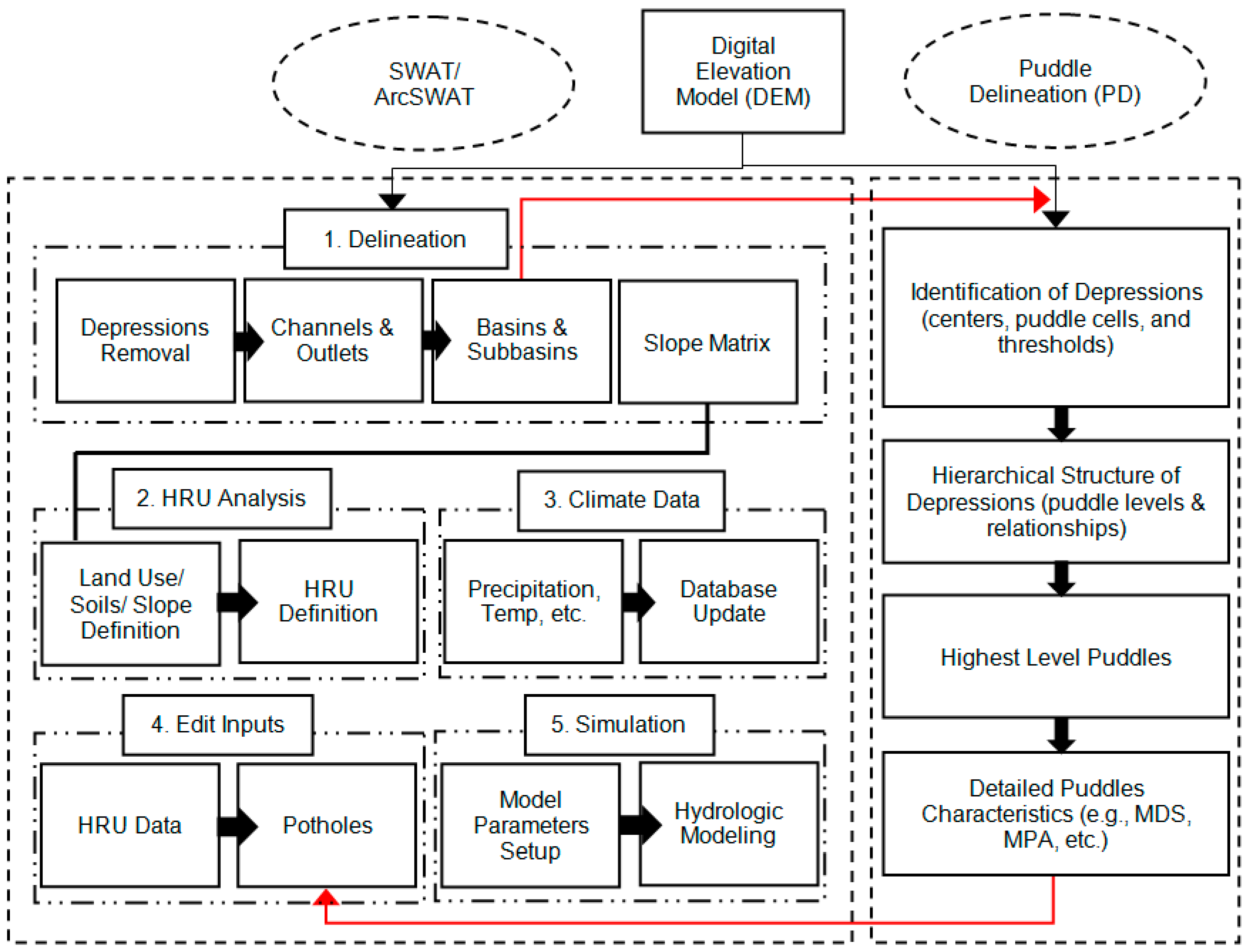
2.2. Coupled PD-SWAT Model

Figure 1 illustrates the fundamental steps of the coupled PD-SWAT modeling system. DEM is the initial input data for the surface delineation process (Figure 1). As a preprocessing step for SWAT modeling, all depressions/sinks are filled. This filling process creates a depressionless DEM (Figure 1). Then, flow directions and accumulations are calculated for all DEM grids; stream channels and outlets are identified; and sub-basin boundaries are eventually determined. Land use/land covers (LULC), soil types, and slope matrix are required input data to construct HRUs for all sub-basins. Each HRU is defined based on a unique combination of LULC, soil type, and slope. The SWAT model simulates the hydrologic processes in all HRUs, which are further aggregated to each sub-basin through the variable storage function routing method [21]. Defining daily meteorological data such as precipitation, minimum/maximum temperatures, humidity, solar radiation, and wind speed, is the third step in the SWAT hydrologic modeling (Figure 1).

Although all depressions are removed in the delineation process, SWAT does provide the Ponds, Wetlands and Potholes tools as a lumped way to compute outflow from the depressions [23,24] and to account for the effect of depressions [21]. Potholes and their parameters can be defined at the HRU scale [23]. However, SWAT cannot compute the required pothole parameters such as ponding area, depression storage, and depth of puddles based on the surface DEM. In this study, to account for the threshold control of depressions and their impacts on SWAT hydrologic modeling, watersheds are divided into a number of sub-basins, each of which is further subdivided into two types of HRUs: (1) depression-dominated HRU and (2) normal depressionless HRUs. The basin and sub-basin boundaries delineated in the SWAT modeling system are transferred to the PD program. Based on the original DEM, PD quantifies surface topography and depression characteristics at the sub-basin and HRU scales (Figure 1). Specifically, PD provides the detailed spatial distribution of depressions, their storages, ponding areas, overflow thresholds, and the hierarchical relationships and connectivity of puddles for different puddle levels. Such topographic details allow the SWAT users to consider a desired number of sub-basins and HRUs. That is, based on the size and distribution of depressions, users can consider more or fewer sub-basins to account for the detailed distribution of depressions or lump them together. The PD program delineates the surface solely based on the DEM. However, many depressions over the surface may not be real ones, but artifacts of elevation variations in the DEM. PD outputs storage, area, mean depth, and other parameters of all depressions. This gives the user options to consider or disregard any identified depressions in the modeling. For example, in this study all the puddles with a mean depth less than 5 cm were not considered.

Based on the detailed hydrotopographic information obtained from the PD program, the pothole features of the SWAT model are parameterized (step 4, Figure 1). However, SWAT is unable to simulate depressions in a dynamic and fully-distributed manner [25]. For example, the ponded area of a puddle at the beginning of the simulation differs from the one at the end of the simulation. However, this variation is not considered in SWAT. Therefore, only the PD results for the highest level puddles in the depression-dominated HRUs are utilized to account for depressions as semi-distributed, static features in the coupled PD and SWAT modeling. The pothole parameters such as fractional area of potholes (ranging from 0 to 1), maximum pothole storage, mean pothole depths, and the amount of evaporation from pothole HRUs are defined in the pothole function of SWAT for simulation. The water mass balance for a pothole can be expressed as:

$$V_k=V_{k-1}+V_{in,k}-V_{out,k}+V_{pcp,k}-V_{evap,k}\pm V_{seep,k}$$

(1)

where $V_k$ is the volume of water in the pothole at daily time step k (L³); $V_{in,k}$ is the volume of water flowing into the pothole during daily time step k (L³); $V_{out,k}$ is the volume of water flowing out of the pothole during daily time step k (L³); $V_{pcp,k}$ is the volume of precipitation falling in the pothole during daily time step k (L³); $V_{evap,k}$ is the volume of evaporation from the pothole during daily time step k (L³); and $V_{seep,k}$ is the volume of water flowing in (+) or out (−) of the pothole through seepage (L³).

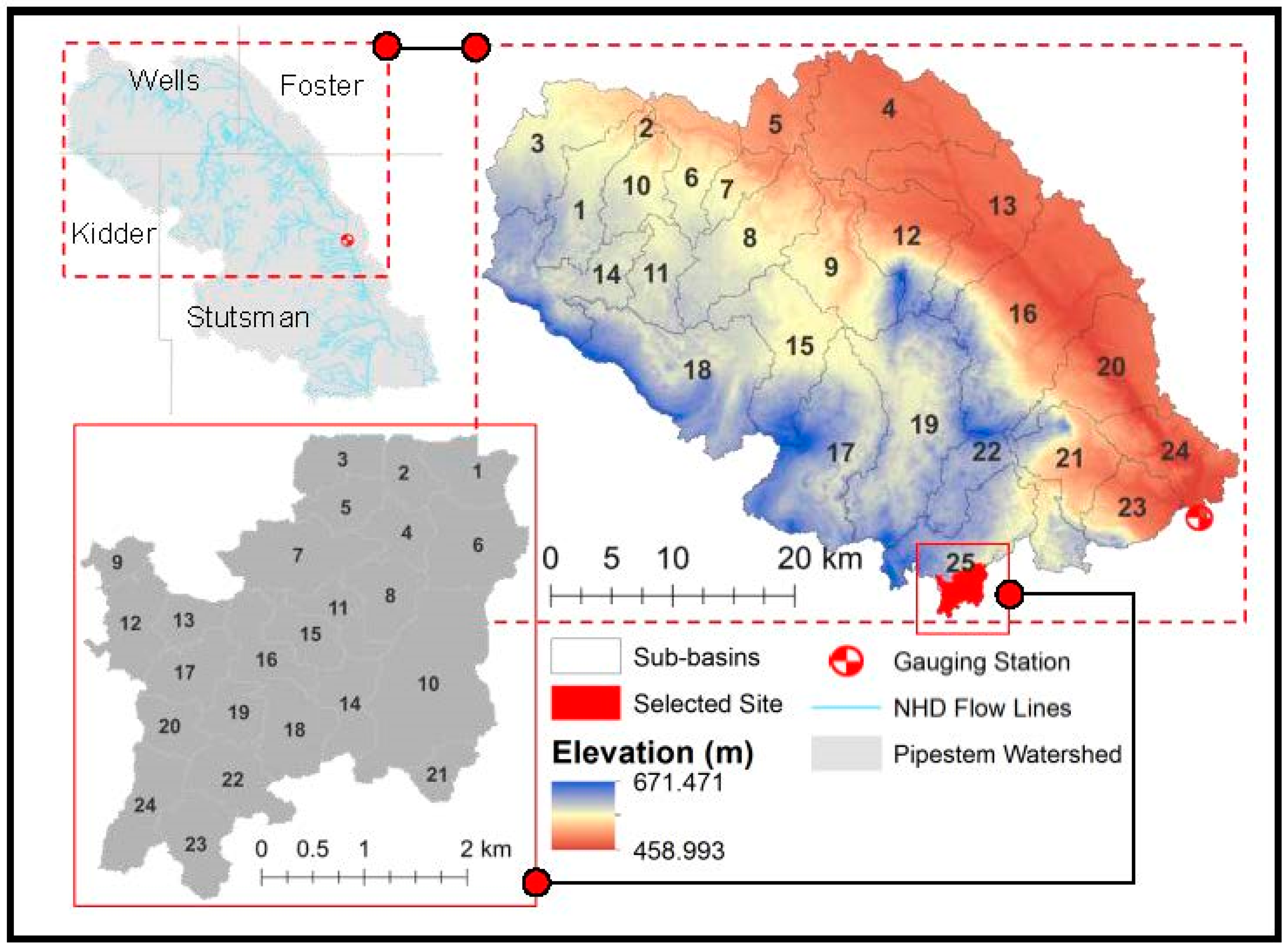
2.3. Testing of the Coupled PD-SWAT Model and Preparation of Input Data

It is aimed in this study to evaluate the coupled PD-SWAT model and emphasize the roles of depressions in the depression-dominated regions. To achieve this goal, a study area within the PPR of North Dakota was selected. Figure 2 depicts the location of the selected area in the Pipestem watershed, which is part of the Missouri River Region and covers parts of four counties including Foster, Kidder, Stutsman, and Wells. Water from the Pipestem watershed drains into the Pipestem Reservoir near the City of Jamestown. The maximum elevation change in the watershed is 47.5 m. According to the National Land Cover Database, the watershed area is mostly covered by herbaceous lands (67.4%). Open water covers 10.5% of the watershed. The Pipestem watershed (2770 km²) consists of five smaller basins or tributaries, including Upper Pipestem Creek, Middle Pipestem Creek, Lower Pipestem Creek, Headwaters Pipestem Creek, and Little Pipestem Creek. The study area was selected with an outlet at the USGS stream gauging station #06469400 at Pipestem Creek NR Pingree (Figure 2). The gauging station has a drainage area of 1813 km² which covers the upper portion of the Pipestem watershed (Figure 2). In addition to this large area, a smaller site (11.4 km², Figure 2) within the boundaries of the larger area was selected to examine the impacts of depression filling-spilling process at an HRU scale.

For the large watershed (Figure 2), both normal SWAT modeling based on the depressionless DEM (i.e., without consideration of depressions) and new coupled PD-SWAT modeling based on the original DEM (i.e., with consideration of depressions) were performed. The simulation results from these two models were compared to analyze the threshold-control functions of depressions and evaluate their impacts on SWAT hydrologic modeling. Eventually, the simulated and observed hydrographs at the outlet of the large area (i.e., USGS gauging station) were compared. The total simulation period was 35 years, ranging from 1974 to 2008. For the purpose of model calibration, the SWAT built-in manual calibration tool was used. First, sensitivity analysis was performed. The t-stat and p-value tests were conducted to identify the significant sensitive and non-sensitive parameters. Then, the ten most streamflow relevant calibration parameters were chosen (

Table 1. Ranking of calibration parameters based on the sensitivity analysis (CN2: runoff curve number, ALPHA_BF: baseflow alpha factor, GW_DELAY: groundwater delay time, GWQMN: threshold depth in the shallow aquifer, GW_REVAP: groundwater revap coefficient, ESCO: soil evaporation compensation factor, SFTMP: snowfall temperature, SOL_AWC: available water capacity of the soil layer, SOL_K: saturated hydraulic conductivity, and SOL_BD: soil bulk density).

Rank	Parameters	Calibration Details			Sensitivity Analysis
		Fitted_Value	Min_Value	Max_Value	t-Stat	p-Value
1	CN2	75.000	40.0	92.0	−25.540	0.000
2	ALPHA_BF	0.369	0.0	0.5	−0.799	0.638
3	GW_DELAY	52.000	30.0	450.0	−2.148	0.033
4	GWQMN	0.785	0.0	2.0	−1.298	0.195
5	GW_REVAP	0.007	0.0	0.2	2.110	0.035
6	ESCO	0.873	0.5	0.9	0.470	0.638
7	SFTMP	−4.925	−5.0	5.0	0.161	0.871
8	SOL_AWC	0.230	0.0	2.0	0.946	0.345
9	SOL_K	4.500	0.0	1500.0	−2.147	0.033
10	SOL_BD	1.250	0.0	10.0	−1.368	0.172

). The ranking of the calibration parameters based on the t-stat and p-value tests is shown in Table 1. Eventually, based on the sensitivity analysis, four parameters, including GW_REVAP, SOL_K, GW_DELAY, and CN2 were found highly sensitive for the model calibration. Therefore, these four parameters were taken into consideration for the final calibration process. Table 1 also shows the minimum, maximum, and fitted values of the calibration parameters. For the small site, the total simulation period was 15 years. Both PD-SWAT and SWAT simulations were performed for two synthetic extreme precipitation scenarios and the dynamic filling-spilling-merging-splitting process of depressions [6] were analyzed.

The observed precipitation data used in this study were obtained from the USDA Agricultural Research Service (USDA-ARS). In addition, the hypothetical precipitation scenarios were generated based on a daily precipitation dataset downloaded for the study area. The first scenario (wet condition) was generated by a 100% increase in precipitation while the second scenario (dry condition) was generated by a 50% reduction in precipitation. The reason for utilizing these synthetic precipitation scenarios is that these extreme precipitation conditions are able to highlight the changes in simulation results from the models with and without considering depressions. The cumulative precipitation in the 156-month simulation period for the wet scenario was about 6 times greater than the one for the dry scenario. To ensure comparable, all other hydrologic and meteorological parameters/data were kept same for the two modeling scenarios. The major meteorological data such as daily minimum and maximum temperatures, daily humidity, daily solar radiation, and daily wind speed were downloaded from the SWAT Global Weather Data portal [26]. Both 30-m and 10-m DEMs of the study area were obtained from the USGS National Map Viewer. Specifically, the 30-m DEM was used for the modeling of the large watershed, and the 10-m DEM was utilized for higher-resolution delineation and modeling of the small site within the large watershed. The land use/land cover and soil type data were obtained from the National Land Cover Database (NLCD 2006), the State Soil Geographic (STATSGO) dataset, and Soil Survey Geographic (SSURGO) database. Particularly, the STATSGO and SSURGO soil data were respectively used for the modeling of the small site and the large watershed.

3. Results

3.1. Depression Characteristics

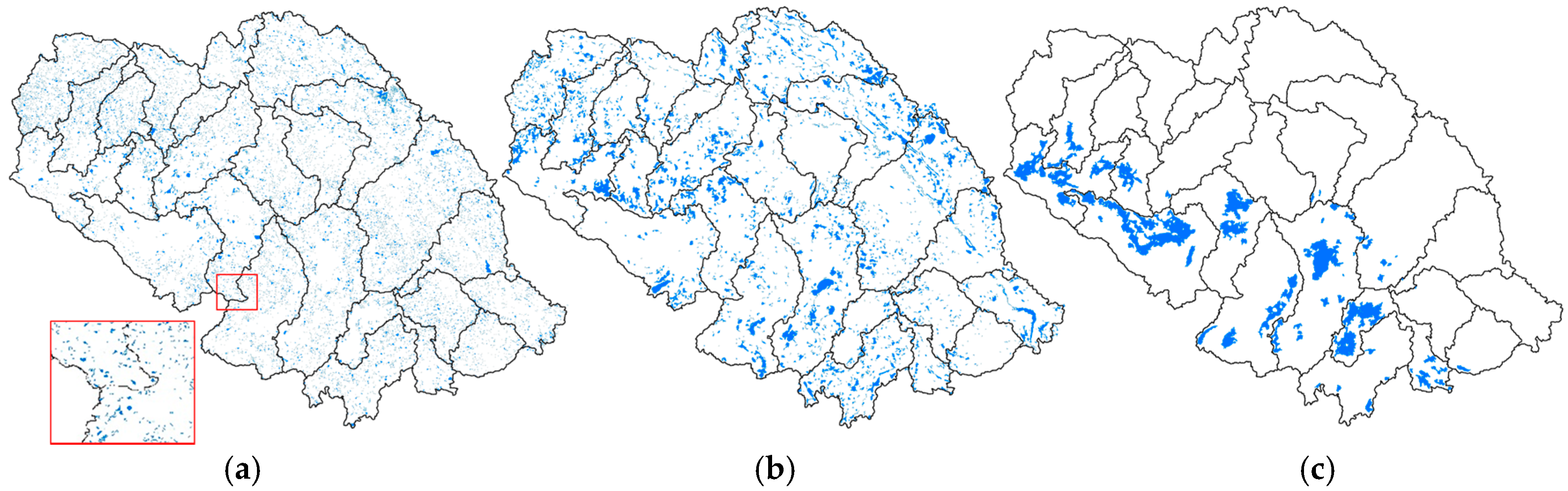
3.1.1. Delineation Results for the Large Watershed

The large watershed was divided into 25 sub-basins (Figure 2) and further subdivided into 505 HRUs. Using the 30-m DEM, PD delineated 18,180 depressions in this large study area. However, a great number of these depressions were one-cell depressions which could be generated by DEM noise. The depression storage of these tiny depressions was close to zero. Based on the mean depth (MD), depressions in the study area were classified into three categories: (1) small depressions: 0 cm ≤ MD < 5 cm; (2) medium depressions: 5 cm ≤ MD < 2 m; and (3) large depressions: MD ≥ 2 m. Figure 3 depicts spatial distributions of the delineated depressions categorized by their mean depths in the large watershed. It can be observed that small and medium puddles (Figure 3a,b, respectively) were almost evenly distributed across the entire study area, while large puddles (Figure 3c) were mostly concentrated on the south-western part of the study area. Out of the 18,180 delineated depressions, 15,939 were identified as small depressions (0 cm ≤ MD < 5 cm), and 6860 of these depressions are one- or two-cell depressions with a mean depth less than 2 cm. Based on these results, it was assumed that these small topographic depressions were artifacts of variations in the DEM. Therefore, all small puddles were excluded in the modeling process. The two remaining categories (medium puddles: 5 cm ≤ MD < 2 m, large puddles: MD ≥ 2 m) were taken into account in the modeling.

Table 2. Characteristics of depressions classified by their mean depths (MD): medium depressions: 5 cm ≤ MD < 2 m and large depressions: MD ≥ 2 m.

Depression Category	Number of Depressions	Sum of Maximum Depression Storages (m3)	Sum of Maximum Ponding Areas (m2)	Mean Depth of Depressions (m)	Storage Capacity of the Largest Depression (m3)
5 cm ≤ MD < 2 m	2170	1.115 × 108	1.268 × 108	0.89	3.1 × 106
MD ≥ 2 m	71	2.764 × 108	7.92 × 107	3.48	5.57 × 107

lists more topographic parameters for these two categories. Table 2 suggests that although the medium depressions cover larger areas than the larger depressions (Figure 3), the capacity of their storages is less than half of the capacity of the larger depressions. In addition, the difference in storage capacity of the largest depressions for these two categories is as high as 5.26 × 10⁷ m³ (Table 2). The largest medium-sized depression can only store 3.1 × 10⁶ m³, whereas the largest large-sized depression can store 18 times more water (5.57 × 10⁷ m³).

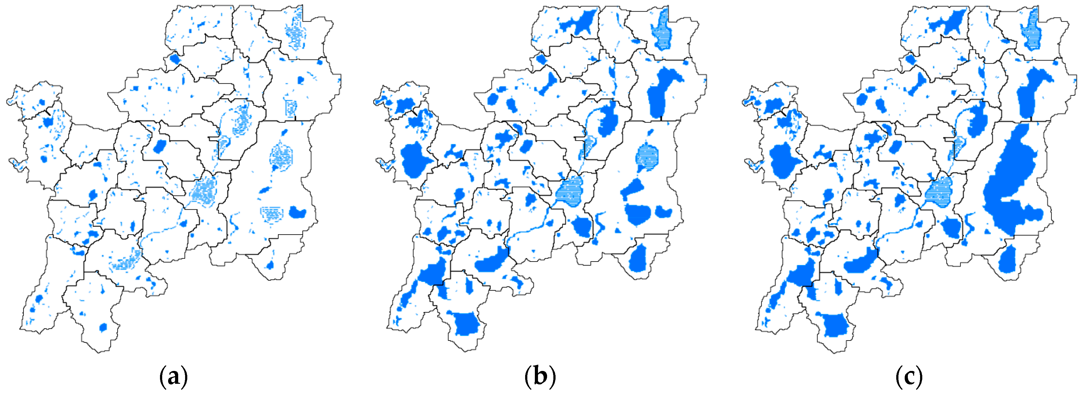
3.1.2. Delineation Results for the Small Site

According to the delineation of the small site from the ArcSWAT modeling system, the small site was divided into 24 sub-basins (Figure 2) and 80 HRUs with unique LULC, soil types, and slopes. The PD program provided details on depression characteristics of this small basin. Total 280 depressions were identified in the 24 sub-basins. The largest and smallest depressional areas were located in sub-basins 10 and 2, covering 594,600 and 10,100 m², respectively. The maximum depression storage (MDS) and maximum ponding area (MPA) of the entire basin were 4,328,733 m³ and 2,109,500 m², respectively.

Table 3. Characteristics of depressions for three selected sub-basins (sub-basins 10, 7, and 2).

Sub-Basin	Sub-Basin Area (m2)	Number of Depressions	Maximum Depression Storage (m3)	Maximum Ponding Area (m2)	Storage Capacity of the Largest Depression (m3)
10	1,647,200	11	2,819,289	594,600	2,814,711
7	784,800	19	37,186	74,000	12,147
2	291,700	12	4195	10,100	4082

summarizes the topographic characteristics of depressions for three representative sub-basins (sub-basins 10, 7, and 2), featuring unique topographic features. Sub-basins 2 and 10 respectively represent two extreme conditions with the minimum and maximum depressional areas, while sub-basin 7 is a typical sub-basin with a moderate number of depressions. As shown in Table 3, sub-basins 10, 7, and 2 contained 11, 19, and 12 depressions with unique storage capacities and ponding areas. The MDS of the largest depression in sub-basin 10 was 2,814,711 m³ (i.e., 65% of the MDS of the entire basin, Table 3).

Figure 4 shows the spatial distributions and hierarchical connections of puddles for three selected puddle levels: level 1 (first puddle level), level 50; and level 243 (final highest puddle level). At the initial level, numerous small puddles were scattered over the surface (Figure 4a). The total number of the first-level puddles was 1186. At level 50, many small puddles merged and the total number of puddles reduced to 289 (Figure 4b). The filling-spilling-merging process [6] continued until all puddles reached their MDS values (Figure 4c), resulting in 280 highest-level puddles. Such a hierarchical structure of puddles and their relationships form a cascaded drainage network that can be used for modeling of the dynamic filling, spilling, merging, and splitting of depressions. Note that the SWAT modeling system (including the ArcSWAT graphical user interface) currently does not have the capability of using all these hydrotopographic details associated with depressions for hydrologic modeling.

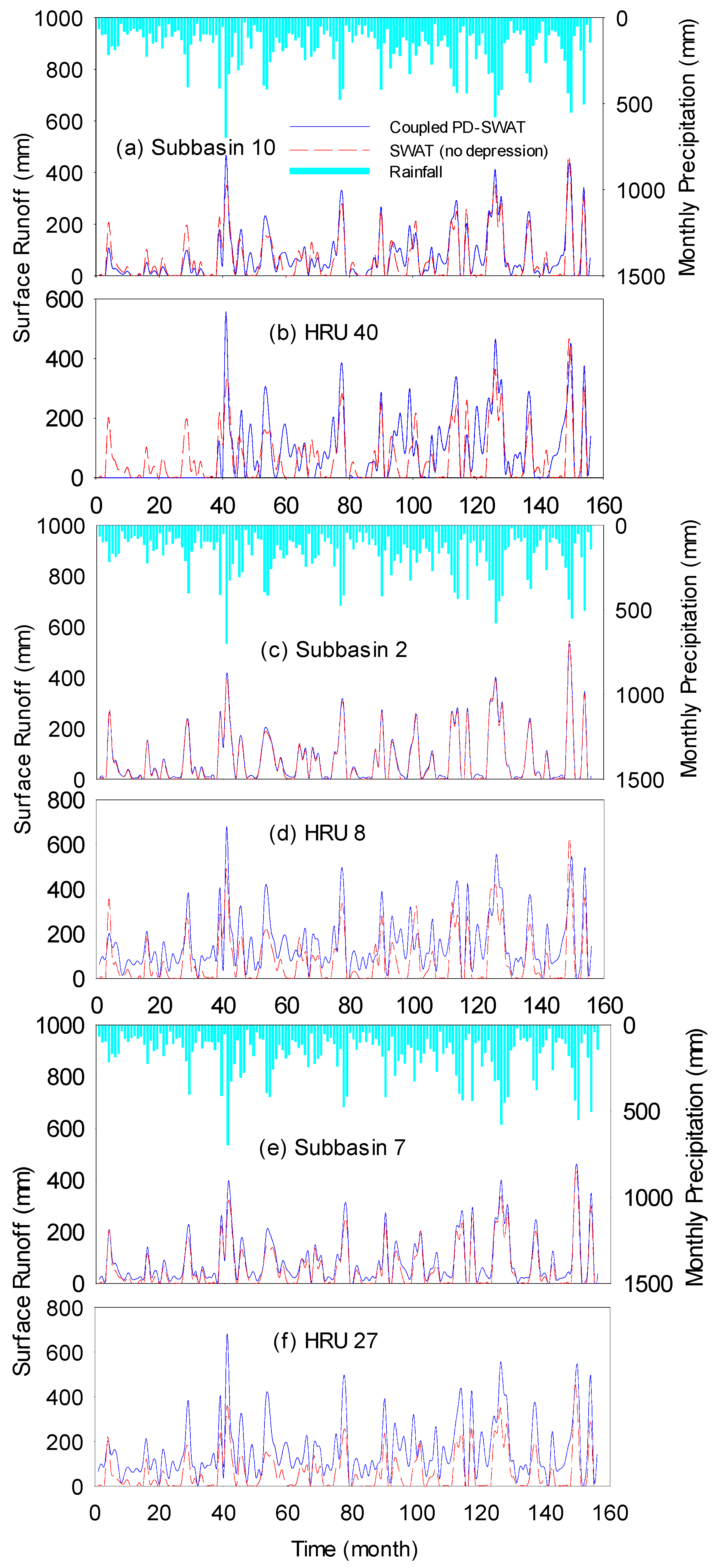
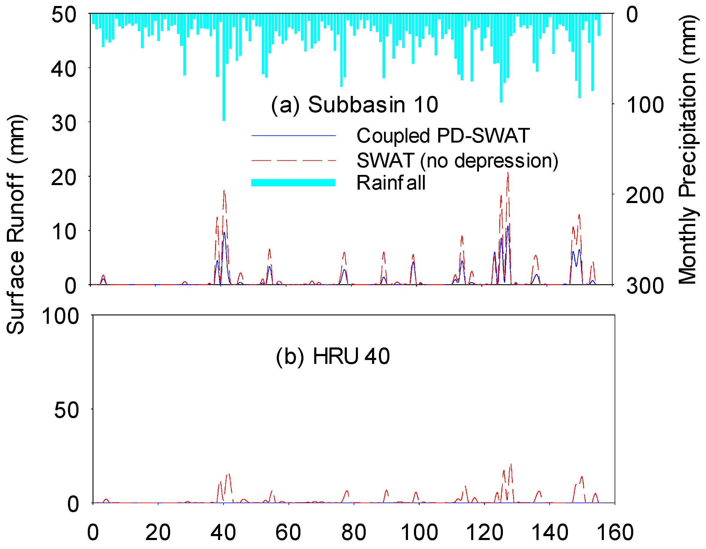
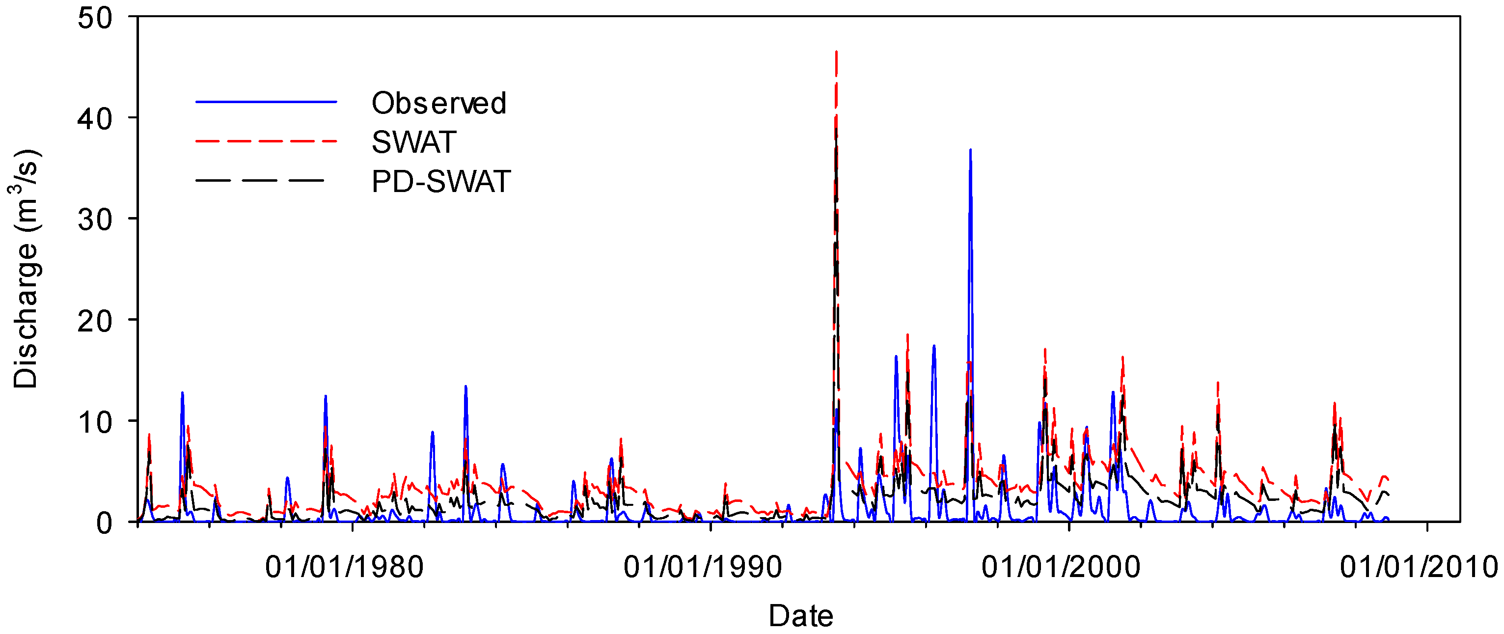
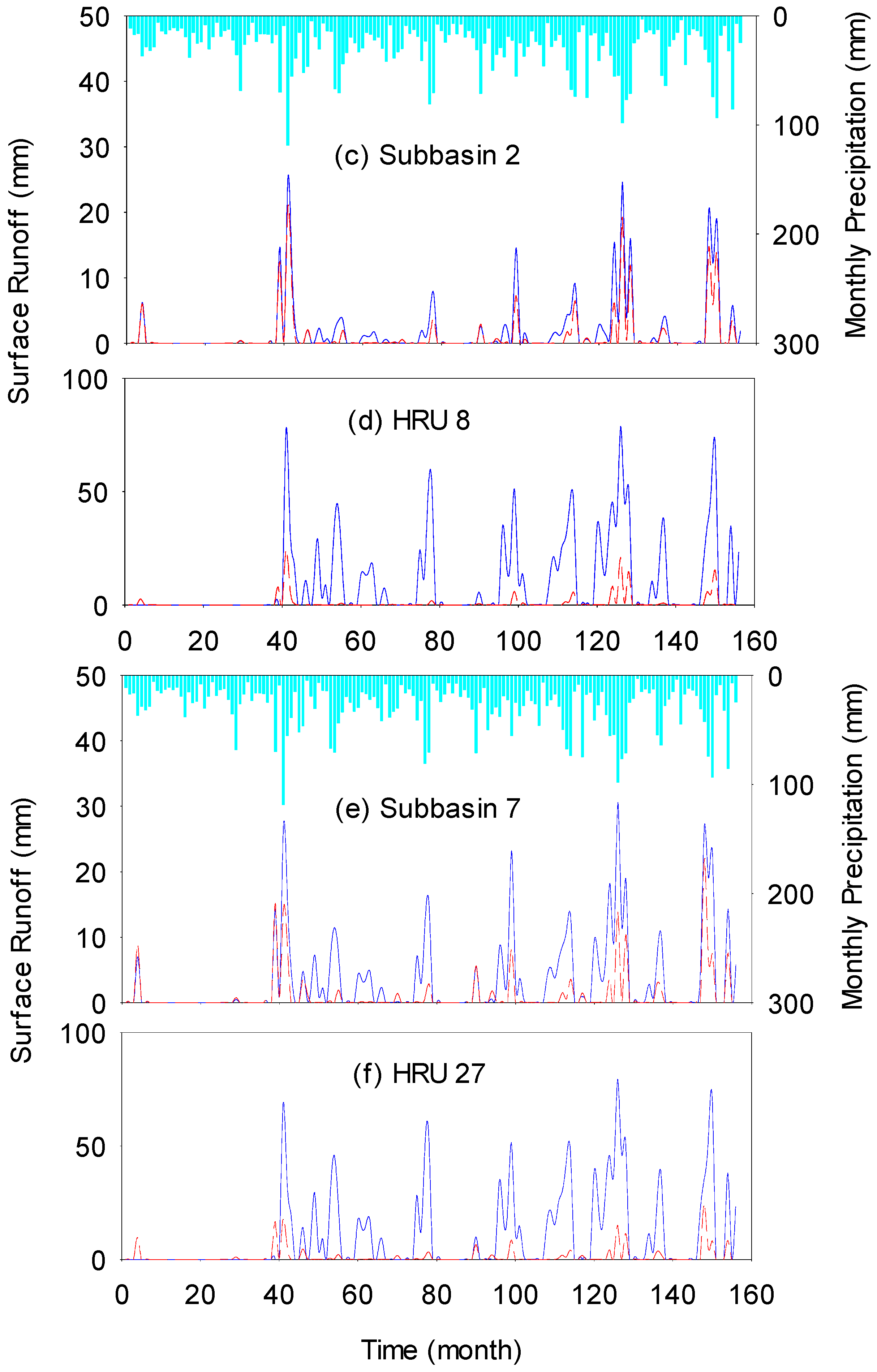
3.2. Threshold-Control Function of Depressions: Depressions as Gatekeepers

Figure 5 compares the hydrographs simulated by SWAT and PD-SWAT against the observed discharge at the outlet of the large watershed. It can be observed that the normal SWAT model consistently overestimated discharges, which can be attributed to its failure to account for the hydrologic effects of surface depressions. This highlights the importance of incorporating puddles and their filling-spilling-merging dynamics into the modeling. Specifically, the modeling results indicated that the effect of puddle incorporation can be directly reflected in the simulated hydrographs. Comparisons of the simulated and observed discharges revealed that PD-SWAT did provide better simulations than the original SWAT.

For the small site, the impacts of depressions on hydrologic modeling were evaluated by examining (1) the differences in surface runoff simulated by the coupled PD-SWAT model and the normal SWAT model; and (2) contribution timing of surface runoff from depressions. Figure 6 shows the comparison of surface runoff simulated by PD-SWAT and SWAT for the three selected sub-basins (sub-basins 2, 7, and 10) and their typical HRUs with depressions/potholes under the extreme high precipitation (Scenario 1). For sub-basin 10, surface runoff simulated by PD-SWAT was much lower than the one from the depressionless DEM-based SWAT model before t = 39 month. When all depressions in sub-basin 10 became fully filled, depression storage reached the MDS (2,819,289 m³), and the depression-dominated HRU of sub-basin 10 (HRU 40) started to contribute runoff to the sub-basin (Figure 6a).

Comparison of the surface runoff simulated by PD-SWAT and SWAT for the depressional HRU 40 of sub-basin 10 in Figure 6b highlights the depression-induced threshold behavior and the resulted delay in the timing of runoff contribution. According to the PD-SWAT simulation results, under the extreme high precipitation, surface runoff initiated till the landscape of HRU 40 reached the fully-filled condition at t = 39 month (Figure 6b). In contrast, the depressionless SWAT model yielded surface runoff from the very beginning, depending on the available precipitation (Figure 6b). After the fully filled time (t = 39 month), the PD-SWAT model with consideration of depressions mostly yielded higher runoff peaks (Figure 6a,b). For example, at t = 41 month surface runoff from PD-SWAT was 463.8 mm, which was 37% higher than the runoff amount (337.2 mm) simulated by the depressionless SWAT model (Figure 6a).

Unlike sub-basin 10, sub-basin 2 had completely different depression characteristics, featuring very limited depressions in terms of both storage and ponding area. Thus, it displayed minimal effects of topographic depressions (e.g., threshold behavior). Resultantly, the surface runoff curves of sub-basin 2 simulated by the coupled PD-SWAT model and the depressionless SWAT model were very similar at the sub-basin scale (Figure 6c). At the HRU scale, however, differences in the simulated runoff can be observed, as shown in Figure 6d for the depression-dominated HRU of sub-basin 2 (HRU 8). Because of small depression storage capacity (4195 m³) in this sub-basin, depressions were quickly filled and HRU 8 started to contribute runoff to the sub-basin from the beginning of the simulation (Figure 6d).

Sub-basin 7 had average topographic characteristics (e.g., number and size of depressions/potholes, MDS, and MPA) (Table 3), and hence the surface runoff curves from both PD-SWAT and the depressionless SWAT model for sub-basin 7 and its depression-dominated HRU (HRU 27) exhibited certain variation patterns between the ones of sub-basins 10 and 2 (Figure 6e,f). As shown in Figure 6f, although depressions were fully filled from the beginning of the simulation, there were notable differences in surface runoff contribution between PD-SWAT and the depressionless SWAT model, which can be attributed to the impact of depression storage of HRU 27. In summary, the similarity and differences in surface runoff for the three selected sub-basins (sub-basins 10, 2, and 7) simulated by PD-SWAT and the depressionless DEM-based SWAT model for this high precipitation scenario demonstrate that the new coupled PD-SWAT model is able to provide improved hydrologic modeling by incorporating simulation of the influences of topographic depressions.

Figure 7 further elucidates the threshold-control function of depressions for the extreme low precipitation scenario. The results for sub-basin 10 (Figure 7a) revealed that surface runoff contribution from the coupled PD-SWAT model was less than that from the depressionless SWAT for the entire simulation period. As shown in Figure 7b, the depression-dominated HRU (HRU 40) did not make any runoff contribution in the PD-SWAT modeling since the low precipitation was not able to fully fill the depressions. However, the cumulative surface runoff simulated by the depressionless SWAT model was 196.5 mm during the simulation period. For sub-basin 2 with minimal depressions, similar to the high precipitation scenario, surface runoff simulated by PD-SWAT and the depressionless SWAT model for the low precipitation scenario did not show any significant differences (Figure 7c). However, surface runoff quantity and contribution timing were different at the HRU scale. Surface runoff contribution of the depression-dominated HRU 8 started at t = 4 month for the depressionless SWAT model, whereas it commenced at t = 39 month in the coupled PD-SWAT modeling (Figure 7d). After this initiation time, PD-SWAT simulated much higher surface runoff (Figure 7d). For sub-basin 7 (Figure 7e), the amount of surface runoff from the coupled PD-SWAT model was also much higher than that from the depressionless SWAT model (Figure 7e). All depressions in HRU 27 were fully filled at t = 43 month and then surface runoff initiated (Figure 7f).

4. Conclusions

In this study, a coupled PD-SWAT modeling approach was proposed to quantitatively account for the filling-spilling process of depressions and the associated threshold control in a semi-distributed manner in SWAT hydrologic modeling for a large watershed and a small site within it in North Dakota. The detailed topographic characteristics, including depressions and their distribution and hierarchical relationships, were determined by the PD algorithm, and further incorporated in SWAT at the HRU scale. To pinpoint the threshold control functions of depressions, a 35-year real precipitation dataset as well as two extreme synthetic precipitation scenarios were considered. The new PD-SWAT modeling was compared against the normal depressionless DEM-based SWAT modeling. It should be noted that this study focused on the modeling methodology to quantify the influences of surface depressions in SWAT modeling.

The simulation results highlighted the important role of threshold control of depressions in hydrologic modeling. Comparisons of the observed and simulated hydrographs at the outlet of the large watershed suggested that the original SWAT model tended to overestimate surface runoff because it was based on dimensionless DEMs and did not account for the effects of surface depressions. According to the PD-SWAT simulations, a depression-dominated HRU started to contribute surface runoff only when all depressions were fully filled. In other words, depressions acted like gatekeepers to control the timing of release of surface runoff. However, it should be mentioned that neither the original SWAT nor PD-SWAT were able to fully simulate the cascaded P2P filling, spilling, merging, and splitting dynamics, as well as the associated hierarchical relationships and threshold control of depressions across different puddle levels and scales. As one of our future efforts to achieve such a modeling goal, the P2P modeling system [6,27] can be integrated with SWAT at certain spatial and temporal scales.

References

1. Euliss, N.H., Jr.; Mushet, D.M.; Wrubleski, D.A. Invertebrates in Freshwater Wetlands of North America: Ecology and Management. In Wetlands of the Prairie Pothole Region: Invertebrate Species Composition, Ecology, and Management; Batzer, D.P., Rader, R.B., Wissinger, S.A., Eds.; John Wiley and Sons: New York, NY, USA, 1999; pp. 471–514. [Google Scholar]
2. Mekonnen, B.; Mazurek, K.; Putz, G. Sediment Export Modeling in Cold-Climate Prairie Watersheds. J. Hydrol. Eng. 2016, 21, 05016005. [Google Scholar] [CrossRef]
3. Ullah, W.; Dickinson, W.T. Quantitative description of depression storage using a digital surface model. II Characteristics of surface depressions. J. Hydrol. 1979, 42, 77–90. [Google Scholar] [CrossRef]
4. Abedini, M.J. On Depression Storage, Its Modelling and Scale. Ph.D. Thesis, Department of Water Resources Engineering, University of Guelph, Guelph, ON, Canada, 1998. [Google Scholar]
5. Chu, X.; Zhang, J.; Chi, Y.; Yang, J. An improved method for watershed delineation and computation of surface depression storage. In Watershed Management Conference 2010; Potter, K.W., Frevert, D.K., Eds.; American Society of Civil Engineers (ASCE): Reston, VA, USA, 2010; pp. 1113–1122. [Google Scholar]
6. Chu, X.; Yang, J.; Chi, Y.; Zhang, J. Dynamic puddle delineation and modeling of puddle-to-puddle filling-spilling-merging-splitting overland flow processes. Water Resour. Res. 2013, 49, 3825–3829. [Google Scholar] [CrossRef]
7. Chu, X. Delineation of Pothole-Dominated Wetlands and Modeling of Their Threshold Behaviors. J. Hydrol. Eng. 2015, 22. [Google Scholar] [CrossRef]
8. Mekonnen, B.A.; Mazurek, K.A.; Putz, G. Incorporating landscape depression heterogeneity into the Soil and Water Assessment Tool (SWAT) using a probability distribution. Hydrol. Process. 2016, 30, 2373–2389. [Google Scholar] [CrossRef]
9. Habtezion, N.; Nasab, M.T.; Chu, X. How does DEM resolution affect microtopographic characteristics, hydrologic connectivity, and modeling of hydrologic processes? Hydrol. Process. 2016, 30, 4870–4892. [Google Scholar] [CrossRef]
10. Arnold, J.G.; Allen, P.M.; Bernhardt, G. A comprehensive surface-groundwater flow model. J. Hydrol. 1993, 142, 47–69. [Google Scholar] [CrossRef]
11. Arnold, G.J.; Srinivasan, R.; Muttiah, R.S.; Williams, J.R. Large area hydrologic modeling and assessment Part I: Model development. J. Am. Water Resour. Assoc. 1998, 34, 73–89. [Google Scholar] [CrossRef]
12. Gassman, P.W.; Reyes, M.R.; Green, C.H.; Arnold, J.G. The soil and water assessment tool: Historical development, applications, and future research directions. Trans. ASABE 2007, 50, 1211–1250. [Google Scholar] [CrossRef]
13. Krysanova, V.; Arnold, J.G. Advances in ecohydrological modelling with SWAT—A review. Hydrol. Sci. J. 2008, 53, 939–947. [Google Scholar] [CrossRef]
14. Qiao, L.; Zou, C.B.; Will, R.E.; Stebler, E. Calibration of SWAT model for woody plant encroachment using paired experimental watershed data. J. Hydrol. 2015, 523, 231–239. [Google Scholar] [CrossRef]
15. Soil and Water Assessment Tool (SWAT). Available online: http://swat.tamu.edu/software/arcswat/ (accessed on 8 December 2016).
16. Sophocleous, M.A.; Koelliker, J.K.; Govindaraju, R.S.; Birdie, T.; Ramireddygari, S.R.; Perkins, S.P. Integrated numerical modeling for basin-wide water management: The case of the Rattlesnake Creek basin in south-central Kansas. J. Hydrol. 1999, 214, 179–196. [Google Scholar] [CrossRef]
17. Shrestha, R.R.; Dibike, Y.B.; Prowse, T.D. Modeling climate change impacts on hydrology and nutrient loading in the upper assiniboine catchment. J. Am. Water Resour. Assoc. 2011, 48, 74–89. [Google Scholar] [CrossRef]
18. Yactayo, G.A. Modification of the SWAT Model to Simulate Hydrologic Processes in a Karst-Influenced Watershed. Master’s Thesis, Virginia Polytechnic Institute and State University, Virginia, VA, USA, 2009. [Google Scholar]
19. Environmental Systems Research Institute (ESRI). Arc Hydro Tools—Tutorial, version 2.0; Environmental Systems Research Institute: Redlands, CA, USA, 2011. [Google Scholar]
20. Almendinger, J.E.; Murphy, M.S.; Ulrich, J.S. Use of the soil and water assessment tool to scale sediment delivery from field to watershed in an agricultural landscape with topographic depressions. J. Environ. Qual. 2014, 43, 9–17. [Google Scholar] [CrossRef] [PubMed]
21. Arnold, J.G.; Allen, P.M.; Volk, M.; Williams, J.R.; Bosch, D.D. Assessment of different representations of spatial variability on SWAT model performance. Trans. ASABE 2010, 53, 1433–1443. [Google Scholar] [CrossRef]
22. Evenson, G.R.; Golden, H.E.; Lane, C.R.; D’Amico, E. Geographically isolated wetlands and watershed hydrology: A modified model analysis. J. Hydrol. 2015, 529, 240–256. [Google Scholar] [CrossRef]
23. Neitsch, S.L.; Williams, J.R.; Arnold, J.G.; Kiniry, J.R. Soil and Water Assessment Tool Theoretical Documentation Version 2009; Texas Water Resources Institute: College Station, TX, USA, 2011. [Google Scholar]
24. Du, B.; Arnold, J.G.; Saleh, A.; Jaynes, D.B. Development and application of SWAT to landscapes with tiles and potholes. Trans. ASAE 2005, 48, 1121–1133. [Google Scholar] [CrossRef]
25. Evenson, G.R.; Golden, H.E.; Lane, C.R.; D’Amico, E. An improved representation of geographically isolated wetlands in a watershed-scale hydrologic model. Hydrol. Process. 2016, in press. [Google Scholar]
26. Global Weather Data for SWAT. Available online: http://globalweather.tamu.edu/ (accessed on 8 December 2016).
27. Yang, J.; Chu, X. A new modeling approach for simulating microtopography-dominated, discontinuous overland flow on infiltrating surfaces. Adv. Water Resour. 2015, 78, 80–93. [Google Scholar] [CrossRef]
Figure 1. Fundamental steps of the coupled SWAT and Puddle Delineation (PD) modeling system (MDS: maximum depression storage, MPA: maximum ponding area, and HRU: Hydrologic Response Unit).
Water 09 00058 g001
Figure 2. Location of the study area in the Pipestem watershed in North Dakota and the delineated sub-basins.
Water 09 00058 g002
Figure 3. Spatial distributions of puddles classified based on their mean depths (MD): (a) small depressions: 0 cm ≤ MD < 5 cm; (b) medium depressions: 5 cm ≤ MD < 2 m; and (c) large depressions: MD ≥ 2 m.
Water 09 00058 g003
Figure 4. Spatial distributions and hierarchical relationships of puddles (blue color) delineated by the Puddle Delineation (PD) program for three selected puddle levels (a) level 1 (initial puddle level); (b) level 50; and (c) level 243 (final puddle level).
Water 09 00058 g004
Figure 5. Comparison of observed and simulated hydrographs by SWAT and PD-SWAT for the large watershed.
Water 09 00058 g005
Figure 6. Comparison of surface runoff simulated by the coupled PD-SWAT and SWAT for three selected sub-basins and their typical HRUs with depressions under extreme high precipitation: (a) sub-basin 10 (depression-dominated sub-basin); (b) HRU 40 in sub-basin 10; (c) sub-basin 2 (lowest depression coverage); (d) HRU 8 in sub-basin 2; (e) sub-basin 7; and (f) HRU 27 in sub-basin 7.
Water 09 00058 g006
Figure 7. Comparison of surface runoff simulated by the coupled PD-SWAT and SWAT for three selected sub-basins and their typical HRUs with depressions under extreme low precipitation: (a) sub-basin 10 (depression-dominated sub-basin); (b) HRU 40 in sub-basin 10; (c) sub-basin 2 (lowest depression coverage); (d) HRU 8 in sub-basin 2; (e) sub-basin 7; and (f) HRU 27 in sub-basin 7.
Water 09 00058 g007aWater 09 00058 g007b