Robust Meter Network for Water Distribution Pipe Burst Detection

Abstract

A meter network is a set of meters installed throughout a water distribution system to measure system variables, such as the pipe flow rate and pressure. In the current hyper-connected world, meter networks are being exposed to meter failure conditions, such as malfunction of the meter’s physical system and communication system failure. Therefore, a meter network’s robustness should be secured for reliable provision of informative meter data. This paper introduces a multi-objective optimal meter placement model that maximizes the detection probability, minimizes false alarms, and maximizes the robustness of a meter network given a predefined number of meters. A meter network’s robustness is defined as its ability to consistently provide quality data in the event of meter failure. Based on a single-meter failure simulation, a robustness indicator for the meter network is introduced and maximized as the third objective of the proposed model. The proposed model was applied to the Austin network to determine the independent placement of pipe flow and pressure meters with three or five available meters. The results showed that the proposed model is a useful tool for determining meter locations to secure high detectability and robustness.

1. Introduction

The robustness of a water distribution system (WDS) is defined as its ability to continue to perform with disturbances. Thus, it is considered different from the traditional reliability, which is focused on the success probability of the system performance [1]. A few early works have confirmed the benefit of considering robustness for different WDS design and operational purposes. Jung et al. [1] confirmed that robustness-based design reduces the failure severity compared to reliability-based design under disturbance conditions not considered in the design phase. Their following study [2] confirmed that considering a robustness measure in WDS pump scheduling optimization produced a time series of consistent pressures, called smoothed pressures, at the critical node.

A meter network is a set of meters installed throughout a WDS that measures system variables, such as the pipe flow rate and pressure. Information is inferred from the meter data for various operational and management purposes. In the current hyper-connected world, meter networks are exposed to meter failure conditions, including malfunction of the meter’s physical system and communication system failure. Cyberattacks are now a major reason for meter failure [3,4]. Therefore, a meter network’s robustness should be secured for reliable provision of informative meter data. In this study, the robustness of a meter network was defined as its ability to consistently provide quality data even under such meter failure conditions.

A meter network’s robustness should be considered in the meter layout phase because the information gain varies for different locations, and the effectiveness of the system output data measured at meter locations should be considered as a whole. Information gains from data collected at some locations can compensate for those at other locations.

In the last two decades, optimal meter placement (OMP) problems have been formulated in order to place meters at their best locations. However, previous OMP studies devoted little effort to considering the meter network’s robustness, even though OMP problems have been considered for various purposes: system state estimation and forecasting [5,6,7], system model calibration [8,9,10], and anomaly detection [11,12,13,14,15]. It has commonly been assumed that all meters perform without any failure, which is not realistic.

This assumption may result in the design of a meter network that is vulnerable to poor performance when the network is partially impaired (e.g., a single meter fails). Especially, more emphasis should be placed on the robustness of a meter network for anomaly detection because a non-robust meter network’s partial meter failure may result in cascading collateral damage. A pipe burst is the rupture of a pipe originating from excessive pressure or ground shifting from temperature changes and earthquakes. Undetected bursts can cause liquefaction of the surrounding soil and sinkholes [15,16]. For example, a meter network for WDS pipe burst detection would have low detectability if a single meter that is designed to detect most of the pipe bursts (i.e., the key player) fails, and the other meters only supplement the key player.

This paper proposes an OMP method for WDS pipe burst detection that considers the robustness of the meter network. A multi-objective OMP (MOMP) model is introduced that maximizes the detection probability (DP), minimizes the rate of false alarms (RF), and maximizes the meter network’s robustness. The meter network’s robustness was quantified through a simulation of single-meter failure. The optimal locations for different types of meters (i.e., pipe flow and pressure meters) were identified independently with a predefined total number of meters (nmeter). The proposed MOMP method was applied to the Austin network. The tradeoff relationships among the multiple objectives and determined meter locations were investigated and compared for the two types of meters.

2. Methodology

This section describes the details of the detection performance measures and meter network’s robustness, the proposed MOMP model, a burst detection method based on the statistical process control (SPC) method, the data generation method, and the optimization algorithm used.

2.1. Detection Performance Measures

Pipes are laid underground; thus, a pipe burst is often not detected until it causes fountaining aboveground or sinkholes. A meter network that can detect many bursts is desired. DP is the proportion of detected burst events to the total number of burst events (nburst). In order to increase the sensitivity of a burst detection method to bursts or increase DP, the control limit beyond which an alarm is issued if the measured value falls should be lowered. However, this can adversely result in an increase in false alarms, i.e., an alarm is issued in response to normal natural random events (under no pipe burst). Therefore, RF, which is the ratio of natural random events for which a false alarm is issued to the total number of natural events (nnormal), is considered along with DP. An optimal meter layout solution would be at the solution point where DP is high before RF begins to significantly increase.

2.2. Meter Network’s Robustness

Based on a single-meter failure simulation, the robustness indicator MeterRob is introduced for a meter network. The simultaneous failure of multiple meters can also be considered, but this is of low likelihood under most accidental failure conditions [4]. In such multiple failure conditions, a WDS manager would want to implement a recovery plan instead of utilizing minimal data received from the impaired meter network. In order to consider the variation in performances of the subsets of a given meter set (robustness), the coefficient of variation (CV) of DP in the event of meter failure is used. MeterRob is calculated as follows.

• Step 1: For a given meter set with a total number of meters N, one of the meters (ith meter, i = 1, ..., N) is assumed to fail in a long time (e.g., for two days). No data measurement is received by the supervisory control and data acquisition (SCADA) system from the meter due to either meter malfunction or communication system failure. Thus, the ith meter’s DP is set to zero.
• Step 2: The network’s DP in the event of failure of the ith meter (DP_f,i) is then calculated.
• Step 3: The failed/impaired meter is then assumed to be back to its normal condition, and another meter is assumed to fail.
• Step 4: Steps 1–3 are repeated until the failure of all meters has been evaluated (i.e., DP_f,i is calculated for i = 1, ..., N).
• Step 5: CV of DP_f,i (CVDP_f) is then calculated:

  $${\mathrm{CVDP}}_f=\frac{\mathsf{\sigma }\left({\mathrm{DP}}_{f,i}\right)}{avg\left({\mathrm{DP}}_{f,i}\right)}, i=1,\dots ,\mathrm{N}$$

  (1)

  where avg(DP_f,i) and σ(DP_f,i) are the average and standard deviation, respectively, of DP_f,i (i = 1, ..., N).
• Step 6: Finally, MeterRob is calculated as:

  $$\mathrm{MeterRob}=1-{\mathrm{CVDP}}_f$$

  (2)

Therefore, a high MeterRob (i.e., MeterRob close to 1) is preferred. This is obtained for a low CVDP_f with low σ(DP_f,i) and high avg(DP_f,i). Note that MeterRob has a value between 0 and 1 because CVDP_f is less than 1. DP_f,i is a ratio value between 0 and 1, so $\mathsf{\sigma }\left({\mathrm{DP}}_{f,i}\right)$ will always be smaller than avg(DP_f,i).

2.3. Multi-Objective Optimal Meter Placement (MOMP) Model

The proposed MOMP model has three objectives: maximize DP (F₁), minimize RF (F₂), and maximize MeterRob (F₃):

$${\mathrm{Maximize}\mathrm{F}}_1=\mathrm{DP},$$

(3)

$${\mathrm{Minimize}\mathrm{F}}_2=\mathrm{RF},$$

(4)

$${\mathrm{Maximize}\mathrm{F}}_3=\mathrm{MeterRob}$$

(5)

The number of meters to be installed is generally determined beforehand by WDS managers considering the available budget [7,17]. Therefore, the number of meters to be installed is predefined as a constraint for the model. The three objective function values are calculated based on the generated control and out-of-control data and the detection and false alarm matrices, which are all described in the following subsections.

Although a few studies have identified a tradeoff relationship between the meter cost and detection effectiveness measure—mostly by using a constrained single-objective model [9,10,17]—DP-type measures (e.g., MeterRob or DP) and RF have not previously been optimized simultaneously. The non-dominated sorting genetic algorithm-II (NSGA-II) [18] was used to explore the tradeoff relationship between the objectives of the MOMP model.

2.4. Pipe Burst Detection Method: Western Electric Company (WEC) Rules

Various data-driven methods have been proposed for WDS pipe burst detection: artificial intelligence [19,20], state estimation [16,21,22], the Bayesian approach [23], classification [24,25], and SPC [15,16,17,26,27,28]. Wu and Liu [29] recently reviewed and classified data-driven approaches; please refer to them for more details of each method. The SPC method identifies any non-random patterns in the measurements of the process variables (e.g., pipe flows and pressures) by utilizing their statistical characteristics obtained from historical measurements under normal conditions. The Shewart control chart is the basis of the SPC method and consists of a centerline representing the time-varying mean value ($\mathsf{\mu }$) of the process variable and warning and control limits (WL and CL, respectively) that are multiples of the standard deviation ($\mathsf{\sigma }$) on each side of the mean value.

Most water utilities monitor the system variables for operational and management purposes at multiple locations. For example, the pressures at the inlet and outlet of each pressure-reducing valve station and the pipe flow at every inlet pipe for a district metering area (DMA) are measured in real-time. These measurements are generally reviewed and analyzed by the system operator/manager and then stored in a database of the water utility. Due to such data availability, SPC methods have been widely applied not only by the WDS research community, but also in practice [15,30].

Jung et al. [15] compared three univariate and three multivariate SPC methods with respect to their DP, RF, and average detection time when provided with common burst data. They confirmed that the Western Electric Company (WEC) rules [31], which are a univariate SPC method, have better detectability than multivariate methods with respect to DP, although the meter locations should be carefully determined because a relatively high RF can occur when more than three meters are used. Univariate methods utilize each process variable’s measurement independently, while multivariate methods consider the correlation between multiple variables under normal conditions [15]. WEC rules are a set of decision rules for identifying non-random patterns in measurements.

In this study, WEC rules were used for pipe burst detection in the MOMP model. The WEC rules raise an alarm if the measurements satisfy any of the following four criteria:

• Rule 1: Any single measurement is beyond the ±4σ CL.
• Rule 2: Two of three consecutive measurements are beyond the ±3σ WL.
• Rule 3: Four of five consecutive measurements are beyond the ±2σ WL.
• Rule 4: Eight consecutive measurements are beyond the ±1σ WL.

Note that Rules 2–4 should be applied to one side of the centerline at a time. Therefore, a measurement followed by a series of measurements on the other side of the centerline outside the WL does not trigger an alarm according to Rules 2–4.

2.5. Data Generation and Detection and False Alarm Matrix

In this study, three sets of pipe flow and pressure data were generated to calculate the objectives of the MOMP model: (1) control data for constructing the Shewart control chart to apply the WEC rules; (2) control data for calculating RF; and (3) out-of-control data for computing DP. The first two datasets were generated by using the hydraulic model of EPANET [32] and entering normal random demands with a diurnal pattern. The out-of-control data were simulated by considering not only normal random demands, but also random pipe bursts with different magnitudes, locations, and initiation times. An emitter in EPANET was used to model a pipe burst whose flow rate (Bflow) is a power function of the burst location’s pressure (p):

$$\mathrm{Bflow}=\mathrm{C}{p}^{\mathsf{\alpha }},$$

(6)

where C is the burst discharge coefficient and α is the power function’s exponent. Uniform random sampling was conducted to select a C value for defining the magnitude of each burst. Two other integer values were sampled for defining the location and initiation time of a burst over the corresponding range (e.g., the range between 1 and the total number of nodes (nn) for determining a burst location when using a pressure meter).

The DP and RF of a given meter set (meterset) were computed based on the detection matrix (D) and false alarm matrix (F), respectively. Each matrix’s elements are binary values (0 or 1) indicating whether an alarm is issued from meter m depending on the n burst/natural event. For example, D_n,m is set to 1 if the mth meter detects the n burst event. The element value of 1 in F indicates a false alarm. To populate the two matrices, the WEC rules were applied to each meter’s data. A number of burst events are considered to have reliable DP and RF values. The matrices D and F are nburst × N and nnormal × N matrices, respectively. Note that N is nn for the pressure meter and np for a pipe flowmeter, where np is the total number of pipes.

A meter configuration matrix (M) is another binary matrix that indicates the location of meters and is an nn × 1 matrix for the pressure meter and np × 1 matrix for the pipe flow meter. A meter is installed at the lth location if M_l = 1 (l = 1, 2, ..., N), and no meter is located there otherwise. Therefore, DP of a given meter set (meterset) is computed as follows:

$${\mathrm{DP}}_{\mathbf{meterset}}={{\displaystyle \sum }}_{m\in \mathrm{meterset}}{{\displaystyle \sum }}_{n=1}^{nburst}\left({\mathrm{D}}_{n,m}\times {\mathrm{M}}_l\right),$$

(7)

where $1\le m\le nn,np$ and $1\le n\le nburst$.

Similarly, RF of meterset is calculated as follows:

$${\mathrm{RF}}_{\mathbf{meterset}}={{\displaystyle \sum }}_{m\in \mathrm{meterset}}{{\displaystyle \sum }}_{n=1}^{nnormal}\left({\mathrm{F}}_{n,m}\times {\mathrm{M}}_l\right),$$

(8)

where $1\le n\le nnormal$.

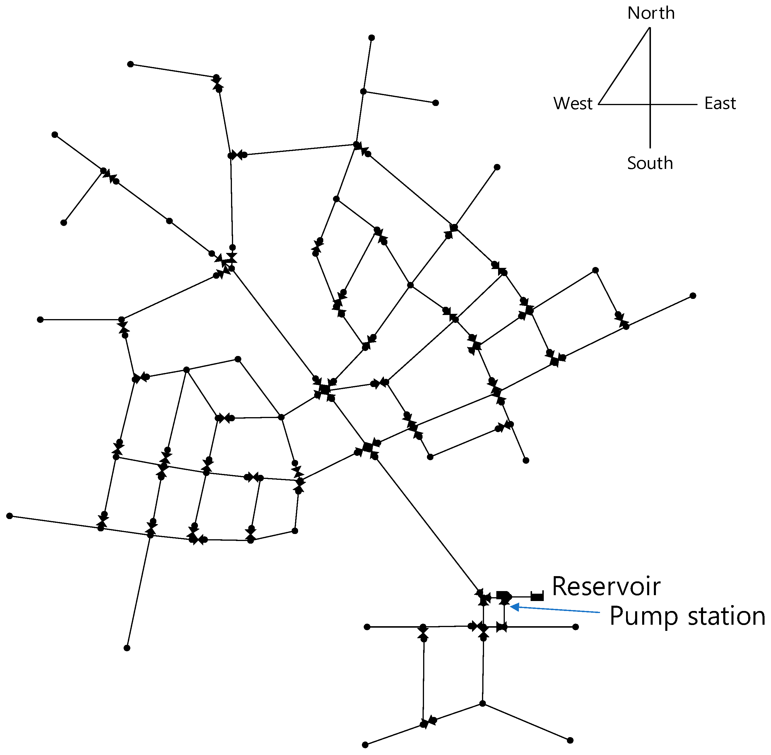
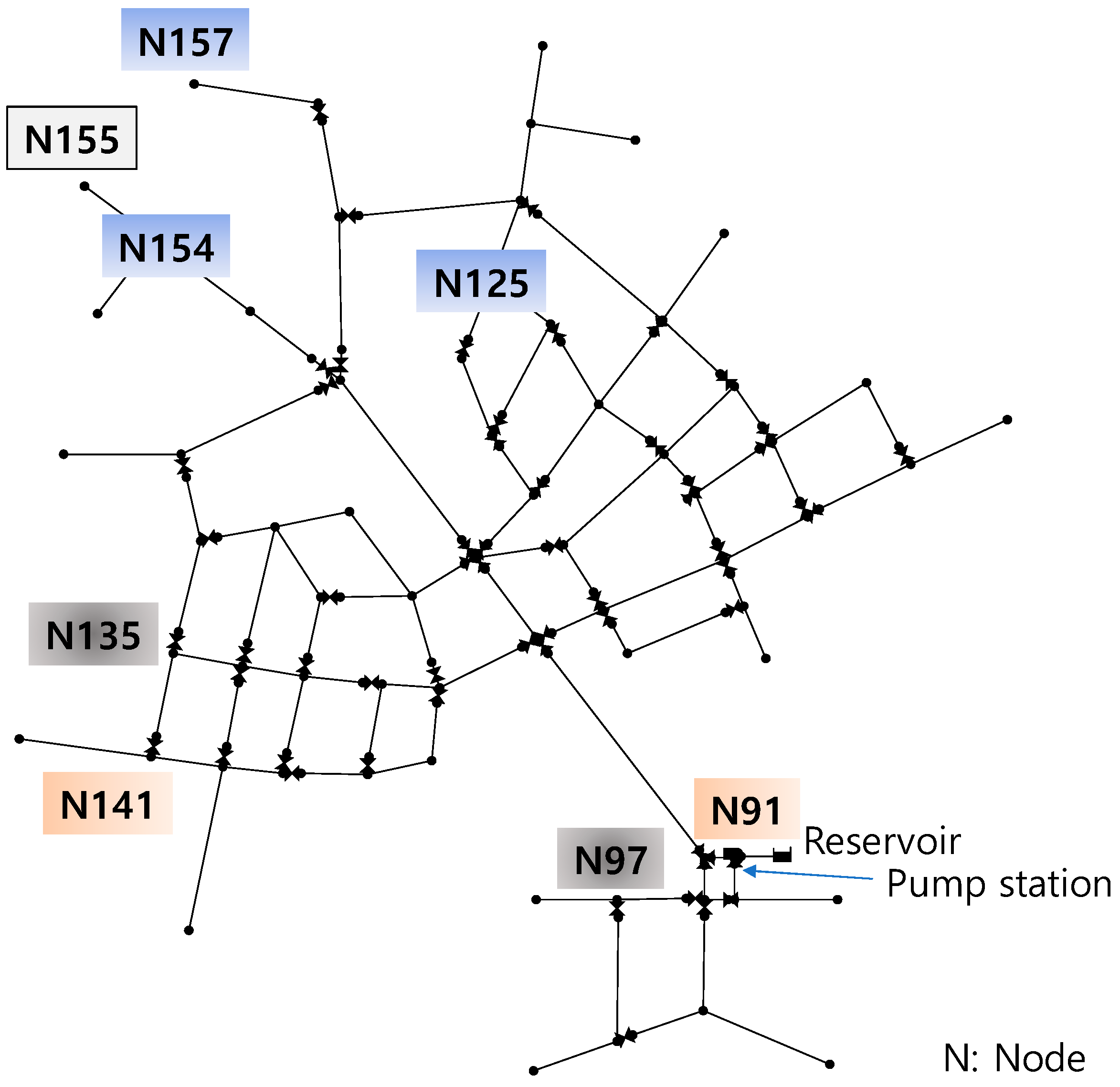
3. Study Network

The proposed MOMP model was applied to the meter placement of a modified Austin network, which has been used for testing SPC methods [15,16] and OMP models for demand estimation [7] and pipe burst detection [17]. The Austin network is a sectionized loop-dominated network with branched pipe lines at the end of the network (Figure 1). The Austin network comprises 90 pipes (np = 90), 126 nodes (nn = 126), one reservoir, and one pump station. The main transmission line is a series of pipes with sizes of 1524, 1219, and 762 mm (60, 48, and 30 in, respectively) passing through the center of the network from the southeast to the northwest mainly to supply the northeastern and southwestern residential areas. Note that industrial customers are in the south-end section, and commercial users are in the north-end section [16]. The total system demand is 726 L/s.

A normal 2000-day series of nodal pressure and pipe flow rates at 5-min time steps was generated to construct the Shewart control chart for applying the WEC rules. The nodal demands were assumed to follow a Gaussian distribution with CV = 0.1 and have a strong temporal correlation with the considered diurnal pattern. Then, 1000 burst events and 1000 natural random events were generated to populate the detection and false alarm matrices, respectively. Only randomness in the nodal demands was considered in the latter, whereas pipe bursts were also simulated to generate the former. For each burst event, three random integer values representing the burst’s magnitude, initiation time, and location were generated. The emitter coefficient C was uniformly sampled over the range of 1 and 100, while the burst initiation time was sampled over the range of 1 and 288 (=24 h × 60 min/5 min), and the burst location was sampled between 1 and nn. The burst magnitudes considered were equal to 0.1–7% of the total system mean demand. Note that the burst flow was modeled by Equation (6) with α of 0.5 in EPANET. A burst that was not detected within 48 h of its initiation was assumed to be a non-detected event. It was also assumed that only a single burst occurred within 48 h.

Starting with randomly generated initial solutions, a population of 200 was evolved over 30,000 generations to yield the final Pareto solution of NSGA-II. Each solution was a string of integer values between the range of 1 and nn for pressure meters and 1 and np for the pipe flow meters to indicate their locations.

4. Results

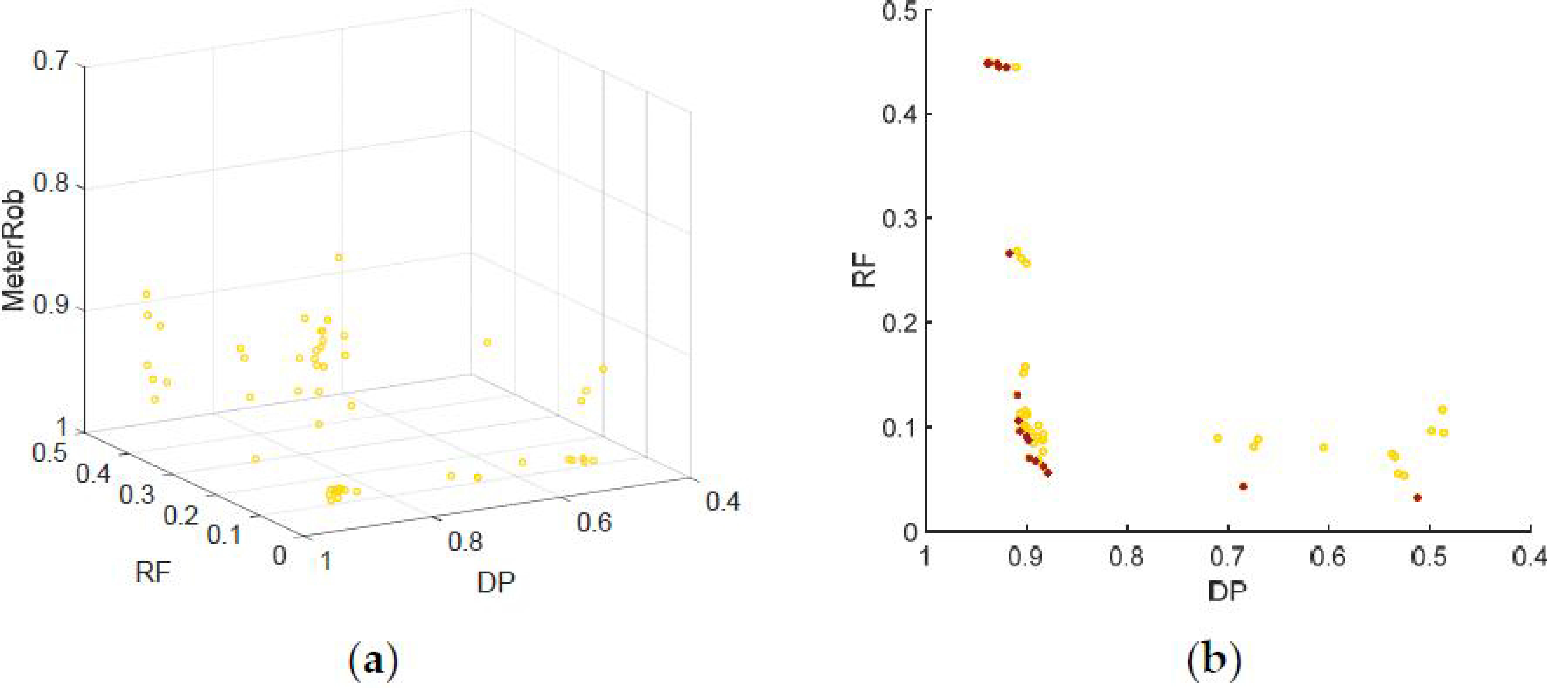
4.1. Pareto Optimal Solutions for Pipe Flow Meter Placement

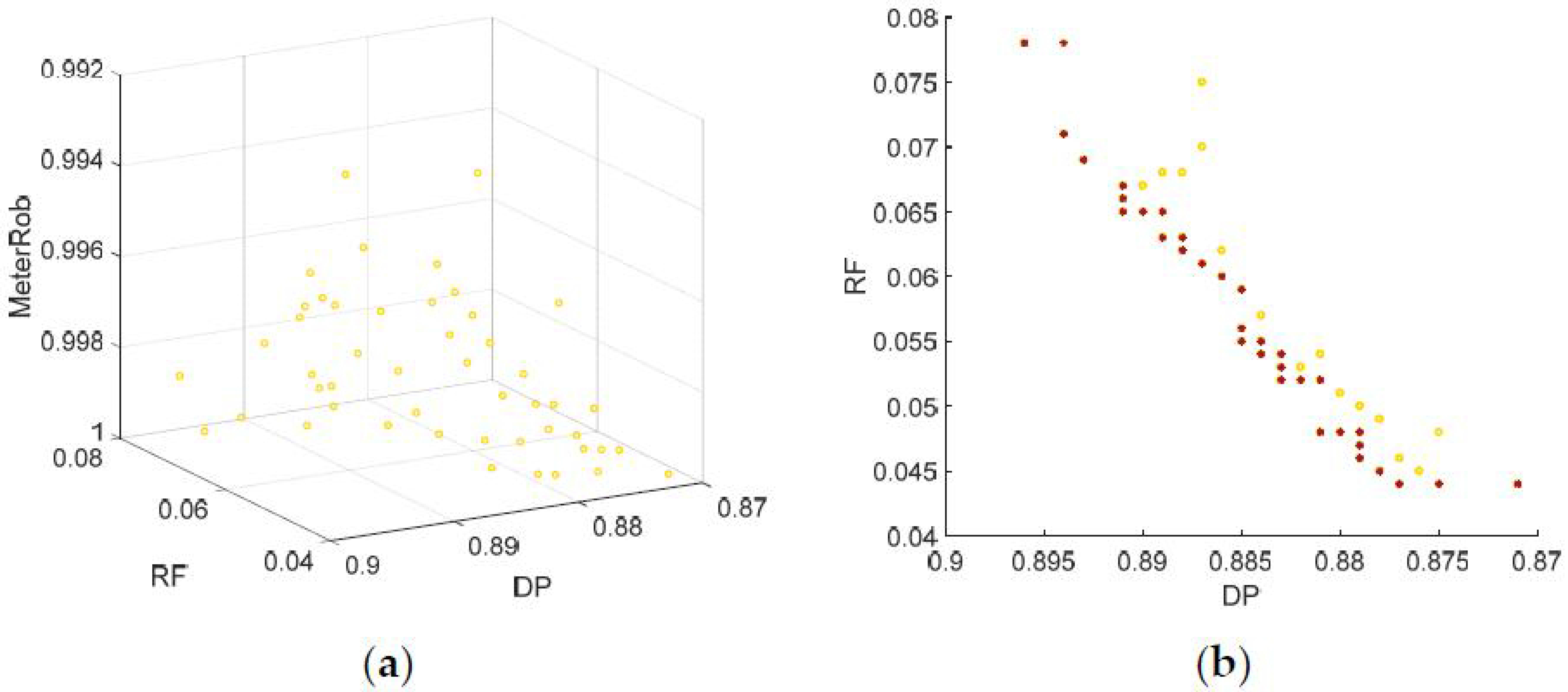
First, the proposed MOMP model was used to determine the location of each type of meter (i.e., pipe flow and pressure meters). The two meter types were independently set to nmeter = 3. The number of available meters was chosen to have sufficient DP and acceptable RF in reference to [15] where the meter locations were determined by engineering sense (e.g., a meter on the main transmission line). Figure 2 shows the projection of the final Pareto optimal solutions in a three-dimensional plot (Figure 2a) and two-dimensional plots of each two-objective set of the three objectives (Figure 2b–d). Each axis was scaled to position the utopian point of (DP, RF, MeterRob) = (1, 0, 1) at the front-most corner of Figure 2a and the lower-left corner of Figure 2b–d. Non-dominated solutions with respect to each two objectives were identified as a post-optimization process and marked with asterisk points in Figure 2b–d.

While the spatial distribution of the Pareto solution points is not easily identified in Figure 2a, the two-dimensional plots provide some interpretation. There exists a nonlinear tradeoff relationship between DP and RF, which indicates that DP can be increased by increasing RF. The marginal increase in RF was significant for solutions with DP > 0.9 (Figure 2b). Therefore, a WDS manager would want to select a solution with DP of around 0.9 and RF of around 0.05 for implementation.

Dominated solutions with respect to DP and RF (circle points in Figure 2b) constituted non-dominated solutions with respect to the other two objectives (i.e., DP and MeterRob in Figure 2c and RF and MeterRob in Figure 2d). For example, the solution of (DP, RF, MeterRob) = (0.883, 0.093, 0.994) is dominated with respect to DP and RF by the asterisk solution of (0.883, 0.062, 0.913) in Figure 2b. However, the former solution is non-dominated with respect to RF and MeterRob in Figure 2d.

MeterRob was confirmed to decrease as DP increased and RF decreased (Figure 2c,d, respectively). This is because (1) pipe flow meters detect different unique bursts, as identified in [17]; and (2) pipe flow meters with relatively high DP generally have high RF. That is, a pipe flow meter sensitive to anomalies tends to be sensitive to natural random events. Therefore, CV of DPs in the event of meter failure increases when high-DP meters are included in the optimal meter sets (i.e., DP increases), which reduces MeterRob (Equation (2)). Again, solutions with DP of around 0.9 and RF of around 0.05 would be preferred by the WDS manager because MeterRob significantly decreases in solutions beyond those values (e.g., a solution with DP > 0.9 in Figure 2c) (Figure 2c,d).

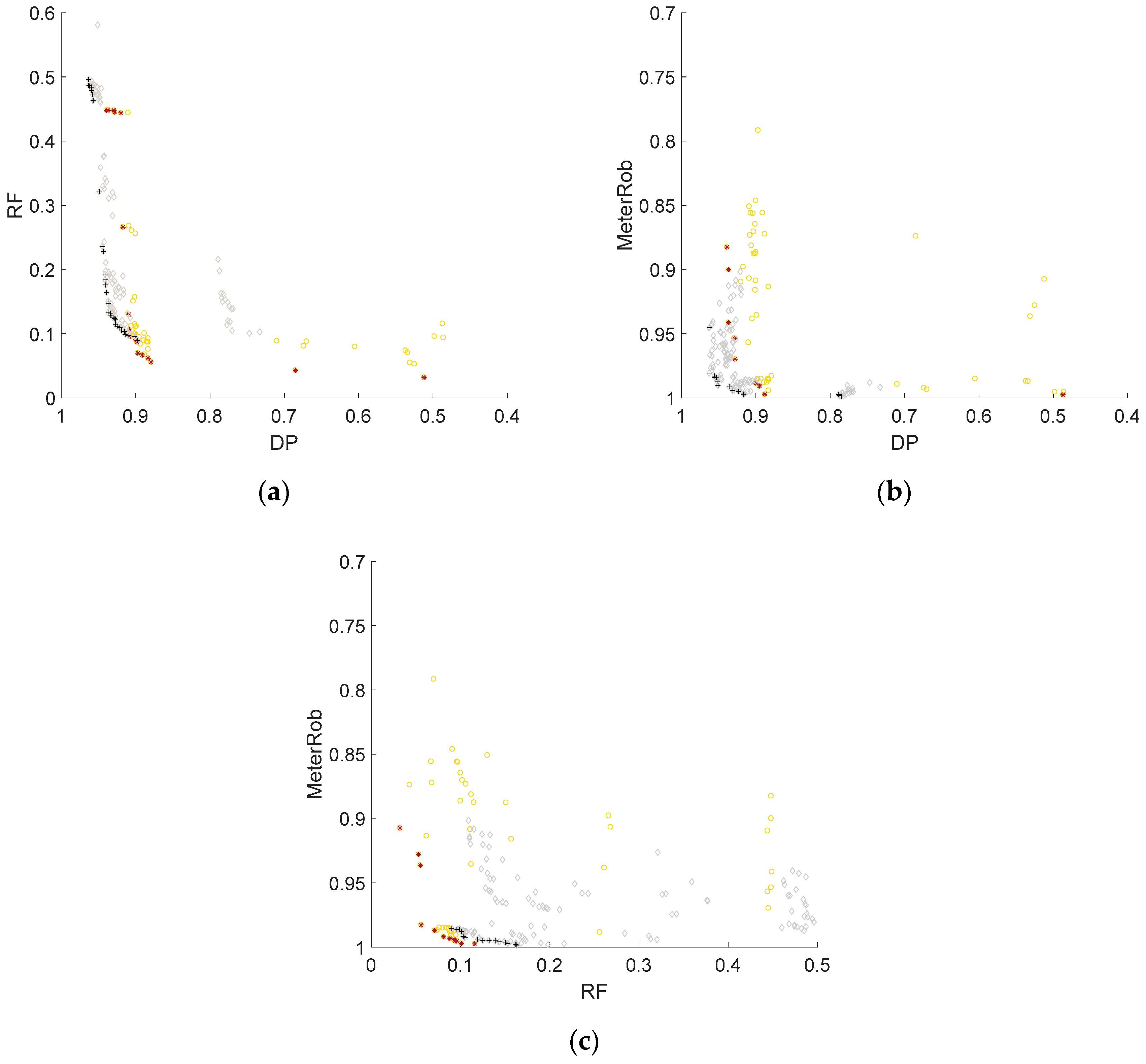
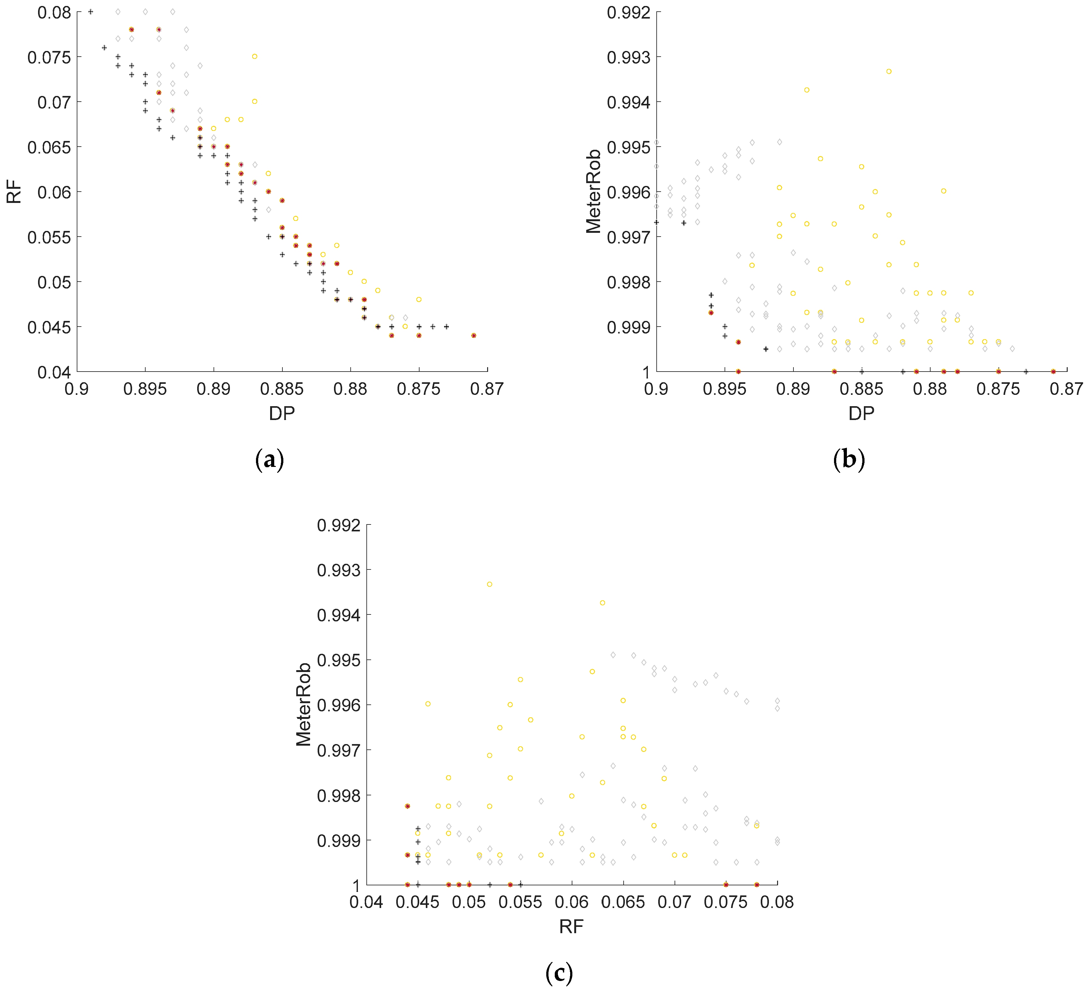
The Pareto optimal pipe flow meter sets were identified for nmeter = 5 using the proposed MOMP model and compared with the solutions obtained for nmeter = 3. Two Pareto solutions were projected onto the two-dimensional plots, where non-dominated solutions with respect to each two objectives were also identified for the Pareto solutions with nmeter = 5 and marked as a cross (Figure 3a–c). When the Pareto frontal solutions in each plot were compared, the solutions for nmeter = 5 were found to dominate those for nmeter = 3 with respect to DP and RF and DP and MeterRob (Figure 3a,b, respectively). That is, the former solutions had a higher DP than the latter solutions for the same or similar RF and MeterRob. Thus, the former’s Pareto front was located to the left side of the latter’s front (Figure 3a,b). This indicates that pipe flow meters issue a false alarm for the same natural random events, while some pipe flow meters are more sensitive to pipe bursts than those at other locations. Therefore, DP can be increased while keeping RF the same for the case of nmeter = 5, which is similar to adding two more pipe flow meters to the case of nmeter = 3. On the other hand, the solutions obtained with nmeter = 5 were dominated by those with nmeter = 3 with respect to RF and MeterRob (Figure 3c).

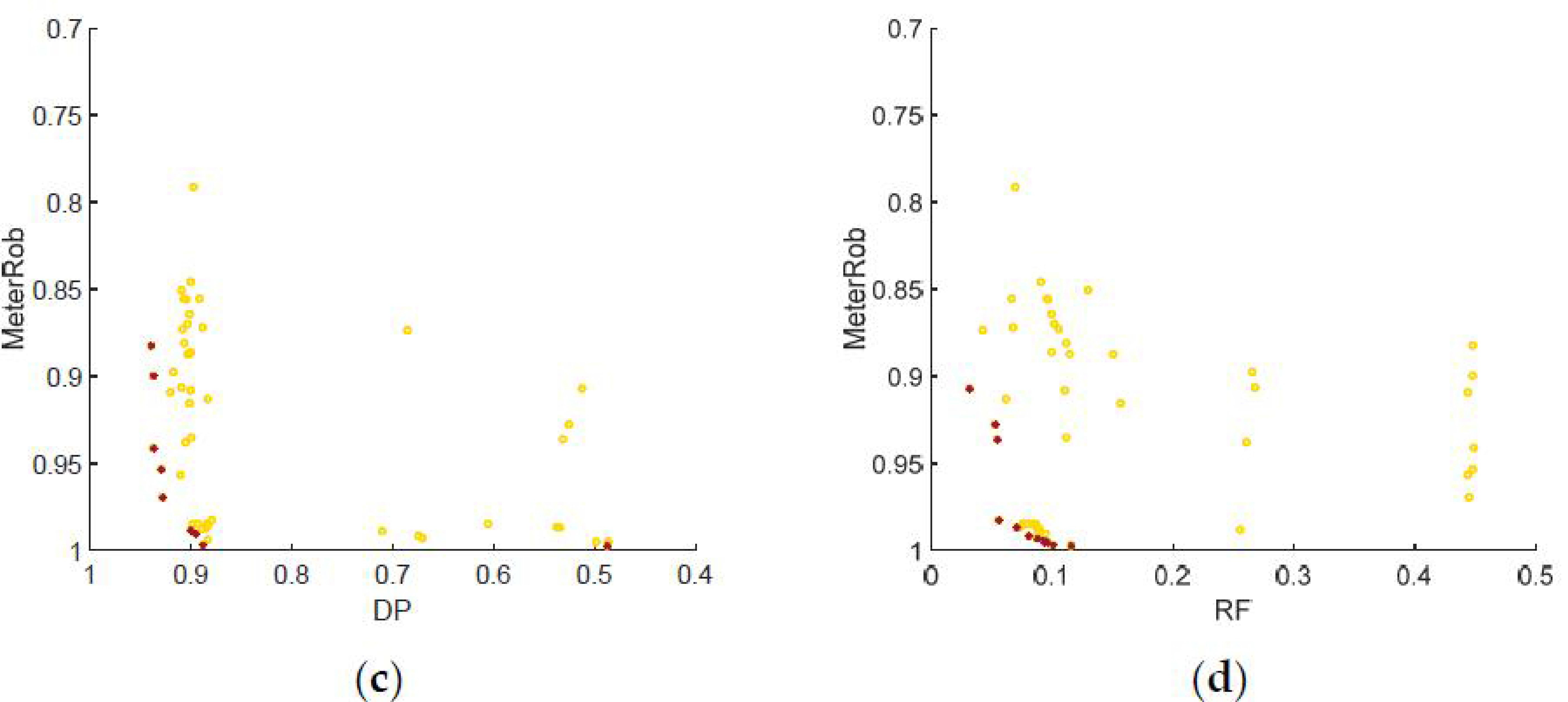
4.2. Pareto Optimal Solutions for Pressure Meter Placement

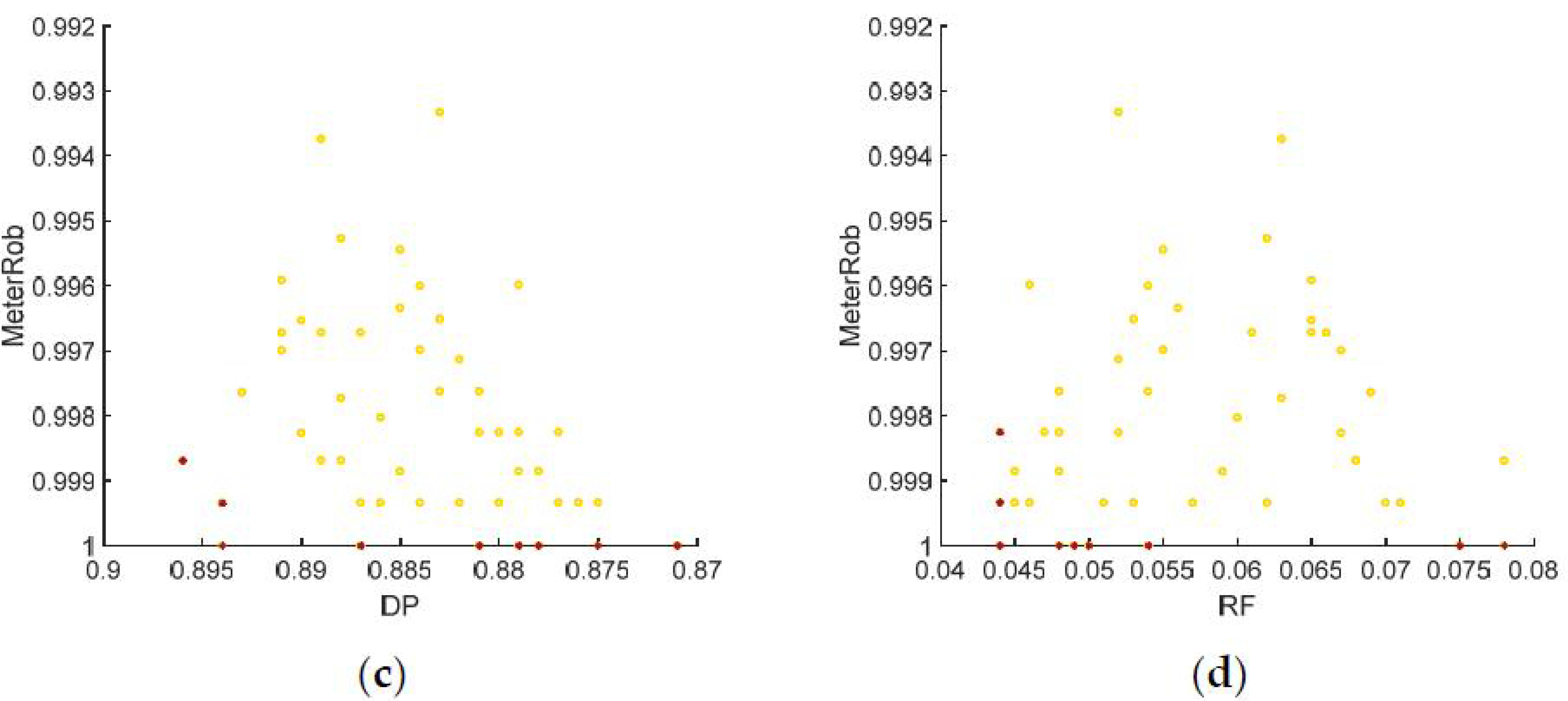
The Pareto optimal meter sets for pressure meter were identified by using the proposed MOMP model given nmeter = 3 and 5. Figure 4 shows the projections of the solutions given nmeter = 3 in a three-dimensional plot (Figure 4a) and two-dimensional plots (Figure 4b–d), similar to that described above. Figure 5 compares the solutions of the two cases for pressure meters in two-dimensional plots.

First, using pressure meters was found to produce higher detectability than using pipe flow meters: DP was between 0.87 and 0.895 and RF was less than 0.08 when three pressure meters were used (Figure 4b). The former ranged between 0.5 and 0.93 and the latter ranged between 0.03 and 0.45 when three pipe flow meters were used (Figure 2b). A linear tradeoff relationship between DP and RF was identified for the pressure meter: the rate of increase for RF was almost the same for all ranges of DP (Figure 4b). In contrast to the pipe flow meter case, the WDS manager would select any solution among the final Pareto optimal sets for the pressure meter case.

Using pressure meters improved the meter network’s robustness more than pipe flow meters. MeterRob was higher than 0.993 for all of the Pareto solutions (Figure 4c), which indicates that an optimal pressure meter set still has high detectability in the event of a single meter failure. Note that MeterRob of the pipe flow meters ranged between 0.8 and 1.0 (Figure 2c). While there was a steep increase in MeterRob for non-dominated asterisk solutions with DP < 0.895, several non-dominated asterisk solutions with MeterRob = 1 existed (Figure 4c). ${\mathrm{CVDP}}_f$ of those solutions was zero because $\sigma \left({\mathrm{DP}}_{f,i}\right)$ = 0, which indicates that the total DPs of the subsets of the optimal meter sets were identical. A sudden increase in MeterRob was also observed around RF = 0.045 for the non-dominated asterisk solutions with respect to RF and MeterRob (Figure 4d).

Therefore, pressure meters should be used for high detectability and robustness of the meter network. In addition, a WDS manager would find it easier to select a solution with pressure meters than with pipe flow meters because the final Pareto solutions of the former had consistent levels of detectability and meter network robustness (i.e., individual meters have similar performance) compared to the latter.

The Pareto optimal solutions of pressure meters given nmeter = 3 and 5 were also compared regarding their non-dominated solution for each two-objective set of the three objectives considered in the MOMP model (Figure 5). Similar to the pipe flow meter case (Figure 3a), the solutions of nmeter = 5 dominated those of nmeter = 3 (Figure 5a). This confirms that pressure meters also tend to issue a false alarm in response to identical natural random events. Therefore, DP can be increased for solutions of nmeter = 5 while maintaining the same or similar RF as solutions of nmeter = 3. Note that the gap between the two Pareto fronts was smaller for pressure meters (Figure 5a) than for pipe flow meters (Figure 3a) because of the consistency in detectability of individual pressure meters.

While apparent non-dominancy between the solutions of the two cases was not observed in Figure 5b, the solutions of nmeter = 3 dominated those of nmeter = 5 with respect to RF and MeterRob for pressure meter placement (Figure 5c), similar to pipe flow meters (Figure 3c). However, the gap between the two Pareto fronts was negligible (i.e., difference of about 0.001 in RF).

4.3. Optimal Meter Placement Comparison

Finally, (1) the meter placement strategies adopted for pipe flow and pressure meters, and (2) the changes in the meter placement for the solutions at different points in the Pareto fronts were compared. Three solutions were selected from the non-dominated asterisk solutions (i.e., Pareto front) of nmeter = 3 with respect to DP and RF for the pipe flow (

Table 1. DP, RF, and MeterRob values of the three selected solutions obtained for three pipe flow meter placements (nmeter = 3).

Solution Identifier	Objective Function Values			Meter Locations
	DP	RF	MeterRob	Meter 1	Meter 2	Meter 3
Solution 1	0.9	0.091	0.846	Pipe 1	Pipe 16	Pipe 33
Solution 2	0.9	0.111	0.908	Pipe 1	Pipe 18	Pipe 5
Solution 3	0.9	0.256	0.988	Pipe 1	Pipe 2	Pipe 79

) and pressure meters (

Table 2. DP, RF, and MeterRob values of the three selected solutions for three pressure meter placements (nmeter = 3).

Solution Identifier	Objective Function Values			Meter Locations
	DP	RF	MeterRob	Meter 1	Meter 2	Meter 3
Solution 1	0.875	0.044	0.9993	Node 125	Node 154	Node 157
Solution 2	0.885	0.059	0.9989	Node 97	Node 135	Node 155
Solution 3	0.894	0.071	0.9994	Node 91	Node 141	Node 155

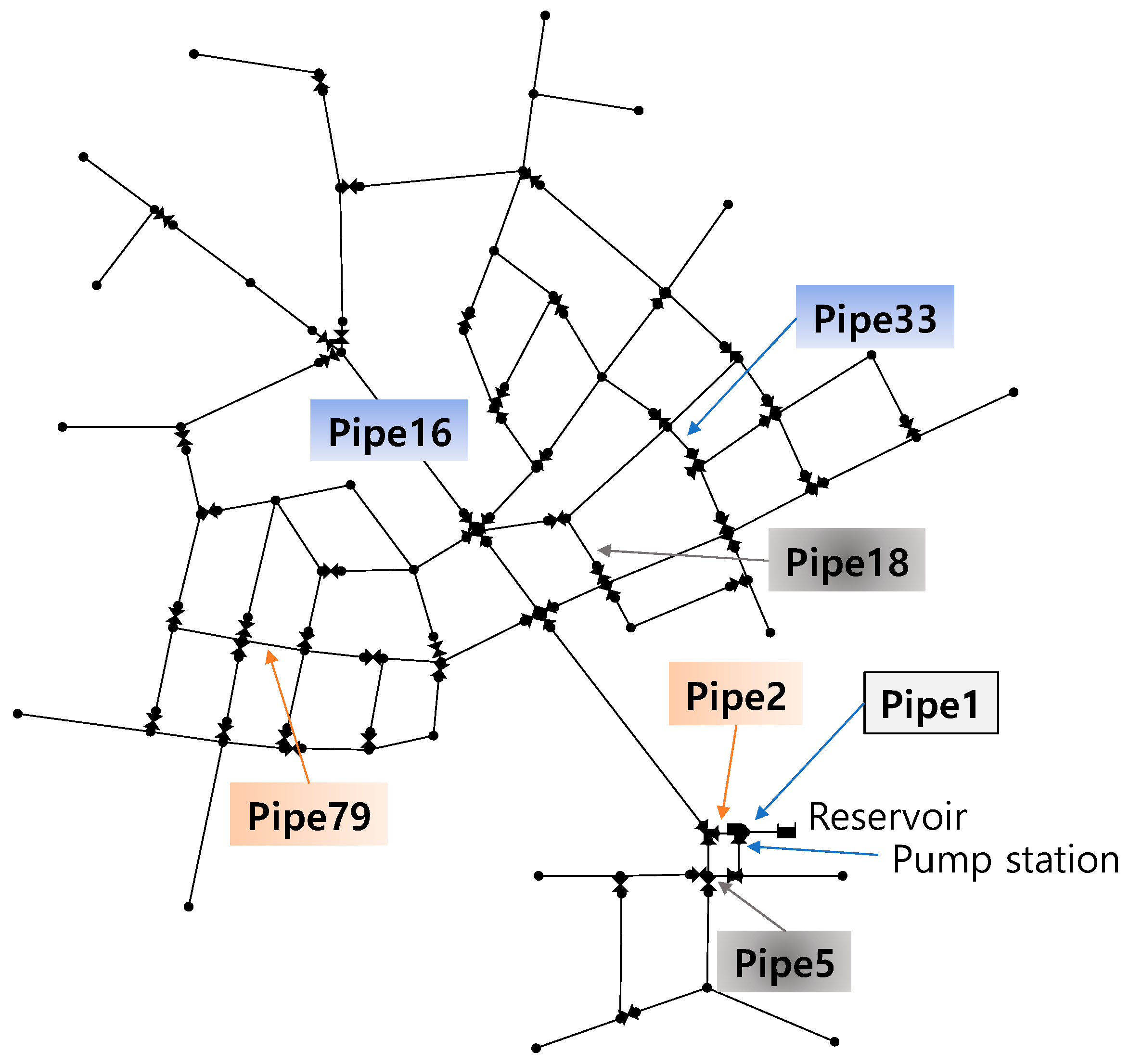
). The selected solutions for the pipe flow meter were on the vertical front shown in Figure 2a where DP = 0.9 (Table 1). On the other hand, the selected solutions for the pressure meter were at each end and in the middle of the linear Pareto front, as shown in Figure 4a (please see their DP and RF values in Table 2). The determined meter layouts of the selected solutions for the pipe flow and pressure meters are shown in Figure 6 and Figure 7, respectively.

While RF and MeterRob increased for the solutions with a higher identifier (i.e., from Solution 1 to Solution 3 in Table 1), a meter was commonly located at Pipe 1 for all three solutions (Table 1). Pipe 1 was a source pipe delivering the total system demand of 726 L/s (Figure 6). The pipe flow contained all nodal demands and, thus, was the most informative and first location to consider when installing a pipe flow meter. For the low-RF and low-MeterRob solution (Solution 1), other meters were located at another transmission pipe with a size of 762 mm (30 in) (Pipe 16) and a local pipe within the northeastern loop (Pipe 33) (Table 1 and Figure 6). RF and MeterRob could be increased by locating the second meter downstream of Pipe 1 at Pipe 2, which also delivered the bulk water demand (Solution 3) (Table 1 and Figure 6). This increased MeterRob by 0.142 (= 0.988 − 0.846) from moving from Solution 1 to Solution 3, although it also caused a significant increase in RF (Table 1).

Both DP and RF increased while MeterRob was maintained (at 0.999) moving from Solution 1 to Solution 3 for the pressure meter (Table 2). Nodes at the end of the network in the north-end section were the most informative location for pipe burst detection; nodes 155 and 157 were common to the three solutions (Table 2 and Figure 7). Pipe bursts occurring throughout the system affected the nodal pressure at the end of the network through increased head losses. Note that a meter was also located at the other end of the network: at node 135 in Solution 2 and node 141 in Solution 3 (Table 2 and Figure 7).

Interestingly, the highest-DP solution (Solution 3) located one meter at Node 91, which was downstream of the source. Therefore, it was found that not only pipe flow meters, but also pressure meters, are placed near the source for high detectability of pipe bursts and high meter network robustness.

5. Summary and Conclusions

This study introduced a MOMP model to maximize DP, minimize RF, and maximize the meter network’s robustness given a predefined number of meters. The meter network’s robustness is defined as its ability to consistently provide quality data in the event of meter failure. Based on a single-meter failure simulation, the robustness indicator MeterRob was introduced and maximized as the third objective of the proposed model. The proposed model was demonstrated on the Austin network for the independent placement of pipe flow and pressure meters. The optimal meter locations were determined for three and five available meters.

The tradeoff relationships of the final Pareto optimal solutions obtained with the proposed model were interpreted according to the non-dominated solutions for each two-objective set among the three objectives DP, RF, and MeterRob. A nonlinear tradeoff relationship between DP and RF was found in the solutions for the pipe flow meter, which indicates that DP is increased by allowing more false alarms. When nmeter = 3, solutions with DP of around 0.9 would be favored by the WDS manager because of the high detection effectiveness and acceptably low RF (i.e., RF around 0.05). MeterRob was found to decrease with increasing DP and decreasing RF because the inclusion of pipe flow meters sensitive to both anomalies and natural random events resulted in a high variation of DP in the event of meter failures.

A linear tradeoff relationship between DP and RF was observed in the final Pareto solutions of the pressure meter for both nmeter = 3 and 5. Using pressure meters was confirmed to increase detectability and MeterRob compared to using the same number of pipe flow meters. While all solutions had MeterRob > 0.993, there were even some solutions with MeterRob = 1 for the pressure meter case in which the total DPs of the subsets of the optimal meter sets were identical. Any solution can be selected in the pressure meter case because of the consistently high detectability and MeterRob. Therefore, pressure meters should be used to ensure not only high detectability, but also meter network robustness.

Regardless of the type of meter, the solutions obtained with nmeter = 5 dominated those with nmeter = 3 with respect to not only DP and RF, but also DP and MeterRob. This indicates that different meters issue a false alarm for the same natural events, which makes it possible to increase DP while maintaining RF when nmeter = 5 compared to when nmeter = 3.

Finally, the optimal meter locations determined by the proposed model given nmeter = 3 were compared in terms of meter placement strategies adopted for different types of meters and for different levels of DP, RF, and MeterRob. The source pipe was confirmed to be the most informative meter location for pipe flow meters, while nodes at the end of the network were the critical locations for pipe burst detection by pressure meters. For the pipe flow meter, the second meter was located at another transmission pipe to increase MeterRob. On the other hand, the second pressure meter was placed at a downstream node of the source for high DP. Regardless of the type of meter, the remaining meter could be installed in a local area, such as within a looped subsection of the network.

The proposed MOMP model was concluded to be a useful tool for determining meter locations that secure high detectability and meter network robustness. The meter network robustness should be considered in meter placement to maintain the network’s performance under failure conditions.

This study had several limitations that future research must address. First, this study focused on introducing and demonstrating the MOMP model and comparing the optimal meter locations determined by different type of meters and given different numbers of available meters. Pipe flow and pressure meters can be simultaneously considered, and the optimal ratio between the two meters can be determined given the number of available meters. Second, this study used two different numbers of meters, as suggested by a previous study. However, a thorough sensitivity analysis can be conducted by using the proposed model with different numbers of meters, for example, with nmeter = 1–10. Finally, multiple simultaneous meter failures can be considered to quantify the meter network’s robustness, especially for a large network with many meters.