Analysis of Current and Future SPEI Droughts in the La Plata Basin Based on Results from the Regional Eta Climate Model

Abstract

We identified and analysed droughts in the La Plata Basin (divided into seven sub-basins) for the current period (1961–2005) and estimated their expected evolution under future climate projections for the periods 2011–2040, 2041–2070, and 2071–2099. Future climate projections were analysed from results of the Eta Regional Climate Model (grid resolution of approximately 10 km) forced by the global climate model HadGEM2-ES over the La Plata basin, and considering a RCP4.5 emission scenario. Within each sub-basin, we particularly focused our drought analyses on croplands and grasslands, due to their economic relevance. The three-month Standardized Precipitation Evapotranspiration Index (SPEI3) was used for drought identification and characterization. Droughts were evaluated in terms of time (percentage of time from the total length of each climate scenario), space (percentage of total area), and severity (SPEI3 values) of cells characterized by cropland and grassland for each sub-basin and climate scenario. Drought-severity–area–frequency curves were developed to quantitatively relate the frequency distribution of drought occurrence to drought severity and area. For the period 2011–2040, droughts dominate the northern sub-basins, whereas alternating wet and short dry periods dominate the southern sub-basins. Wet climate spread from south to north within the La Plata Basin as more distant future scenarios were analysed, due to both a greater number of wet periods and fewer droughts. The area of each sub-basin affected by drought in all climate scenarios was highly varied temporally and spatially. The likelihood of the occurrence of droughts differed significantly between the studied cover types in the Lower Paraguay sub-basin, being higher for cropland than for grassland. Mainly in the Upper Paraguay and in the Upper Paraná basins the climate projections for all scenarios showed an increase of moderate and severe droughts over large regions dedicated to crops and grasses. On the other hand, for the near future, the Lower Uruguay and the River Plata basins showed a decrease of drought severity compared to the current period. Projections suggest an increase in competition among uses in these regions and the need for a potential relocation of certain crops from the northern regions towards cooler regions located in the centre and south. Further research should consider other climate projections and perform high spatial resolution studies in localized areas.

1. Introduction

The La Plata Basin (LPB) is located in the centre-south of South America. It comprises five countries with a total extent of 3,174,229 km². As droughts affect economic and social activities within the basin [1], the study of present and future climate scenarios is essential. In this study, drought is understood as a period which is drier (e.g., resulting from lower rainfall or/and higher temperatures) than usual. Several authors have focused their work on specific drought spells that occurred over certain regions within the La Plata Basin (e.g., [2,3,4,5,6,7]). Comprehensive works on droughts were mostly conducted on monthly time-scales (e.g., [3,8,9,10,11]) and a few on daily time-scales [4,12]. In general, they showed a decrease of drought spells after the mid-1970s. For example, Penalba and Vargas [9] detected a 20% decrease in the number of dry months per year, and Barrucand et al. [3] reported fewer dry months during the warm season (October to March) between 25 °S and 40 °S in the region, passing from 2–3 months during 1904–1920 to 1–2 months from 1980–2000. Moreover, various studies have documented inter-annual trends in the region’s climate over the last 40 years [13]. Doyle et al. [14] described an increase in the annual precipitation in the region by 5 mm/year between 1960 and 2005. Penalba and Robledo [15] reported a 10–25% decrease in daily rainfall in winter, but a 33–60% increase in the remaining seasons during 1950–2000. Dufek et al. [16] reported a 7–9% increase in the number of warm nights and a 5–9% decrease in the number of cold nights in most of the region during 1961–1990. Much literature describes severe droughts in recent years [5,6,12,17,18,19,20].

With regard to the modelling of the current climate and the evaluation of projections of the effects of climate change on the basin, several studies were conducted by assembling different emission scenarios (RCP 8.5, RCP 6.0, RCP 4.5, and RCP 2.6) with regional climate models (RCM, e.g., REGCM3, RegCM4, Eta, RCA, MM5, and REMO) driven by global climate models (GCM, e.g., HadGEM2, HadCM3, MIROC5, EC5OM, ECHAM5, GFDL, and MPI) (e.g., [3,11,13,21,22,23,24,25,26,27,28,29,30,31,32,33,34,35,36,37,38,39,40]). In order to assess a wide range of uncertainty sources, in recent years many studies have followed an ensemble modelling approach. This implies the generation of ensembles of simulations performed with different RCMs driven by different GCMs for different emission scenarios. However, this has prompted debate over both the appropriate interpretation of ensembles as well as how best to communicate uncertainty about future climate change to decision makers [41]. The most ambitious collaborative initiative for producing ensembles of RCM simulations over the La Plata Basin was performed within the CLARIS-LPB Project (a Europe–South America network for climate change assessment and impact studies [42,43]). A suite of seven coordinated RCM simulations over South America (with an approximate grid resolution of 50 km) driven by both the ERA-interim [44] reanalysis and a set of GCMs were evaluated [34,36,37,38,39,40,42]. Carril et al. [36] found relatively good agreement for the annual precipitation average cycle over the La Plata Basin by applying an ensemble of RCMs. Moreover, they stated that these results were due to the cancelation of offsetting errors in the individual models. Menéndez et al. [37] found that the ensemble seasonal (December, January and February, DJF) mean precipitation compared to the CPC-Unified Gauge-Based data [45] is underestimated in the southern LPB down to 3 mm/day and it is overestimated in the northern and eastern LPB up to 4 mm/day. Solman et al. [38] found that although the results of the ensemble of the RCMs systematically improved the quality of the modelled climate compared to the single RCM model evaluated in the CLARIS-LPB project, they did not identify anyone producing systematically worse or better results for every variable over every region. Moreover, they highlighted that the individual models should be built and evaluated after a deep analysis of the characteristics of the study region. In that sense, the National Institute for Space Research (INPE, São Paulo, Brazil) started using and developing different versions of the Eta Model [46,47,48,49,50,51] for regional climate simulations and projections in the region at the beginning of the XXI century and thus has an excellent knowledge of the study region [46,47,48,51,52,53,54,55,56]. Based on previous studies [24,51,52], Mourao [27] applied to the La Plata Basin the Eta Regional Climate Model with a grid resolution of approximately 10 km and forced by the global climate model HadGEM2-ES [57,58,59]. Validation of the model for the current period (1961–1990) was performed based on the Climatic Research Unit database (CRU) [60]. In general, the Eta Model is capable of capturing the spatial and temporal patterns of precipitation and temperature compared to the observed data and precedent studies. In DJF the daily average precipitation is underestimated by 1 mm/day in the north and overestimated by 1 mm/day over the east and south border of the basin. The DJF average temperature is underestimated by 2 °C over the east border of the basin. Under- and over-estimations by about 1 °C are observed in the north of the basin. However, Menéndez et al. [37] found that the ensemble seasonal (DJF) temperature compared to the CRU data [60] is overestimated by 3 °C in the southern and western LPB and underestimated by 2.5 °C in the eastern LPB. In addition, they estimated the potential evapotranspiration (PET) for the current climate.

Concerning the future climate, several models showed, in general, a precipitation increase over the La Plata Basin region [29,30,31,33,34,37]. According to Menéndez et al. [37], for the period 2071–2100, the seasonal mean precipitation (DJF) from the CLARIS LPB ensemble under the SRES A1B scenario is projected to increase between 20% and 40% over the southern LPB. A slight decrease to 5 % or stability of precipitation is projected over the northern LPB. Moderate increases ranging 5–30% are projected over the remaining regions of LPB. Considering an RCP4.5 emission scenario [61] and compared to the 1961–1990 period, Mourao [27] reported that the projection of the daily average precipitation in DJF indicates an increase of up to 1 mm/day in the south and a decrease down to 3 mm/day in the north of the basin for the period 2011–2040; an increase of up to 1 mm/day in the south, southwest and west, and a decrease down to 1 mm/day in the north and northeast of the basin for the period 2041–2070; and an increase in the south/southwest of up to 2 mm/day and a decrease in the north/northeast down to 1 mm/day for the period 2071–2099. On the other hand, most of the RCMs and ensembles agree that the average temperature for the entire trimester (DJF) is projected to increase. Menéndez et al. [37] reported an increase of up to 2 °C over the southern and up to 4 °C over the northern LPB. They also analysed the evapotranspiration projection for the period 1971–2100 (DJF), finding an increase up to 30% between 20° S and 40° S compared to the current climate (1960–1990). Mourao [27] reported the greatest differences of temperature between the 10° S and 23° S latitudes with a DJF average temperature increase of up to 3 °C between 2011 and 2040, 3.5 °C between 2041 and 2070, and 4 °C between 2071 and 2099.

Drought indices are often used to monitor droughts, and the information derived from these indices can be used in planning and designing applications. The World Meteorological Organization (WMO) and the Global Water Partnership (GWP) [62] presented some of the most commonly used drought indices applied across drought-prone regions. They were categorized by type and ease of use, including meteorology, soil moisture, hydrology, remote sensing and modelled indices. The SPI drought index (Standardized Precipitation Index [63]) is widely used worldwide, and it has been applied in LPB [7,9,22,34]. By applying the SPI3 and using a CMIP5 multi-model ensemble, Penalba and Rivera [22] analysed future changes in drought characteristics over southern South America, finding that the occurrence of droughts will be more frequent during the 21st century, with shorter durations and greater severities. The projections show increases in drought frequency changes of about 10–30%, accompanied with increases of 5–15% in the mean drought severity and a decrease of 10–30% in the mean drought duration. Penalba and Rivera [7] also applied several drought indices based on precipitation data. The Standardized Precipitation–Evapotranspiration Index (SPEI) accounts for two key variables, P (precipitation) and PET, which are significantly affected by climate change [62,64,65,66]. The WMO and GWP [62], and Hao and Singh [66] recommend the SPEI to identify and monitor conditions associated with drought impacts. For regional drought analysis, it is useful to quantitatively relate the frequency distribution of drought occurrence to other aspects, such as drought severity, duration and area [67]. Several authors applied a method named drought-severity–area–frequency (SAF) curves [68,69,70,71], but mostly not to LPB. Mishra and Singh [68] suggested the use of SAF curves for studying annual drought severity and their occurrence covering the percentage of the area in the basin (for the present period and future climate). Loukas and Vasiliades [70] stated that SAF curves provide useful information to characterize a regional drought event and to plan water resource management in semi-arid regions. Kim and Valdés [72] studied the temporal and spatial characteristics of droughts to provide a framework for sustainable water resource management at a regional scale. Despite the abundance of literature, strong conclusions on drought trends within the La Plata Basin are difficult to draw.

Economic activities developed on cropland and grassland are key for the economy of the La Plata Basin [1]. The combined effect of new agricultural technologies, global increases in food demand [73], and higher precipitation have shaped the landscape of the region during the last 40 years. Grasslands and croplands have expanded to marginal areas [74,75,76,77], and such patterns are also expected in the future [78,79]. The main goal of this study is to analyse droughts under different climate scenarios in the La Plata Basin, specifically focusing on regions covered by croplands and grasslands, given their relevance to the economy of the La Plata Basin. Particularly, the study aims at characterizing droughts in terms of magnitude, occurrence, and spatial coverage for the current period (1961–2005) and to estimate their expected evolution under future climate projections for the periods 2011–2040, 2041–2070, and 2071–2099.

2. Materials and Methods

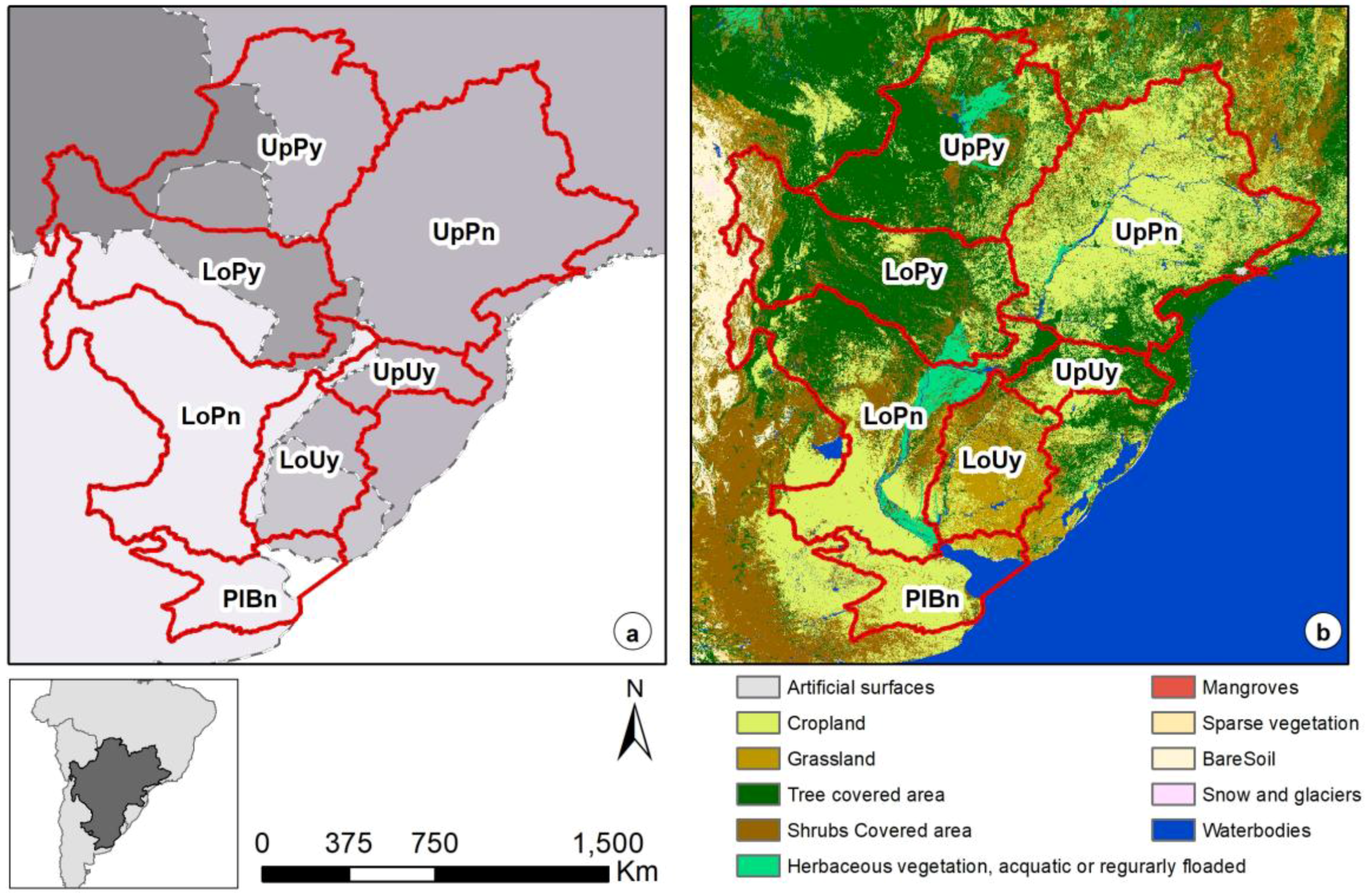
2.1. Data and Regional Extent

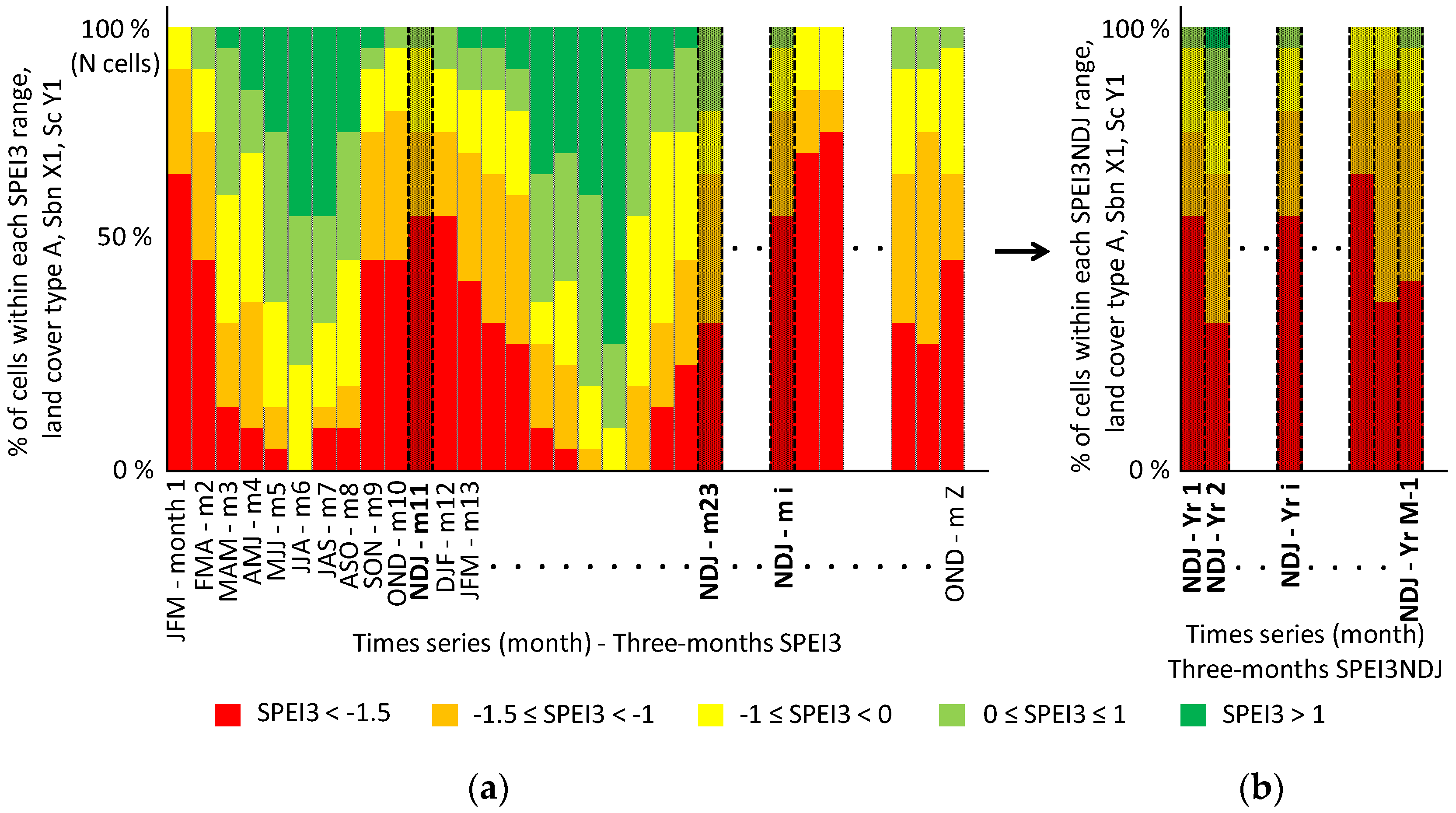
We identified and characterized dry and wet periods within the La Plata Basin (Figure 1) for the current period and future scenarios on a monthly time scale, on a distributed spatial scale, and by using the SPEI [64,65]. The SPEI is based on a monthly climatic water balance D = P – PET, which provides a simple measure of the water surplus or deficit for a specific analysed month. The D values are accumulated at different time scales to obtain different SPEI values (e.g., SPEI1, SPEI3, SPEI6, SPEI12, for 1, 3, 6, and 12 months, respectively, among others). Three-parameter Log-logistic distribution is used to fit the D series, as this distribution shows a gradual decrease in the curve for low values, and coherent probabilities are obtained for very low values of D. The distribution parameters are calculated by applying the probability weighted moments (PWMs) method by means of the unbiased estimator given by Hosking [80], as the standard deviation of the SPEI series does not change among the different SPEI time scales. Then, the probability distribution function of D is calculated according to the Log-logistic distribution (F(x)). The SPEI is obtained as the standardized values of F(x) following the approximation of Abramowitz and Stegun [81]. The average value of the SPEI is 0, and the standard deviation is 1. The SPEI is a standardized variable, and it can therefore be compared with other SPEI values over time and space. For example, an SPEI of 0 indicates a value corresponding to 50% of the cumulative probability of D, according to a Log-logistic distribution. A detailed description of the SPEI can be found in Vicente-Serrano et al. [64].

The three-month SPEI (SPEI3) was chosen in this study as it provides seasonal information. SPEI3 values < 0 were designated as dry periods, whereas SPEI3 values ≥ 0 were designated as wet periods. Moderate to severe droughts were assumed as those dry periods with SPEI3 < −1 (e.g., [63,81,82,83]). According to the WMO and GWP [62], the inclusion of temperature data to calculate PET allows the SPEI to account for the impact of this variable on a drought situation, and it is appropriate when looking at the impact of climate change under various future scenarios. The SPEI3 calculation was based on current and future monthly series of P and PET provided by the INPE. These were estimated using the regional climatic model Eta, which was specifically modelled in the La Plata Basin under the boundary conditions of the HadGEM2-ES model and the moderate CO₂ emissions scenario RCP 4.5 [24,27,51,54,55]. We used data spatially distributed in 0.11 arc degree cells (approximately 10 × 10 km) and temporarily divided into a control period and three future climate scenarios: 1961–2005, 2011–2040, 2041–2070, and 2070–2099, henceforth scenarios Sc0, Sc1, Sc2, and Sc3, respectively. The control period corresponds to a modelled period resulting from previous studies where the Eta model was calibrated and validated with observed climatic series [24,27,51]. It should be noted that all calculations for the analysis of droughts were performed at the cell level and avoiding spatial averaging. We also considered as analysis units the seven sub-basins that comprise the La Plata Basin defined by the Intergovernmental Coordinating Committee of the Countries of the La Plata Basin (CIC) (

Table 1. Characteristics of the sub-basins that comprise the La Plata Basin and percentage of sub-basin area covered by cropland and grassland.

Sub-Basin	Abbreviation	Area	% of Sub-Basin Area
		(km2)	Cropland	Grassland
Upper Paraguay	UpPy	600,086	18	5
Upper Paraná	UpPn	899,628	68	4
Lower Paraguay	LoPy	520,068	12	5
Lower Paraná	LoPn	610,885	38	5
Upper Uruguay	UpUy	116,470	41	4
Lower Uruguay	LoUy	236,980	22	52
La Plata River	PlBn	190,112	75	10
	Total (km2)	3,174,229

and Figure 1a). The sub-basins were named as: Upper Paraguay (UpPy), Upper Paraná (UpPn), Lower Paraguay (LoPy), Lower Paraná (LoPn), Upper Uruguay (UpUy), Lower Uruguay (LoUy), and Río de la Plata (PlBn). Finally, land cover data corresponding to cropland and grassland were extracted from the Global Land Cover-SHARE (FAO) land cover database (Figure 1b, [84]), which is spatially distributed in 0.00833 arc degree cells (approximately 1 × 1 km). We aggregated the land cover data in 0.11 arc degree cells (i.e., the calculation unit) by assigning the land cover value corresponding to the predominant land cover type within each cell. We verified this assumption by comparing, for each defined sub-basin, the area corresponding to each land cover type starting from the 0.11 and 0.00833 arc degree data. We show the mean annual P and PET for each sub-basin and climate scenario in

Table 2. Mean annual precipitation (P) and potential evapotranspiration (PET) of sub-basins that comprise the La Plata Basin for the analysed climate scenarios.

Mean Annual P (mm/Year)
Climate Scenarios	UpPy	UpPn	LoPy	LoPn	UpUy	LoUy	PlBn
1961–2005	1201	1792	1005	1032	2254	1609	1138
2011–2040	1042	1501	963	1112	2478	1795	1309
2041–2070	1167	1780	1105	1220	2781	1878	1279
2071–2099	1226	1848	1170	1270	2914	1961	1294
Mean Annual PET (mm/Year)
Climate Scenarios	UpPy	UpPn	LoPy	LoPn	UpUy	LoUy	PlBn
1961–2005	2579	2169	2243	2113	1825	1820	1780
2011–2040	2916	2532	2407	2074	1915	1802	1687
2041–2070	3008	2513	2466	2158	1962	1874	1809
2071–2099	2983	2527	2407	2126	1952	1863	1797

.

2.2. Data Analysis

Analyses were developed on a monthly time scale and using the 10 × 10 km cells as calculation units for the seven sub-basins comprising the La Plata Basin. As a first approximation to the identification of spatial patterns on P and PET, we analysed the variation with respect to the current period of both variables for the different future time horizons. To this aim, we averaged the monthly values of P and PET in each cell for the entire period comprising each scenario. Afterwards, the variation of each scenario’s PET and P, relative to Sc0, was calculated per cell. We identified the dry and wet periods for the present climate and future scenarios in each cell by using the three-month SPEI (SPEI3). For each climate scenario and each cell, we temporally averaged on the one hand, the 12 SPIE3 values together (corresponding to a cycle of one year) and, on the other hand, the SPEI3 values corresponding to each three-month period separately; that is January, February, and March (SPEI3JFM), February, March, and April (SPEI3FMA), and so on, until the SPIE3 corresponding to December, January, and February (SPEI3DJF).

Afterwards, we analysed the droughts in relation to two key land cover types in the La Plata Basin: cropland and grassland [1]. The land cover types were defined following GLC-SHARE [84]. Cropland (light brown legend in Figure 1b) includes herbaceous crops, woody crops, and multiple or layered crops. The herbaceous crops class is composed of a main layer of cultivated herbaceous plants, including herbaceous crops used for hay, such as soybean, sunflower, wheat, and maize; all the non-perennial crops that do not last for more than two growing seasons; and crops like sugar cane which are regularly harvested while the root system can remain for more than one year in the field. The woody crops class includes a main layer of permanent crops (trees and/or shrub crops) and all types of orchards and plantations (fruit trees, coffee and tea plantation, oil palms, rubber plantation, etc.). Finally, the multiple or layered crops class combines different land covers as two layers of different crops (woody + herbaceous) or the presence of one important layer of natural vegetation (mainly trees) that covers one layer of cultivated crops. Grassland (yellow legend in Figure 1b) includes natural herbaceous plants (grasslands, prairies, steppes, and savannahs) covering more than 10% of the land, irrespective of different human and/or animal activities, such as grazing, selective fire management, etc. Woody plants (trees and/or shrubs) can be present within this cover type when provided they do not exceed 10% of the cover. For each scenario (ScY1 with duration Z months), sub-basin (Sbn X1), land cover type (A), and monthly time step (note that each month represents three consecutive months in the SPEI3), we analysed the probability of occurrence (Figure 2) and the spatial coverage of dry and wet periods of different magnitudes and return periods.

For the probability of occurrence (Figure 2), we specifically analysed the SPEI3 for the months of November, December, and January (SPEI3NDJ) as crops and grasses may be significantly affected by droughts during this three-month period [1]. To simplify, the SPEI3 values were classified according to the magnitude of the dry/wet period: <−1.5 for severe droughts, between −1.5 and −1.0 for moderate droughts, between −1.0 and 0 for light dry periods, between 0 and 1.0 for light wet periods, and >1.0 for moderate to severe wet periods (e.g., [63,81,82]). We calculated the probability that a land cover type within a sub-basin falls into each SPEI3NDJ category during a specific climate scenario period. To do this, we determined the number of cells belonging to each category (coloured areas within each bar; Figure 2a). Second, we selected only the values corresponding to the SPEI3NDJ (dotted bars; Figure 2a) and summed the total number of cells belonging to each category (Figure 2b). Finally, we calculated the percentage of cells within each category (total area of each colour; Figure 2b) from the total number of cells. The total number of cells corresponded to the multiplication of the number of cells from each land cover type within each sub-basin (N cells) by the number of SPEI3NDJ values (i.e., one per year). This procedure allows the synthesis of the dry/wet conditions for each land cover type, sub-basin, and climate scenario, by aggregating cells and avoiding the calculation of spatial averages. To better assess the spatial-temporal droughts for different periods in LPB based on the gridded SPEI3NDJ data, the drought SAF curves were developed and subsequently analysed following Mishra and Singh [67,68] and Mishra and Desai [69]. We first estimated the drought severity based on the values of the SPEI3NDJ. Then, we (1) calculated the drought severity for each year, climate scenario, sub-basin and land use; (2) estimated the drought severity associated with different areal extents (SPEI3NDJ for different total area percentages covered by each land use); (3) selected the probability distribution for each SPEI3NDJ series corresponding to different area extents and land uses; (4) performed a frequency analysis using the selected probability distribution for the drought severity of different areal extents in order to associate drought severity with different return periods; and (5) finally, developed the drought SAF curves for each climate scenario, sub-basin and land use.

2.3. Limitations of the Methodology

Although the data used in this study (mainly P and PET) are based on scientifically-rigorous studies [24,27,51], they result from the application of a single RCM (Eta Model) and a GCM (HadGEM2-ES), thus, the conclusions derived from this study are inextricably affected by the models’ uncertainty. Additionally, we made a series of simplifying assumptions. We did not consider in this study the different water resource management scenarios derived from the operation of the hydraulic infrastructures in each sub-basin. We assumed invariant land cover types in future climate scenarios in our analyses of droughts in relation to cropland and grassland. We based the drought characterization on the use of the SPEI3 and SPEI3NDJ although, in some cases, these periods may not be the most critical for certain crops and specific conditions. For the estimation of the mean SPEI annual cycle, we temporarily averaged the SPEI3 values for each cell to identify dry and/wet periods of different magnitude, however, the averaging may have masked weak or punctual trends. We carefully analysed our results by minimizing comparisons with absolute values as the length of the control climate scenario differs from that of the future scenarios. Finally, although the existence of a drought is an important factor to be considered when evaluating the potential impact of droughts on croplands and grasslands, other factors, which were not analysed in this study, are also key, such as characteristics of soil, surface, and groundwater hydrology, landscape and topography, type of crops, biological and farm/crops management, and climate variables, among others.

3. Results

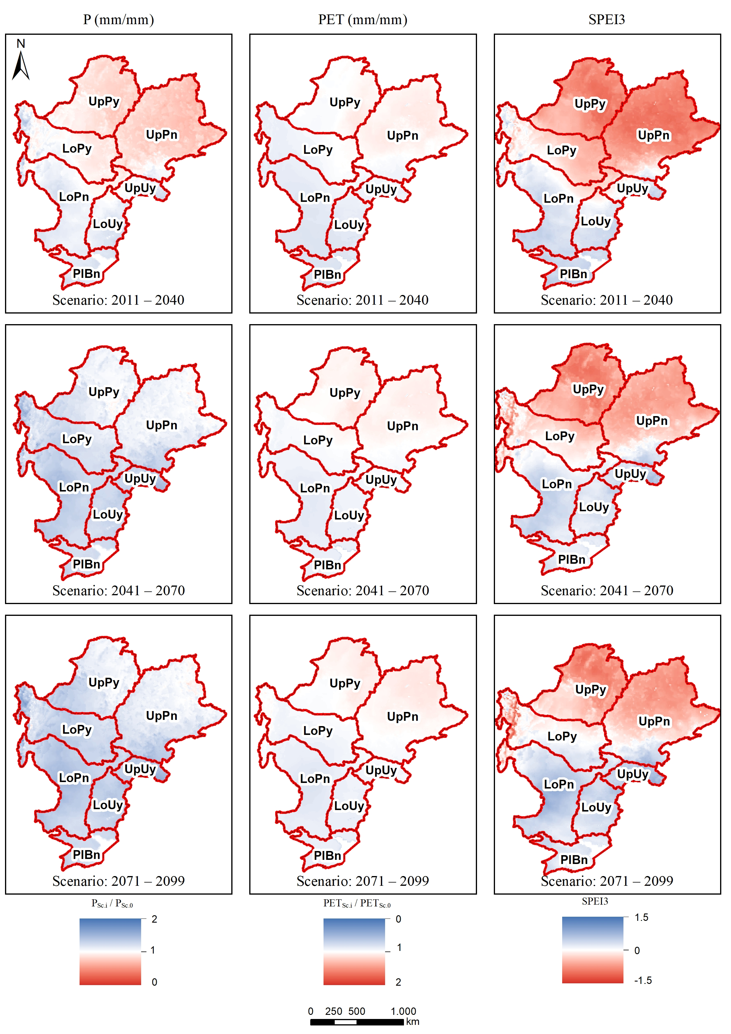
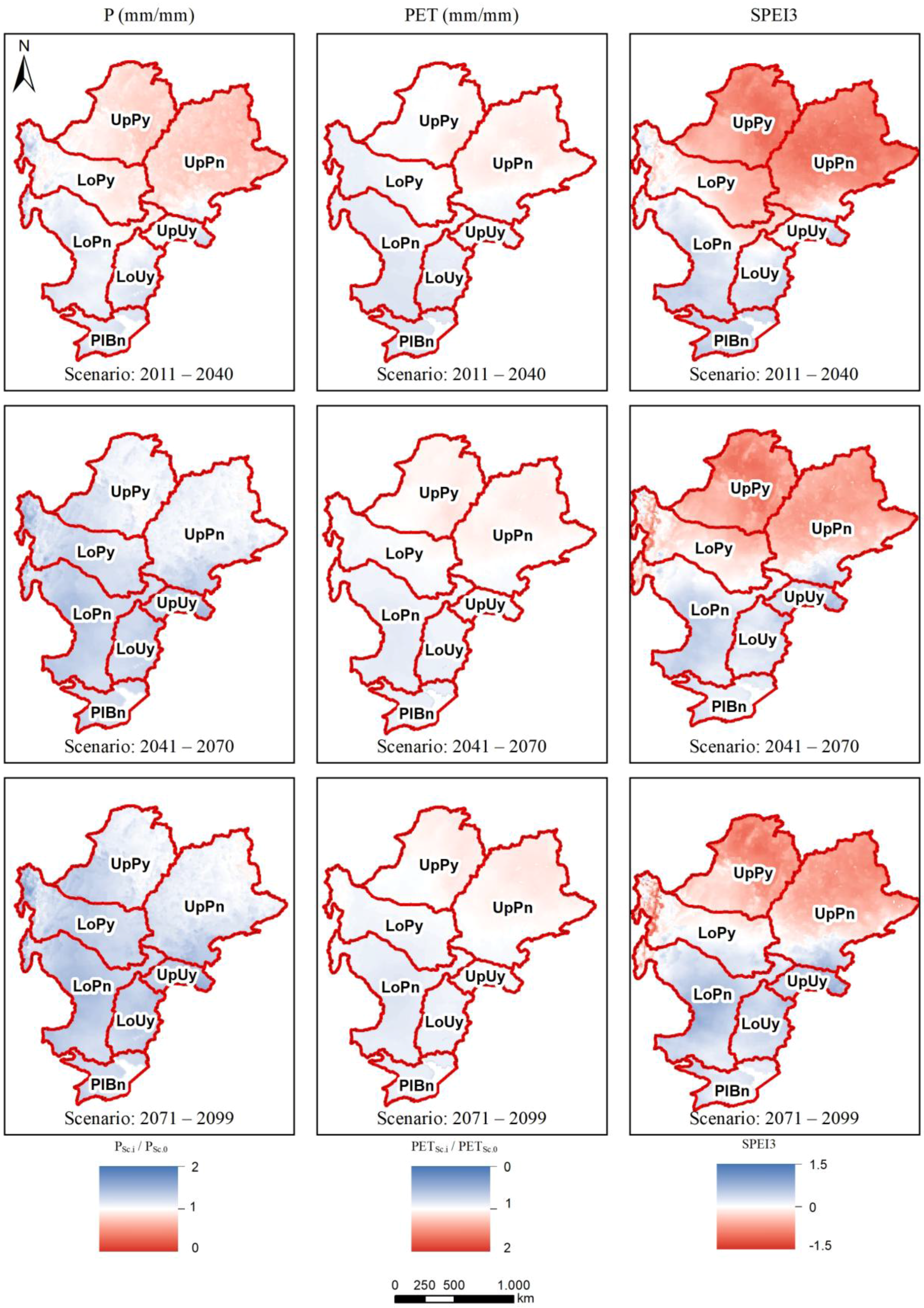
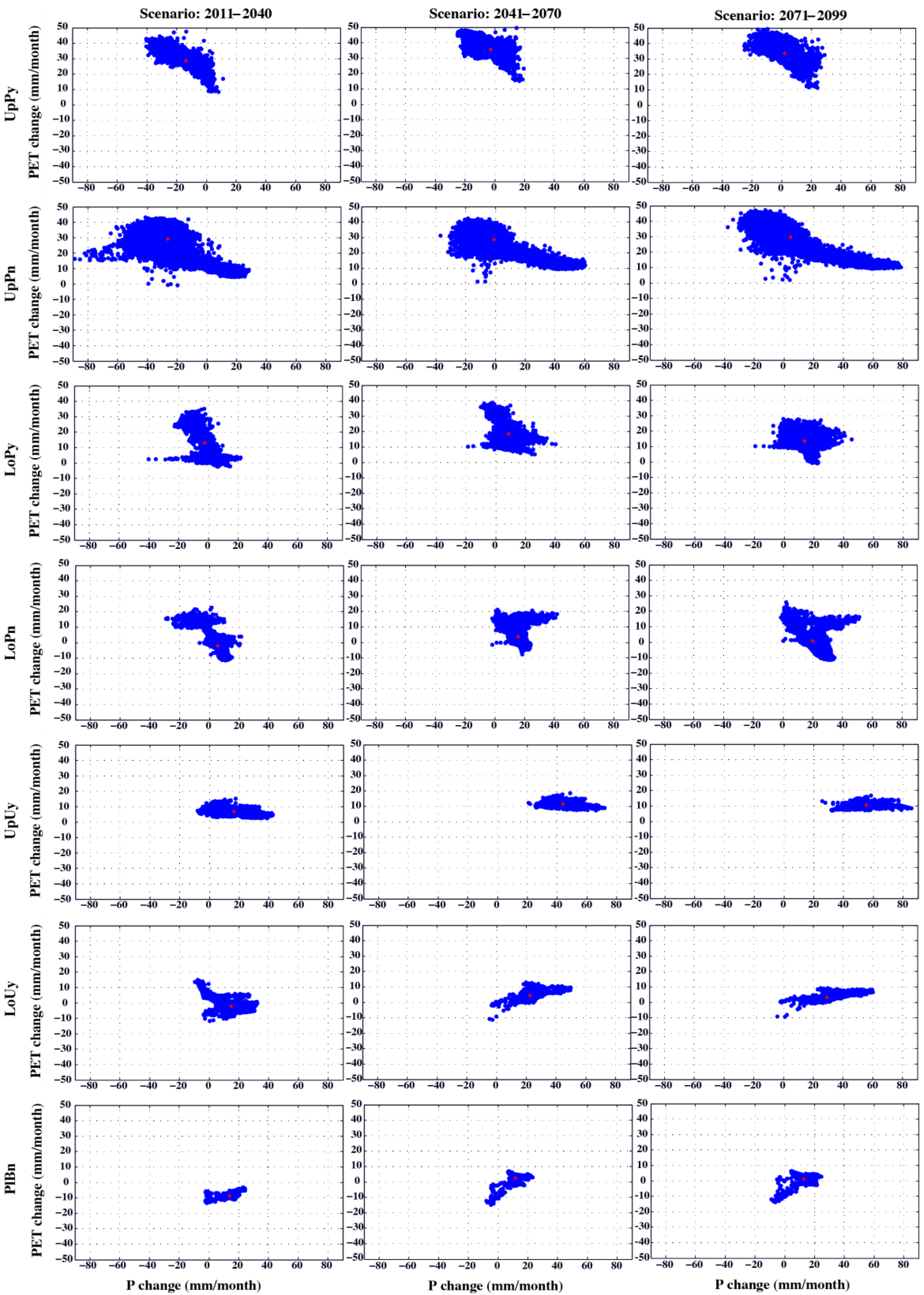
3.1. Precipitation and Evapotranspiration

In the introductory section, the results from the validation of the Eta model for the current period (1961–1990) performed in precedent studies [24,27,51] were shown. In general, the Eta Model was able to capture the spatial and temporal patterns of observed precipitation and temperature. In this study we conducted a complementary analysis. From the monthly CRU database [60] we calculated the mean monthly fluctuation of precipitation for 80 rainfall gauges within the La Plata Basin for the period 1961–2005. We applied the geostatistical method named Kriging and estimated the mean monthly fluctuation of precipitation for each sub-basin. The ranges of the differences between modelled and observed precipitation were, in mm/day: UpPy: 1.55 to −0.86, UpPn: 2.33 to −0.33, LoPy: 0.53 to −1.10, LoPn: 0.70 to −1.35, UpUy: 2.94 to −0.33, LoUy: 1.87 to −0.88, and PlBn: 0.84 to −0.23. The highest difference corresponded to UpUy. Focusing on the NDJ period, the over- and under-estimation was, in mm/day: UpPy: −0.8, UpPn: 0.5, LoPy: −0.5, LoPn: 0.0, UpUy: 1.2, LoUy: 0.9 and PlBn: 0.8. As seen, the results were similar to precedent studies, suggesting that the performance of the models is adequate for the proposed study.

P and PET varied in future scenarios compared to the current period following a marked north–south spatial pattern (Figure 3 and Figure 4). The colours in Figure 3 represent the temporal mean changes of the ratio between P for each cell over the future climate conditions and the P for the current period (same for PET). An increase of P favours less dry (or wetter) climate conditions, whereas an increase of PET favours drier (or less wet) climate conditions. The P temporal mean changes for most cells comprising UpPy, UpPn, and LoPy in Sc1 were negative and became positive in Sc2 and Sc3 (the ratio contained values higher than one, Figure 3). However, certain cells within these sub-basins showed both positive and negative P mean change values for all climate scenarios, which highlights the high spatial variability of this variable (Figure 4). The P temporal mean changes for most of the cells comprising LoPn, UpUy, LoUy, and PlBn were both positive and negative in Sc1 and moved towards positive values in Sc2 and Sc3 (Figure 3). This also showed an important spatial variability within each sub-basin (Figure 4). The PET temporal mean changes for most of the cells comprising UpPy, LoPy, UpPn, and UpUy were positive for all climate scenarios. The PET temporal mean changes for most of the cells comprising LoPn, LoUy and PlBn in Sc1 were negative and moved towards positive values in Sc2 and Sc3 (Figure 3). In general, the spatial variability of the PET mean changes was lower than that of P, and remained similar for all scenarios (Figure 4).

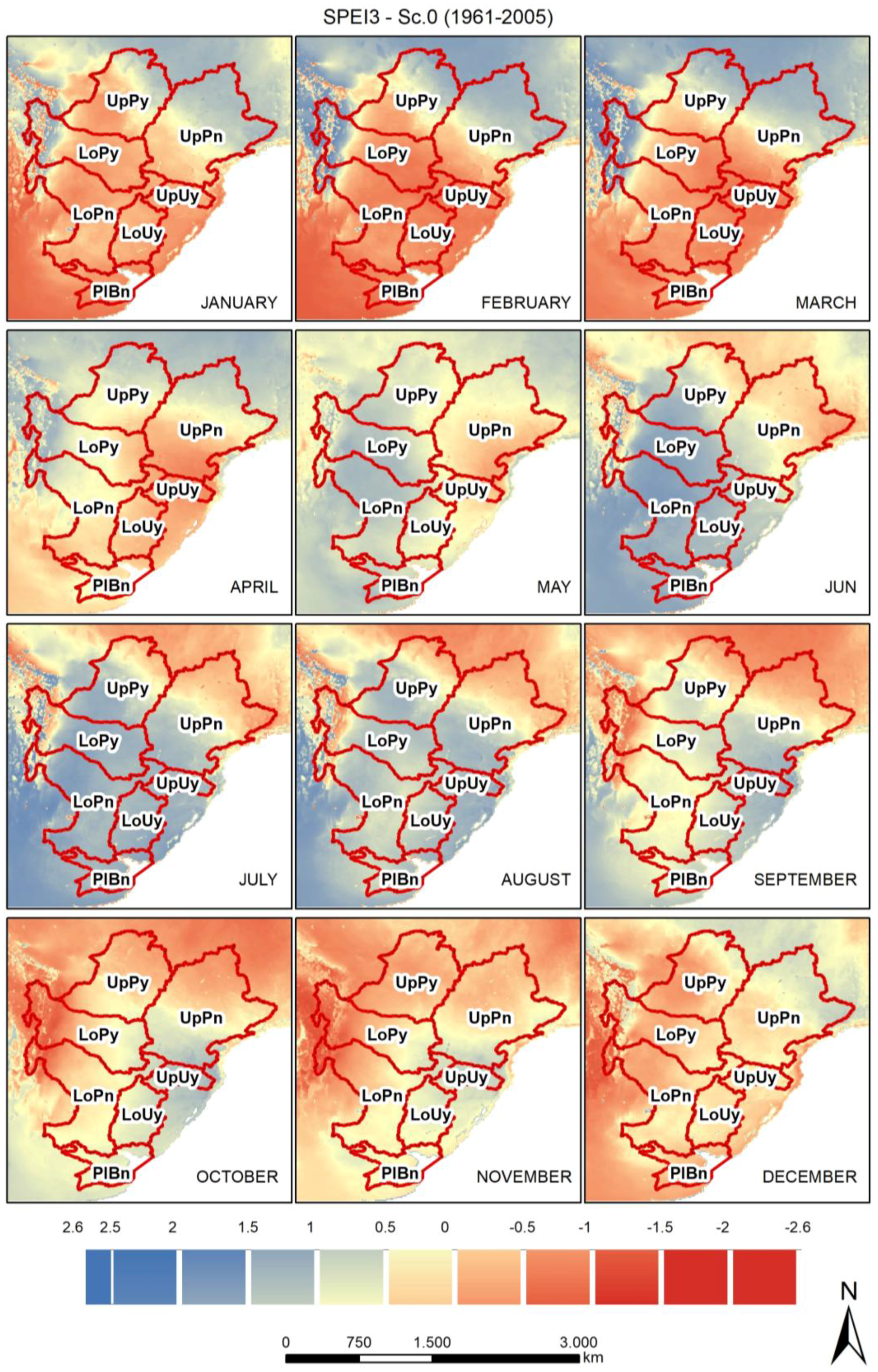
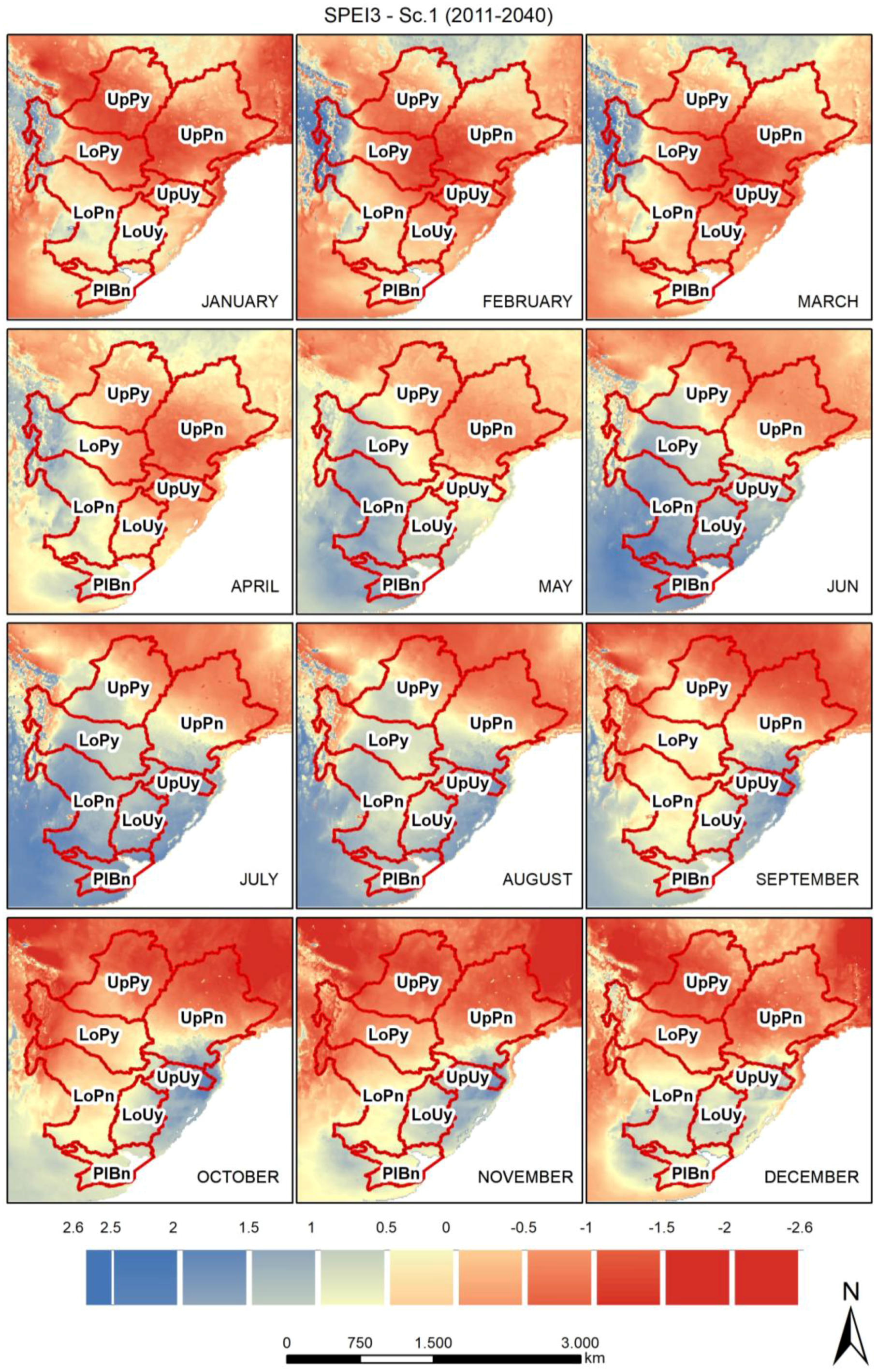
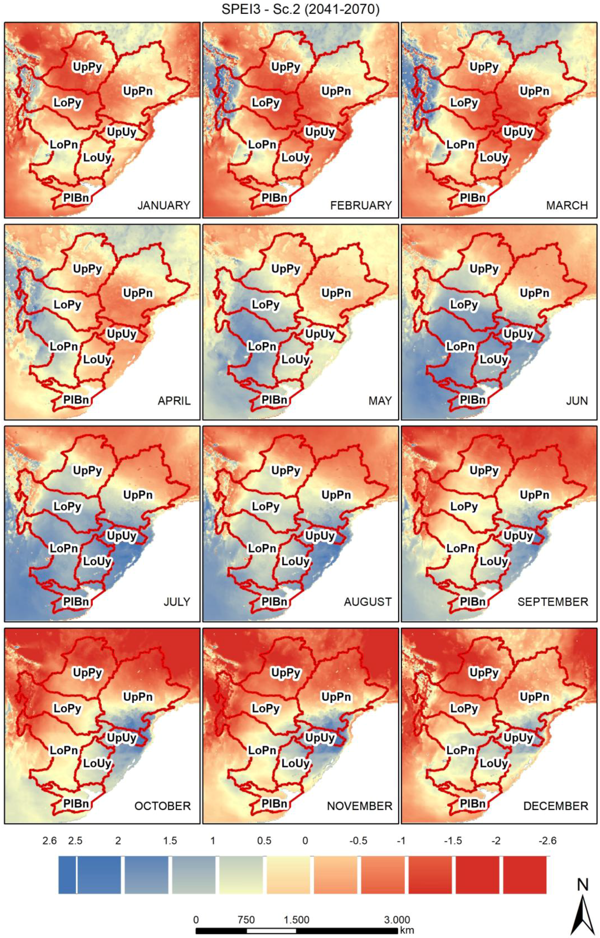
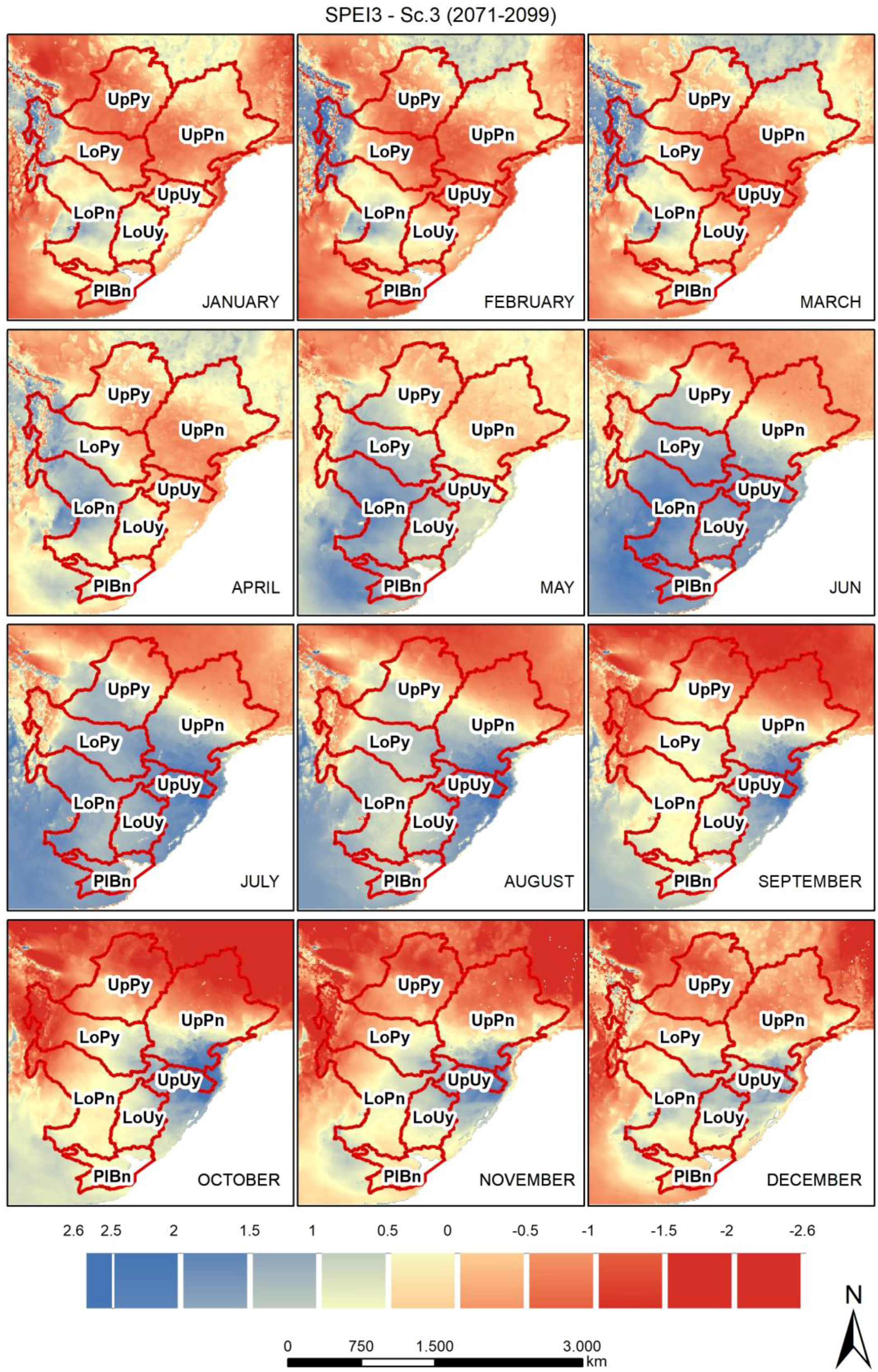
3.2. Three-Month SPEI (SPEI3)

Figure 3 and Figure 6, Figure 7, Figure 8 show SPEI3 variations in future scenarios compared to the current period (Figure 5) following a marked north–south spatial pattern. Climate conditions in all future scenarios were drier (conditioned by PET) in UpPy, UpPn, and LoPy, and wetter (conditioned by P) in the remaining sub-basins. SPEI3 showed an important spatial and temporal variability within each sub-basin throughout the year in all analysed climate scenarios (Figure 5, Figure 6, Figure 7 and Figure 8).

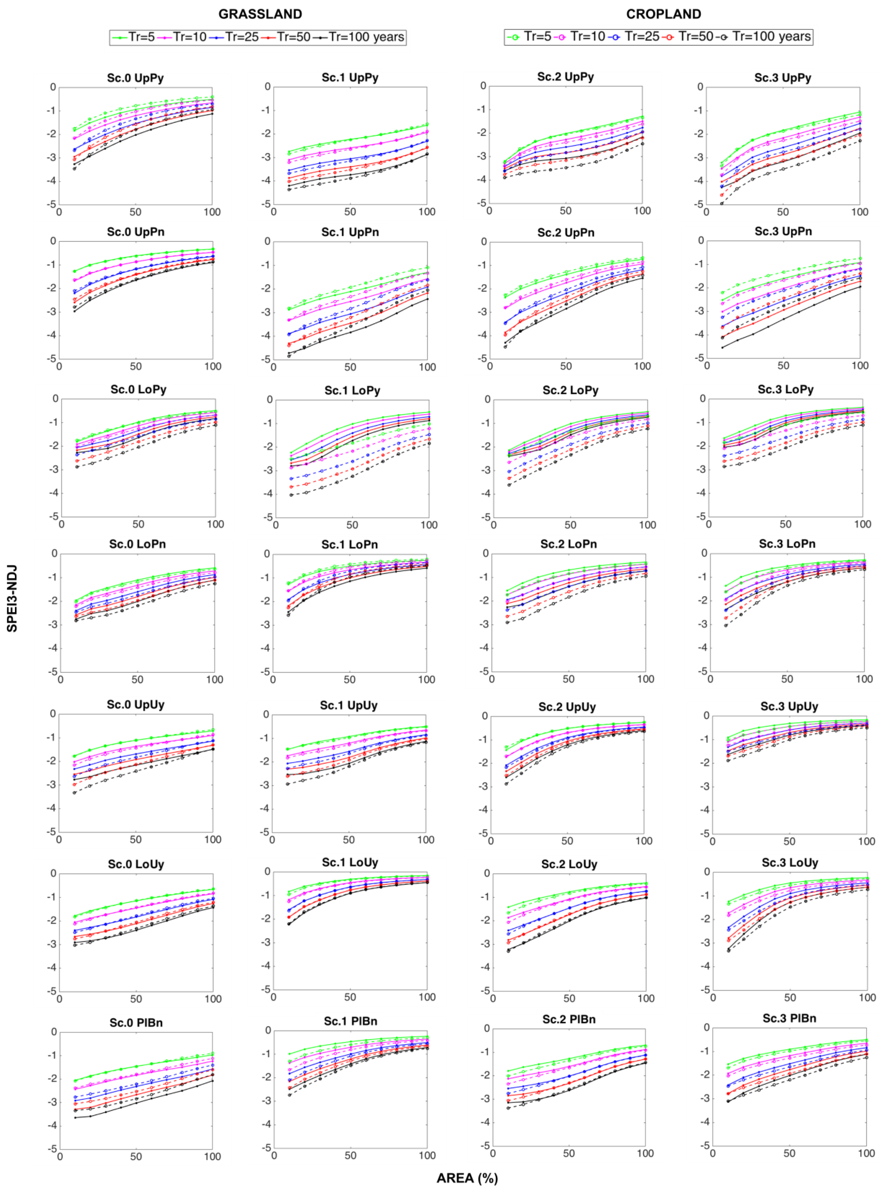
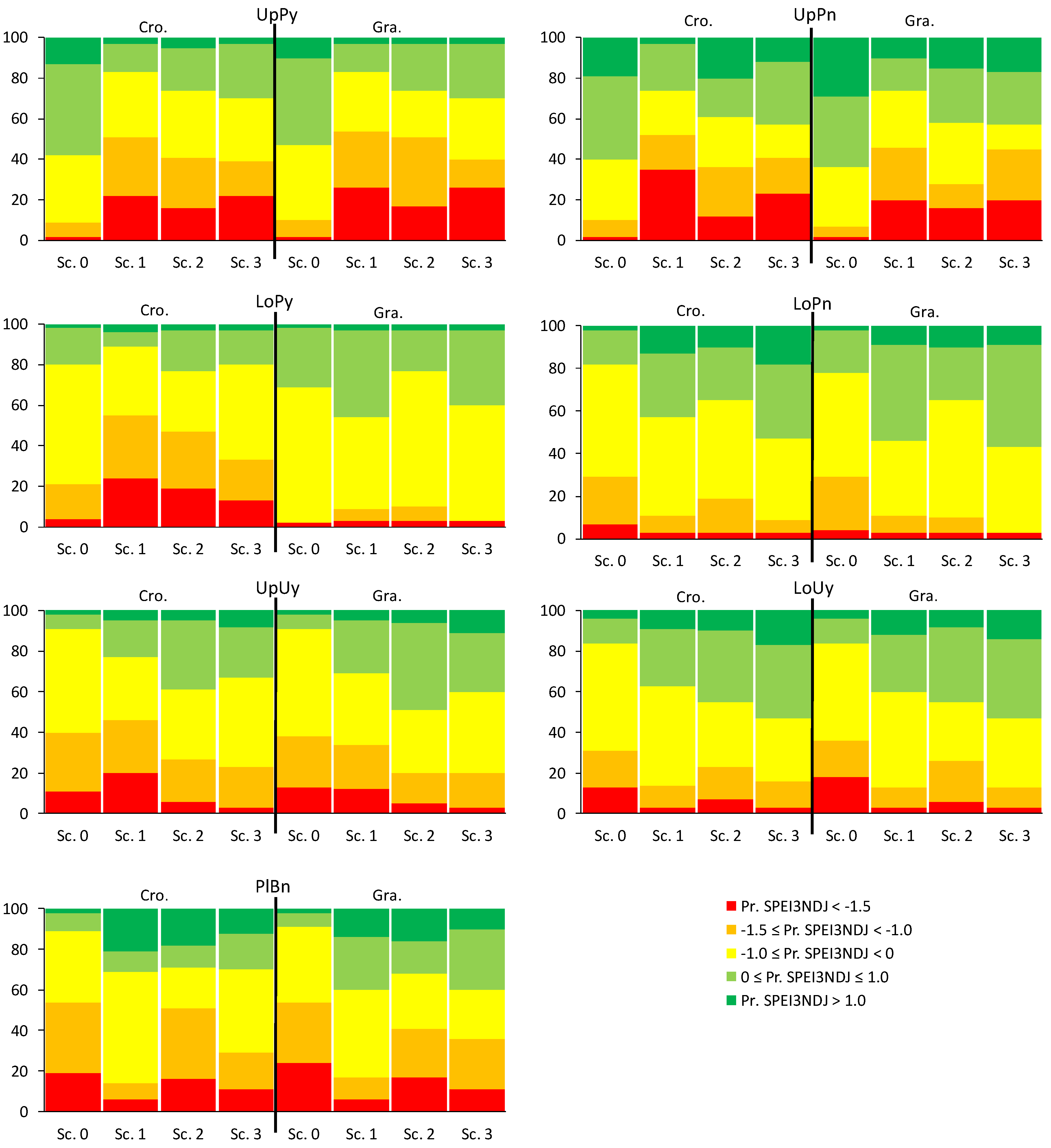
3.3. Seasonal Drought Aspects (Time, Severity, Area and Frequency)

Figure 9 shows the percentages of time (from the total length of each scenario) that the area of each land cover type falls into in each SPEI3NDJ category of dry/wet conditions. In UpPy and UpPn, the percentage of the time of occurrence of both moderate and severe droughts over cropland and grassland areas varied among the sub-basins and scenarios, but it was similar between both land cover types. In UpPy, the likelihood of moderate and severe droughts increased from 9–10% in Sc0 to 52–54% in Sc1, to 41–51% in Sc2, and to 39–40% in Sc3, for cropland and grassland, respectively. In UpPn, moderate and severe droughts increased from 10–7% in Sc0 to 51–47% in Sc1, to 26–28% in Sc2, and 41–45% in Sc3 for cropland and grassland, respectively. In LoPy, relevant differences in relation to the land cover type were found. Meanwhile the likelihood of suffering moderate to severe droughts for the cropland areas increased significantly in the future scenarios (from 21% in Sc0 to 54% in Sc1, to 47% in Sc2, and to 33% in Sc3), and increased slightly (from 2% in Sc0 to 8% in Sc1 and Sc2, and to 3% in Sc3) for grassland areas. In LoPn, moderate and severe droughts occurred in a similar way for both land cover types. Droughts decreased from 29 to 30% in Sc0 to 12–11% for Sc1, from 19 to 11% in Sc2, and from 9 to 3% in Sc3 for cropland and grassland, respectively. In UpUy, moderate and severe droughts slightly increased in Sc1 compared to Sc0 for cropland (40% in Sc0 to 45% in Sc1), and slightly decreased for grassland (38% in Sc0 to 34% in Sc1). Droughts decreased significantly for Sc2, to 27% for cropland and 20% for grassland, and remained the same for Sc3 (23–20%). In LoUy, droughts strongly decreased in Sc1 for cropland and grassland (from 31% in Sc0 to 13% in Sc1, and from 36 to 14%, respectively). In Sc2, the probability of occurrence of moderate and severe droughts was 23% for cropland and 26% for grassland, and in Sc3, 16% for cropland and 13% for grassland. For PlBn, it was 54–55% in Sc0, 14% and 16% in Sc1, 51% and 41% in Sc2, and 29% and 36% for Sc3, for cropland and grassland, respectively (Figure 9).

Figure 10 shows the drought SAF curves for each climate scenario, sub-basin and land use. The future climate scenarios were calculated based on SPEI3NDJ values compared to the series from the current period. In UpPy and UpPn, the drought severity increased for the future scenarios and the areas covered by crops and grasses. Projections show severe droughts for the UpPy and UpPn areas covered by crops and grasses for a return period (Tr) equal or higher than 10 years. In LoPy the behaviour of the drought over cropland and grassland areas differs. While the entire cropland area presents severe droughts for Tr equal to five years, the entire grassland areas present moderate droughts for the entire Tr range analysed (five to 100 years). In LoPn, the areas covered by the analysed land uses are projected to suffer less droughts than in the current period. Nevertheless, more than 20% of the analysed areas are projected to suffer moderate droughts in Sc1 and Sc3 for Tr equal to five years. In Sc2 and Tr equal to five years, more than 30% of the analysed areas with moderate and severe droughts are expected. In UpUy, similar behaviour for Sc0 and Sc1 is expected, that is, more than the 50% of the analysed areas are expected to suffer moderate droughts for Tr equal to five years and severe droughts for Tr equal to 25 years. For Sc2, only 10% and for Sc3 5% of the areas indicate moderate droughts with Tr equal to five years and 50% of the areas with Tr equal to 25 years. In LoUy, the situation improves for the Sc1. In Sc0 more than 60% of the analysed areas are under moderate drought conditions for Tr equal to five years and 50% under severe drought conditions for Tr equal to 10 years. However, for Sc1 drought is not expected for Tr equal to five years and 50% of the cropland and grassland areas showed moderate drought conditions for Tr equal to 50 years. For Sc2 and Tr equal or higher than 25 years, the behaviour is similar to Sc0, however, for Sc2 and lower Tr values, the areas under drought were reduced compared with Sc0. For Sc3, there is an important drought severity variability depending on the considered area. While 30% of the area covered by crops and grasses presents moderate conditions for Tr equal to 10 years, no drought conditions are shown in the whole analysed areas and for Tr equal to 100 years. In PlBn, Sc1 presents better drought conditions compared to Sc0. While for Sc0 the whole area presents moderate droughts for Tr equal to five years, for Sc1 no drought conditions are detected for Tr equal to five years. For Sc2 and Sc3 the behaviour of the drought severity is similar to Sc0.

4. Discussion

Whereas for the far future (2041–2070 and 2071–2099) the projected changes of P and PET were expected to be positive or neutral in most of the La Plata Basin, for the near future (2011–2040) they varied spatially throughout the basin, since P changes negatively in the north and positively in the south, and the opposite is true for PET. PET projections for the scenario 2071–2099 agree with Menendez et al. [37], showing an increase over the northern LPB and a decrease over the southern LPB compared to the current period. Our results for drought partially contrast with Penalba and Rivera [22] who used the SPI as the drought indicator. Unlike the SPEI, the SPI depends exclusively on P, which might somewhat explain why we found drier conditions than the mentioned authors, mainly in the centre and north of the basin where the PET expected changes are more important. In addition, some of the differences could be related to the GCM and RGM used in each study. These results also reveal the importance of the effect of the expected PET changes, accounted for by the SPEI in these regions. In addition, the results reinforce the conclusions stated by the WMO and GWP [62] about the suitability of the use of the SPEI for the study of droughts under climate change conditions. Based on the climate projections, we envisage an increase of droughts in the north of the La Plata Basin and an alternation of wet and short dry periods towards the south in the near future. As more distant future scenarios are analysed, a decrease in the number of droughts from south to north is obtained. However, the high spatial and temporal variability exhibited by droughts when analysed at the cell level reveals that regional analyses, although suited to summarizing general patterns for large regions, run the risk of obviating particular trends.

The fact that the percentage of the area under drought conditions covered by crops was much higher than that covered by grasses in the LoPy sub-basin may be mainly attributed to the specific geographical distribution of the land cover types across this sub-basin and their differing associated climates. In the remaining sub-basins, however, both land cover types were affected in the same manner, despite the high temporal variation of the area under drought conditions. When focusing on the three-month period November, December, and January, differences between land cover types were found in some sub-basins. These results may respond to two reasons. First, both land cover types are located in different regions within each sub-basin and, in some cases (mainly LoPn, UpUy, and PlBn), the extensions dedicated to cropland are higher than those dedicated to grassland. Second, there is great spatial heterogeneity of the appearance of droughts in each sub-basin (mainly LoPy, LoPn, and UpUy). These results highlight the importance of conducting high spatial resolution studies in order to accurately characterize droughts in localized areas and during specific periods.

Mainly in UpPy and UpPn, the projections for all climate scenarios show an increase of moderate and severe droughts over large regions dedicated to crops and grasses. On the other hand, for the near future, in LoUy and PlBn a decrease in drought severity is projected. Changes in agricultural productivity with consequences for food security associated with climate change are expected to exhibit large spatial variability [85]. These changes will vary by crop, region, soil type, and social and economic agent, among others. The projected moderate increase of PET and P in the centre and south of the La Plata Basin might have a positive impact on cropland and grassland, in agreement with the CLARIS LPB project [43] results. Conversely, significant PET rises expected in the north of the basin might negatively impact both land cover types. These projections suggest the need for a potential relocation of certain crops from the northern regions towards cooler regions located in the centre and south. The above suggests likely future effects on grassland and crops, such as their expansion towards marginal regions and an increase in competition among uses in those locations. Actually, in the centre and south of the basin, some authors have already described significant increases of annual crops at the expense of grassland [86], and the expansion of grassland and crops to marginal regions (e.g., [13,78,79]).

Although agricultural systems have their own ability to adapt to climate eventualities [87], the abrupt rate of change expected in these regions, mainly for the near future, could exceed this responsiveness [88]. To deal with this question, adaptation plans should be promoted [13]. Improvement of hydraulic infrastructures [17], cultivation of climate-resilient crop varieties, or management of planting dates to avoid the exposition of the crop to droughts or frosts at the most susceptible stages [2,3,43,89,90,91] are examples of possible adaptation measures. On the other hand, although droughts are widespread in the La Plata Basin, their management is not uniform across the five countries comprising the region. While, in some cases, there are drought monitoring and warning tools, in other cases droughts are undervalued [17]. In this case, analyses like this are important as they provide an overview of the major trends of droughts across large areas, which is particularly useful when managing watersheds that expand across several countries.

5. Conclusions

In this study, we analysed droughts in the La Plata Basin, specifically focusing on regions covered by croplands and grasslands, for different climate scenarios. The following summarizes the key derived conclusions:

• The changes of P and PET (compared to the current period 1961–2005) for the nearest future scenario 2011–2040 showed a marked north–south spatial pattern within the basin. Our results envisage a decrease of rainfall in the north (negative changes of P) but an increase in the south (positive changes of P), and the opposite for PET. An increase of both P and PET (positive changes) are projected for the periods 2041–2070 and 2070–2099 across the whole basin.
• Based on the climate projections, we expect that the north of La Plata Basin will be characterized by an increase of droughts, whereas the south will be dominated by alternating wet and dry periods, during 2011–2040. The wetter climate, however, is expected to spread from south to north in the distant future.
• The high variability of droughts in terms of space, time, and magnitude when analysing at the cell scale highlights the importance of conducting high spatial resolution studies in order to accurately project droughts on localized areas and design tailored measures.
• Only for LoPy were relevant differences in the probability of the occurrence of droughts between cropland and grassland areas found, this being higher in the former.
• Mainly in UpPy and UpPn did the projections for all climate scenarios show an increase of moderate and severe droughts over large regions dedicated to crops and grasses, while for the near future, in LoUy and PlBn the projections show a decrease of drought severity compared to the current period. These projections suggest the need for a potential relocation of certain crops from the northern regions towards cooler regions located in the centre and south, and an increase in competition among uses in these regions.
• When characterizing droughts under a changing climate, it is essential to use indices that involve the relevant climate variables in the study area. In our case, evapotranspiration highly conditions drought occurrence in the north, whereas precipitation is key in the south of the La Plata Basin, thus the SPEI was suitable for this case study.

Regional analyses like ours, although suited to summarizing general patterns for large regions, run the risk of obviating particular behaviours. Further research should conduct high spatial resolution drought studies in localized areas. In addition, different climate projection models should be included. Drought occurrence is one of the various key factors to consider when evaluating the potential impact of droughts on croplands and grasslands. Hence, further research should include the analysis of other factors, such as the characteristics of soils, hydrology, landscape, and topography, the production of different types of crops and grasses, biological and farm/crop management, and other climatic factors. Particularly, each sub-basin’s water use, infrastructure, and available regulation capacity should be included in future studies as they may condition how droughts impact society and how they are managed. It is an important future task to quantitatively evaluate the degree of satisfaction with the current and future water demands and to analyse the regulatory requirements to meet different levels of demand. In order to move towards a successful integrated drought management plan, it would be essential to have a primary integrated regional vision of the current situation in the sub-basins and the need for new facilities based on different future climate scenarios.

References

1. Aquastat. Available online: http://www.fao.org/nr/aquastat (accessed on 1 September 2017).
2. Viglizzo, E.F.; Frank, F.C. Land-use options for Del Plata Basin in South America: Tradeoffs analysis based on ecosystem service provision. Ecol. Econ. 2006, 57, 140–151. [Google Scholar] [CrossRef]
3. Barrucand, M.G.; Vargas, W.M.; Rusticucci, M.M. Dry conditions over Argentina and the related monthly circulation patterns. Meteorol. Atmos. Phys. 2007, 98, 99–114. [Google Scholar] [CrossRef]
4. Llano, M.; Penalba, O. A climatic analysis of dry sequences in Argentina. Int. J. Climatol. 2010, 31, 504–513. [Google Scholar] [CrossRef]
5. Chen, J.; Wilson, C.; Tapley, B.; Longuevergne, L.; Scanlon, B. Recent La Plata basin drought conditions observed by satellite gravimetry. J. Geophys. Res. 2010, 115, D22108. [Google Scholar] [CrossRef]
6. Abelen, S.; Seitz, F.; Abarca-del-Rio, R.; Güntner, A. Droughts and Floods in the La Plata Basin in Soil Moisture Data and GRACE. Remote Sens. 2015, 7, 7324–7349. [Google Scholar] [CrossRef]
7. Penalba, O.; Rivera, J. Comparación de seis índices para el monitoreo de sequías meteorológicas en el Sur de Sudamérica. Meteorologica 2015, 40, 33–57. [Google Scholar]
8. World Water Assessment Programme (WWAP). La Plata Basin Case Study: Final Report; UNESCO: Perugia, Italy, 2007; pp. 1–537. Available online: http://unesdoc.unesco.org/images/0015/001512/151252e.pdf (accessed on 2 November 2017).
9. Penalba, O.; Vargas, W. Review: Variability of low monthly rainfall in La Plata Basin. Meteorol. Appl. 2008, 15, 313–323. [Google Scholar] [CrossRef]
10. Minetti, J.L.; Vargas, W.M.; Poblete, A.G.; Acuña, L.R.; Casagrande, G. Non-linear trends and low frequency oscillations in annual precipitation over Argentina and Chile, 1931–1999. Atmosfera 2004, 16, 119–135. [Google Scholar]
11. Marengo, J.; Bernasconi, M. Regional differences in aridity/drought conditions over Northeast Brazil: Present state and future projections. Clim. Chang. 2015, 129, 103–115. [Google Scholar] [CrossRef]
12. Vargas, W.M.; Naumann, G.; Minetti, J.L. Dry spells in the River Plata Basin: An approximation of the diagnosis of droughts using daily data. Theor. Appl. Climatol. 2011, 104, 159–173. [Google Scholar] [CrossRef]
13. Magrin, G.O.; Marengo, J.A.; Boulanger, J.P.; Buckeridge, M.S.; Castellanos, E.; Poveda, G.; Scarano, F.R.; Vicuña, S. Central and South America. In Climate Change 2014: Impacts, Adaptation, and Vulnerability. Part B: Regional Aspects; Contribution of Working Group II to the Fifth Assessment Report of the Intergovernmental Panel on Climate Change; Barros, V.R., Field, C.B., Eds.; Cambridge University Press: Cambridge, UK; New York, NY, USA, 2014; pp. 1499–1566. [Google Scholar]
14. Doyle, M.E.; Saurral, R.I.; Barros, V.R. Trends in the distributions of aggregated monthly precipitation over the La Plata Basin. Int. J. Climatol. 2012, 32, 2149–2162. [Google Scholar] [CrossRef]
15. Penalba, O.; Robledo, F. Spatial and temporal variability of the frequency of extreme daily rainfall regime in the La Plata Basin during the 20th century. Clim. Chang. 2010, 98, 531–550. [Google Scholar] [CrossRef]
16. Dufek, A.S.; Ambrizzi, T.; Da Rocha, R.P. Are reanalysis data useful for calculating climate indices over South America? Ann. N.Y. Acad. Sci. 2008, 1146, 87–104. [Google Scholar] [CrossRef] [PubMed]
17. Tucci, C. Visão dos Recursos Hídricos da Bacia do Rio da Prata; Visão Regional, Volume 1; GEF-CIC-PNUMA-OEA: Porto Alegre, Brazil, 2004; pp. 1–227. Available online: http://rhama.com.br/blog/wp-content/uploads/2017/04/REGAv3n2.pdf (accessed on 2 November 2017).
18. Valente, M. Agriculture-Argentina: Worst Drought in 100 Years. IPS Online. 21 January 2009, p. 449. Available online: http://www.ipsnews.net/2009/01/agriculture-argentina-worst-drought-in-100-years/ (accessed on 2 November 2017).
19. EM-DAT. International Disaster Database. OFDA/CRED, Université Catholique de Louvain: Brussels, Belgium. Available online: www.emdat.be (accessed on 1 March 2017).
20. Donat, M.G.; Alexander, L.V.; Yang, H.; Durre, I.; Vose, R.; Dunn, R.J.H.; Willett, K.M.; Aguilar, E.; Brunet, M.; Caesar, J.; et al. Updated analyses of temperature and precipitation extreme indices since the beginning of the twentieth century: The HadEX2 dataset. J. Gephys. Res. 2013, 20, 1–16. [Google Scholar] [CrossRef]
21. Caffera, R.M.; Berbery, E.H. La Plata Basin climatology. In Climate Change in the La Plata Basin; Barros, V., Clarke, R., Eds.; Research Centre for Sea and Atmosphere, Cima-Conicet/FCEN-UBA: Buenos Aires, Argentina, 2006; pp. 16–34. [Google Scholar]
22. Penalba, O.; Rivera, J. Regional aspects of future precipitation and meteorological drought characteristics over Southern South America projected by a CMIP5 multi-model ensemble. Am. J. Clim. Chang. 2013, 2, 173–182. [Google Scholar] [CrossRef]
23. Solman, S. Regional climate modelling over South America: A Review. Adv. Meteorol. 2013, 2013, 504357. [Google Scholar] [CrossRef]
24. Chou, S.C.; Lyra, A.; Mourão, C.; Dereczynski, C.; Pilotto, I.; Gomes, J.; Bustamante, J.; Tavares, P.; Silva, A.; Rodrigues, D.; et al. Assessment of Climate Change over South America under RCP 4.5 and 8.5 Downscaling Scenarios. Am. J. Clim. Chang. 2014, 3, 512–527. [Google Scholar] [CrossRef]
25. Llopart, M.; Coppola, E.; Giorgi, F.; da Rocha, R.; Cuadra, S. Climate change impact on precipitation for the Amazon and La Plata basins. Clim. Chang. 2014, 125, 111–125. [Google Scholar] [CrossRef]
26. Marengo, J.; Chou, S.; Alves, L.; National Institute for Space Research. Personal communication, 2014.
27. Mourao, C. Producto 2: Relatório Contendo a Análise das Simulações do Modelo Eta-10 km Para a Região da Bacia do Prata, Utilizando as Condições do HadGEM2-ES RCP 4.5, Para o Período de 1961–2100; Organización de Estados Americanos: Porto Alegre, Brasil, 2014; p. 28. [Google Scholar]
28. Reboita, M.; Da Rocha, R.; Dias, C.; Ynoue, R. Climate Projections for South America: RegCM3 driven by HadCM3 and ECHAM5. Adv. Meteorol. 2014, 2014, 376738. [Google Scholar] [CrossRef]
29. Barros, V.R.; Garavaglia, C.R.; Doyle, M.E. Twenty-first century projections of extreme precipitations in the Plata Basin. Int. J. River Basin Manag. 2013, 11, 373–387. [Google Scholar] [CrossRef]
30. Menéndez, C.G.; Carril, A.F. Potential changes in extremes and links with the Southern Annular Mode as simulated by a multi-model ensemble. Clim. Chang. 2010, 98, 359–377. [Google Scholar] [CrossRef]
31. Jones, C.; Carvalho, L.M.V. Climate change in the South American monsoon system: Present climate and CMIP5 projections. J. Clim. 2013, 26, 6660–6678. [Google Scholar] [CrossRef]
32. Marengo, J.A.; Chou, S.C.; Kay, G.; Alves, L.M.; Pesquero, J.F.; Soares, W.R.; Santos, D.C.; Lyra, A.; Sueiro, G.; Betts, R.; et al. Development of regional future climate change scenarios in South America using the Eta CPTEC/HadCM3 climate change projections: Climatology and regional analyses for the Amazon, São Francisco and the Parana River Basins. Clim. Dyn. 2011, 38, 1829–1848. [Google Scholar] [CrossRef]
33. Cavalcanti, I.F.A. Large scale and synoptic features associated with extreme precipitation over South America: A review and case studies for the first decade of the 21st century. Atmos. Res. 2012, 118, 27–40. [Google Scholar] [CrossRef]
34. Cavalcanti, I.F.A.; Carril, A.F.; Penalba, O.C.; Grimm, A.M.; Menéndez, C.G.; Sanchez, E.; Cherchi, A.; Sörensson, A.; Robledo, F.; Rivera, J.; et al. Flach Precipitation extremes over La Plata Basin—Review and new results from observations and climate simulations. J. Hydrol. 2015, 523, 211–230. [Google Scholar] [CrossRef]
35. Chou, S.C.; Tanajura, C.A.S.; Xue, Y.; Nobre, C.A. Validation of the coupled Eta/SSiB model over South America. J. Geophys. Res. 2002, 107, LBA56-1–LBA56-20. [Google Scholar] [CrossRef]
36. Carril, A.F.; Menéndez, C.G.; Remedio, A.R.C.; Robledo, F.; Sörenson, A.; Tencer, B.; Boulanger, J.P.; de Castro, M.; Jacob, D.; Le Treut, H.; et al. Performance of a multi-RCM ensemble for South Eastern South America. Clim. Dyn. 2012, 39, 2747–2768. [Google Scholar] [CrossRef]
37. Menéndez, C.G.; Zaninelli, P.; Carril, A.; Sánchez, E. Hydrological cycle, temperature, and land surface atmosphere interaction in the La Plata Basin during summer: Response to climate change. Clim. Res. 2016, 68, 231–241. [Google Scholar] [CrossRef]
38. Solman, S.; Sánchez, E.; Samuelsson, R.P.; Da Rocha, C.; Marengo, J.; Pessacg, N.L.; Remedio, A.R.C.; Chou, S.C.; Berbery, H.; Le Treut, H.; et al. Evaluation of an ensemble of regional climate model simulations over South America driven by the ERA-Interim reanalysis: Model performance and uncertainties. Clim. Dyn. 2013, 41, 1139–1157. [Google Scholar]
39. Menéndez, C.G.; De Castro, M.; Boulanger, J.P.; D’Onofrio, A.; Sánchez, E.; Sörenson, A.A.; Blázquez, J.; Elizalde, J.; Jacob, D.; Li, Z.X.; et al. Downscaling extreme month-long anomalies in southern South America. Clim. Chang. 2010, 98, 379–403. [Google Scholar] [CrossRef]
40. Solman, S.A.; Pessacg, N.-L. Evaluating uncertainties in regional climate simulations over South America at the seasonal scale. Clim. Dyn. 2012, 39, 59–76. [Google Scholar] [CrossRef]
41. Parker, W.S. Ensemble modeling, uncertainty and robust predictions. WIREs Clim. Chang. 2013, 4, 213–223. [Google Scholar] [CrossRef]
42. Sánchez, E.; Solman, S.; Remedio, A.R.C.; Berbery, H.; Samuelsson, R.P.; Da Rocha, C.; Mourão, L.; Marengo, J.; De Castro, M.; Jacob, D.; et al. Regional climate modelling in CLARIS-LPB: A concerted approach towards twenty first century projections of regional temperature and precipitation over South America. Clim. Dyn. 2015, 45, 2193–2212. [Google Scholar] [CrossRef]
43. Claris LPB. A Europe-South America Network for Climate Change Assessment and ImStudies in La Plata Basin. FP7-ENVIRONMENT—Specific Programme “Cooperation”: Environment (Including Climate Change). Project ID: 212492. Available online: http://cordis.europa.eu/project/rcn/89402_en.html (accessed on 2 November 2017).
44. Simmons, A.; Uppala, S.; Dee, D.; Kobayashi, S. ERA-interim: New ECMWF reanalysis products from 1989 onwards. ECMWF Newsl. 2007, 110, 25–35. [Google Scholar]
45. Chen, M.; Shi, W.; Xie, P.; Silva, V.B.S.; Kousky, V.E.; Higgins, R.W.; Janowiak, J.E. Assessing objective techniques for gauge-based analyses of global daily precipitation. J. Geophys. Res. 2008, 113, D04110. [Google Scholar] [CrossRef]
46. Mesinger, F.; Veljovic, K.; Chou, S.C.; Gomes, J.; Lyra, A. The Eta Model: Design, Use, and Added Value. In Topics in Climate Modeling; Chapter 6; Intech: Rijeka, Croatia; Available online: http://www.intechopen.com/books/topics-in-climate-modeling (accessed on 2 November 2017).
47. Chou, S.C.; Fonseca, J.F.; Gomes, J.L. Evaluation of Eta Model seasonal precipitation forecasts over South America. Nonlinear Proc. Geophys. 2005, 12, 537–555. [Google Scholar] [CrossRef]
48. Mesinger, F.; Chou, S.; Gomes, J.; Jovic, D.; Bastos, P.; Bustamante, J.F.; Lazic, L.; Lyra, A.A.; Morelli, S.; Ristic, I.; et al. An upgraded version of the Eta model. Meteorol. Atmos. Phys. 2012, 116, 63–79. [Google Scholar] [CrossRef]
49. Mesinger, F.; Janjic, Z.I. Noise Due to Time-Dependent Boundary Conditions in Limited Area Models. The GARP Programme on Numerical Experimentation; Rep. No. 4; WMO: Geneva, Switzerland, 1974; pp. 31–32. [Google Scholar]
50. Black, T.L. The New NMC mesoscale Eta model: Description and forecast samples. Weather Forecast. 1994, 9, 256–278. [Google Scholar] [CrossRef]
51. Chou, S.C.; Lyra, A.A.; Mourão, C.; Dereczynski, C.; Pilotto, I.; Gomes, J.; Bustamante, J.; Tavares, P.; Silva, A.; Rodrigues, D.; et al. Evaluation of the Eta Simulations Nested in Three Global Climate Models. Am. J. Clim. Chang. 2014, 3, 438–454. [Google Scholar] [CrossRef]
52. Chou, S.; Marengo, J.; Lyra, A.A.; Sueiro, G.; Pesquero, J.F.; Alves, L.M.; Kay, G.; Betts, R.; Chagas, D.J.; Gomes, J.L.; et al. Downscaling of South America present climate driven by 4-member HadCM3 runs. Clim. Dyn. 2012, 38, 635–653. [Google Scholar] [CrossRef]
53. Pesquero, J.F.; Chou, S.; Nobre, C.A.; Marengo, J.A. Climate downscaling over South America for 1961–1970 using the Eta Model. Theor. Appl. Climatol. 2010, 99, 75–93. [Google Scholar] [CrossRef]
54. Bustamante, J.F.; Gomes, J.L.; Chou, S.C. 5-year Eta Model Seasonal Forecast Climatology over South America. In Proceedings of the International Conference on Southern Hemisphere Meteorology and Oceanography, Foz do Iguaçu, Brazil, 24–28 April 2006; pp. 503–506. [Google Scholar]
55. Alves, L.F.; Marengo, J.A.; Chou, S.C. Avaliação das Previsões de Chuvas Sazonais do Modelo Eta Climático Sobre o Brasil. In Proceedings of the Congresso Brasiliero de Meteorologia, Fortaleza, Brazil, 29 August–13 October 2004. [Google Scholar]
56. Chou, S.C.; Nunes, A.M.B.; Cavalcanti, I.F.A. Extended range forecasts over South America using the regional Eta model. J. Geophys. Res. 2000, 105, 10147–10160. [Google Scholar] [CrossRef]
57. Bellouin, N.; Rae, J.; Jones, A.; Johnson, C.; Haywood, J.; Boucher, O. Aerosol forcing in the Climate Model Intercomparison Project (CMIP5) simulations by HadGEM2-ES and the role of ammonium nitrate. J. Geophys. Res. 2011, 116, 1–25. [Google Scholar] [CrossRef]
58. Collins, W.J.; Bellouin, N.; Doutriaux-Boucher, M.; Gedney, N.; Halloran, P.; Hinton, T.; Hughes, J.; Jones, C.D.; Joshi, M.; Liddicoat, S.; et al. Development and evaluation of an Earth-System model HadGEM2. Geosci. Model Dev. 2011, 4, 1051–1075. [Google Scholar] [CrossRef]
59. Martin, G.M.; Bellouin, N.; Collins, W.J.; Culverwell, I.D.; Halloran, P.R.; Hardiman, S.C.; Hinton, T.J.; Jones, C.D.; McDonald, R.E.; McLaren, A.J.; et al. The HadGEM2 family of Met Office Unified Model climate configurations. Geosci. Model Dev. 2011, 4, 723–757. [Google Scholar]
60. University of East Anglia Climatic Research Unit (CRU). CRU TS Version 3.22. Climatic Research Unit (CRU) Time-Series Datasets of Variations in Climate with Variations in Other Phenomena; Climatic Research Unit, NCAS British Atmospheric Data Centre: Norwich, UK, 2014. [Google Scholar]
61. Thomson, A.M.; Calvin, K.V.; Smith, S.J.; Kyle, G.P.; Volke, A.; Patel, P.; Delgado-Arias, S.; Bond-Lamberty, B.; Wise, M.A.; Clarke, L.E.; et al. RCP4.5: A pathway for stabilization of radiative forcing by 2100. Clim. Chang. 2011, 109, 77–94. [Google Scholar] [CrossRef]
62. World Meteorological Organization (WMO) and Global Water Partnership (GWP). Handbook of Drought Indicators and Indices; Integrated Drought Management Programme (IDMP), Integrated Drought Management Tools and Guidelines Series 2; Svoboda, M., Fuchs, B.A., Eds.; WMO: Geneva, Switzerland, 2016; pp. 1–52. [Google Scholar]
63. World Meteorological Organization (WMO). Standardized Precipitation Index. User Guide; World Meteorological Organization: Geneva, Switzerland, 2012; pp. 1–24. [Google Scholar]
64. Vicente-Serrano, S.M.; Beguería, S.; López-Moreno, J.I. A Multi-scalar drought index sensitive to global warming: The Standardized Precipitation Evapotranspiration Index—SPEI. J. Clim. 2010, 23, 1696–1718. [Google Scholar] [CrossRef]
65. Beguería, S.; Vicente-Serrano, S.M.; Angulo, M. A multi-scalar global drought data set: The SPEIbase: A new gridded product for the analysis of drought variability and impacts. Am. Meteorol. Soc. 2010, 91, 1351–1354. [Google Scholar] [CrossRef]
66. Hao, Z.; Singh, V. Drought characterization from a multivariate perspective: A review. J. Hydrol. 2015, 527, 668–678. [Google Scholar] [CrossRef]
67. Mishra, A.; Singh, V. Drought modeling—A review. J. Hydrol. 2011, 403, 157–175. [Google Scholar] [CrossRef]
68. Mishra, A.; Singh, V. Analysis of drought severity-area-frequency curves using a general circulation model and scenario uncertainty. J. Geophys. Res. 2009, 114, D06120. [Google Scholar] [CrossRef]
69. Mishra, A.; Desai, V. Spatial and temporal drought analysis in the Kansabati River Basin, India. Int. J. River Basin Manag. 2005, 3, 31–41. [Google Scholar] [CrossRef]
70. Loukas, A.; Vasiliades, L. Probabilistic analysis of drought spatiotemporal characteristics in Thessaly region, Greece. Nat. Hazards Earth Syst. 2004, 4, 719–731. [Google Scholar] [CrossRef]
71. Bonaccorso, B.; Peres, D.J.; Castano, A.; Cancelliere, A. SPI-Based Probabilistic Analysis of Drought Areal Extent in Sicily. Water Resour. Manag. 2015, 29, 459–470. [Google Scholar] [CrossRef]
72. Kim, T.; Valdés, J. Frequency and Spatial Characteristics of Droughts in the Conchos River Basin, Mexico. Water Int. 2002, 27, 420–430. [Google Scholar] [CrossRef]
73. Gregg, J.S.; Smith, S.J. Global and regional potential for bioenergy from agricultural and forestry residue biomass. Mitig. Adapt. Strat. Glob. Chang. 2010, 15, 241–262. [Google Scholar] [CrossRef]
74. Barros, V. Adaptation to climate trends: Lessons from the Argentine experience. In Climate Change and Adaptation; Leary, N., Adejuwon, J., Eds.; Earthscan: London, UK; New York, NY, USA, 2008; pp. 296–314. [Google Scholar]
75. Podestá, G.; Bert, F.; Rajagopalan, B.; Apipattanavis, S.; Laciana, C.; Weber, E.; Easterling, W.; Katz, R.; Letson, D.; Menéndezs, A. Decadal climate variability in the Argentine Pampas: Regional impacts of plausible climate scenarios on agricultural systems. Clim. Res. 2009, 40, 199–210. [Google Scholar] [CrossRef]
76. Hoyos, L.E.; Cingolani, A.M.; Zak, M.-R.; Vaieretti, M.V.; Gorla, D.E.; Cabido, M.R. Deforestation and precipitation patterns in the arid Chaco forests of central Argentina. Appl. Veg. Sci. 2012, 16, 260–271. [Google Scholar] [CrossRef]
77. Schlindwein, S.; Sieber, S. CLARIS LPB WP8: Land Use Change, Agriculture and Socio-Economic Implications. CLIVAR Exch. 2011, 57, 28–31. [Google Scholar]
78. Wassenaar, T.; Gerber, P.; Verburg, P.H.; Rosales, M.; Ibrahim, M.; Steinfeld, H. Projecting land use changes in the Neotropics: The geography of pasture expansion into forest. Glob. Environ. Chang. 2007, 17, 86–104. [Google Scholar] [CrossRef]
79. Kaimowitz, D.; Angelsen, A. Will livestock intensification help save Latin America’s tropical forests? J. Sustain. For. 2008, 27, 6–24. [Google Scholar] [CrossRef]
80. Hosking, J.R.M. The Theory of Probability Weighted Moments; Research Report RC 12210 IBM Research Division: Yorktown Heights, NY, USA, 1986. [Google Scholar]
81. Abramowitz, M.; Stegun, I.A. Handbook of Mathematical Functions; Dover Publications: New York, NY, USA, 1965. [Google Scholar]
82. McKee, T.; Doesken, N.; Kleist, J. The Relationship of Drought Frequency and Duration to Time Scales. In Proceedings of the Eight Conference on Applied Climatology, Anaheim, CA, USA, 17–22 January 1993; pp. 179–184. [Google Scholar]
83. Kim, D.; Byun, H.; Choi, K. Evaluation, modification, and application of the Effective Drought Index to 200-Year drought climatology of Seoul, Korea. J. Hydrol. 2009, 378, 1–12. [Google Scholar] [CrossRef]
84. Global Land Cover-SHARE (GLC-SHARE). Available online: http://www.glcn.org/databases/lc_glcshare_en.jsp (accessed on 1 September 2017).
85. Intergovernmental Panel on Climate Change (IPCC). Climate Change 2014: Synthesis Report. Contribution of Working Groups I, II and III to the Fifth Assessment Report of the Intergovernmental Panel on Climate Change; Pachauri, R.K., Meyer, L.A., Eds.; IPCC: Geneva, Switzerland, 2014; pp. 1–151. Available online: http://www.ipcc.ch/index.htm (accessed on 2 November 2017).
86. Baldi, G.; Paruelo, J. Land use and land cover dynamics in South American temperate grasslands (1985–2005 period). Ecol. Soc. 2008, 13, 6. [Google Scholar] [CrossRef]
87. Reilly, J.; Schimmelpfennig, D. Irreversibility, Uncertainty, and Learning: Portraits of Adaptation to Long-Term Climate Change. Clim. Chang. 2000, 45, 253–278. [Google Scholar] [CrossRef]
88. Ziervogel, G.; Cartwright, A.; Tas, A.; Adejuwon, J.; Zermoglio, F.; Shale, M.; Smith, B. Climate Change and Adaptation in African Agriculture; Stockholm Environment Institute and Rockefeller Foundation: New York, NY, USA, 2008; pp. 1–54. [Google Scholar]
89. Seung-Jae, L.; Berbery, E.H.; Alcaraz-Segura, D. The impact of ecosystem functional type changes on the La Plata Basin climate. Adv. Atmos. Sci. 2013, 30, 1387–1405. [Google Scholar]
90. Murgida, A.; González, M.; Tiessen, H. Rainfall trends, land use change and adaptation in the Chaco Salteño region of Argentina. Reg. Environ. Chang. 2014, 14, 1387–1394. [Google Scholar] [CrossRef]
91. Marcos García, P.; Pulido-Velázquez, M. Cambio climático y planificación hidrológica: ¿es adecuado asumir un porcentaje único de reducción de aportaciones para toda la demarcación? Ing. Agua 2017, 21, 35–52. [Google Scholar] [CrossRef]
Figure 1. (a) Sub-basins that comprise the La Plata Basin. The continuous red line represents the sub-basin borders; and the discontinuous line and coloured background represent the countries and international administrative borders. (b) Land cover types within the La Plata Basin, based on the GLC-SHARE land cover database [84]. UpPy: Upper Paraguay; UpPn: Upper Paraná; LoPy: Lower Paraguay; LoPn: Lower Paraná; UpUy: Upper Uruguay; LoUy: Lower Uruguay; PlBn: Río de la Plata.
Water 09 00857 g001
Figure 2. Procedure to calculate the probability of occurrence (expressed as percentage) that a land cover type (A) within a sub-basin (Sbn X1) belongs to each category according to the magnitude of the dry/wet period (from severe droughts (red) to severe wet periods (dark green); see legend) during a specific climate scenario period (ScY1) and for the SPEI3NDJ. (a) Determination of the number of cells belonging to each category for each month (SPEI3). (b) Selection of the SPEI3NDJ values and calculation of the percentage of each category (each different coloured total area divided by the total area by 100).
Water 09 00857 g002
Figure 3. Left column: Ratio between P from each climate scenario (Sc1, Sc2 and Sc3) and P from the current period (Sc0). Centre column: same analysis as in left column but using PET. Right column: Average SPEI3 value of each analysed cell (10 × 10 km), for all scenarios and compared to the current period.
Water 09 00857 g003
Figure 4. For each analysed 10 × 10 km cell, PET and P mean monthly change (mm) for climate scenarios Sc1 (2011–2040), Sc2 (2041–2070), and Sc3 (2070–2099) compared to the Sc0 (1961–2005). Blue dots show, for each cell, the average PET and P change for the whole period of analysis. Red asterisks show the average monthly PET and P change (mm) for the whole sub-basin.
Water 09 00857 g004
Figure 5. Mean SPEI3 for each analysed cell (10 × 10 km) and for the Sc0. The month indicated in the lower right corner of each sub-plot corresponds to the last month of the three used for the SPEI3 calculation. For example, the January sub-plot corresponds to the three-month SPEI3 of November, December, and January (SPEI3NDJ).
Water 09 00857 g005
Figure 6. Mean SPEI3 for each analysed cell (10 × 10 km) and for the Sc1 (compared to the current period). The month indicated in the lower right corner of each sub-plot corresponds to the last month of the three used for the SPEI3 calculation. For example, the January sub-plot corresponds to the three-month SPEI3 of November, December, and January (SPEI3NDJ).
Water 09 00857 g006
Figure 7. Mean SPEI3 for each analysed cell (10 × 10 km) and for the Sc2 (compared to the current period). The month indicated in the lower right corner of each sub-plot corresponds to the last month of the three used for the SPEI3 calculation. For example, the January sub-plot corresponds to the three-month SPEI3 of November, December, and January (SPEI3NDJ).
Water 09 00857 g007
Figure 8. Mean SPEI3 for each analysed cell (10 × 10 km) and for the Sc3 (compared to the current period). The month indicated in the lower right corner of each sub-plot corresponds to the last month of the three used for the SPEI3 calculation. For example, the January sub-plot corresponds to the three-month SPEI3 of November, December, and January (SPEI3NDJ).
Water 09 00857 g008
Figure 9. Percentage of time (from the total length of each scenario) that each land cover type (Cro: cropland and Gra: grassland) area falls into each SPEI3NDJ category, which accounts for different magnitudes of the dry/wet periods, for each analysed sub-basin and climate scenario. Values of SPEI3NDJ <−1.5 indicate severe droughts (red bars); between −1.5 and −1.0 indicate moderate droughts (orange bars); between −1.0 and 0 indicate light dry conditions (yellow bars); between 0 and 1.0 indicate light wet conditions; and >1.0 indicate moderate to severe wet conditions (green bars).
Water 09 00857 g009
Figure 10. NDJ drought-severity–area–frequency curves for each climate scenario, sub-basin and land use. The future climate scenarios (Tr: return period) were calculated based on SPEI3NDJ values compared to the series from the current period. The X-axis show the percentage of the area covered by grasses or crops in each sub-basin. The Y-axis corresponds to the SPEINDJ values associated to different areas covered by grasses and crops.
Water 09 00857 g010