Spatiotemporal Variability of Extreme Summer Precipitation over the Yangtze River Basin and the Associations with Climate Patterns


1
State Key Laboratory of Hydrology-Water Resources and Hydraulic Engineering, Hohai University, Nanjing 210098, China
2
National Cooperative Innovation Center for Water Safety & Hydro-Science, Hohai University, Nanjing 210098, China
3
Bureau of Hydrology, Changjiang Water Resources Commission, Wuhan 430010, China
*
Authors to whom correspondence should be addressed.
Water 2017, 9(11), 873; https://doi.org/10.3390/w9110873
Submission received: 28 August 2017
/
Revised: 6 November 2017
/
Accepted: 7 November 2017
/
Published: 9 November 2017
(This article belongs to the Special Issue Impact of Climate on Hydrological Extremes)
Abstract
:Understanding the spatiotemporal variability of seasonal extreme precipitation and its linkage with climate patterns is of great importance for water resource management over the Yangtze River Basin. Hence, this study examined the spatiotemporal variability of seasonal extreme precipitation through the archetypal analysis (AA), by which observations were decomposed and characterized as several extreme modes. Six archetypes were identified and can obviously exhibit the features of events with above average or below average precipitation. Summer precipitation is the most variable compared to the winter, spring, and autumn precipitation through the trend analysis. It ranged from extremely dry (A6) to normal (A1 and A2) to extremely wet (A4). Climate teleconnections to the four archetypes for summer precipitation and relative importance of climate patterns were thus investigated. Results show that El Niño Southern Oscillation index is the strongest determinant of the ensuing archetypes representing the events with above average precipitation, while the Atlantic Multi-decadal Oscillation (AMO) contributes most to the events with below-average precipitation. A warm phase of the Pacific Decadal Oscillation (PDO) is significantly correlated with the above-average precipitation.
1. Introduction
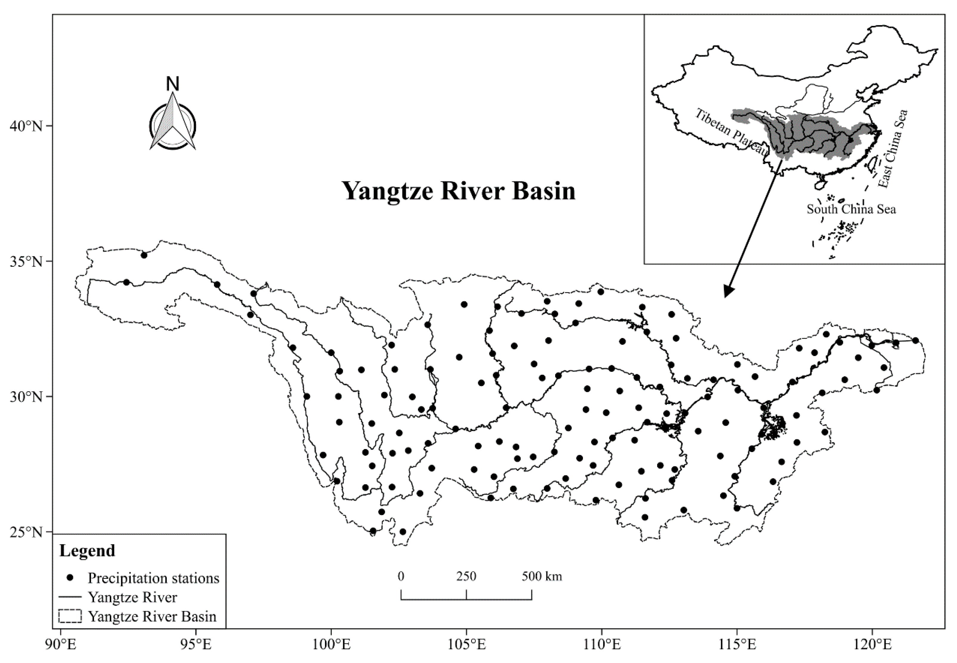
The Yangtze River (also known as Changjiang) is the longest river in China, extending from the Tibetan Plateau to the East China Sea, about 6300 km long (Figure 1). Its drainage area occupied one-fifth of China with one-third of the country’s population. The basin climate is characterized by complex patterns of precipitation and subject to periodic flood and drought events throughout history [1,2]. Precipitation variability both in space and time can impact the uneven distribution of water resources [3], and the induced extreme events have caused severe economic losses and casualties [1,4,5]. For instances, 4,970,000 houses were flattened by the flood in 1998 occurring over the whole basin [6]. In addition, drought-flood abrupt alteration and continuous droughts that cross seasons are increasingly frequent over the Yangtze River Basin. The Chongqing city, which experienced a once-in-a-century drought in 2006, was hit by torrential rain in 2007. Consequently, analyzing the spatiotemporal variability of extreme precipitation events in the Yangtze River Basin is highly important.
Many studies have investigated the characteristics of seasonal precipitation over the basin. Gemmer et al. [7] demonstrated that during the period of 1960–2004, the precipitation increased significantly in the lower Yangtze region in summer, while a statistically significant negative trend was found in September at the middle reach. The floods in July tend to be increasing in the lower reach, and drought events occurring in May, September, and October are more frequent in the middle reach. Jiang et al. [8] illustrated the changes in the monthly precipitation in spring and summer, and the precipitation from April to August can impose a direct influence on seasonal flood hazards. The above-average summer precipitation leads to more floods, and less autumn precipitation could result in more droughts [9].
In addition to the inter-annual and intra-annual trend analyses, an increasing concern regarding climate modes has been aroused. The relationships between precipitation over East Asia and large-scale climate patterns, such as the El Niño Southern Oscillation (ENSO), North Atlantic Oscillation (NAO), Pacific Decadal Oscillation (PDO), and Atlantic Multi-decadal Oscillation (AMO), were identified through the influence of atmospheric circulation [10,11,12,13,14]. However, the underlying dynamics are various for these teleconnections of climate patterns and the seasonal precipitation. For examples, according to Xiao, Zhang and Singh’s [10] analysis, a negative PDO event can result in an increasing tendency of the spring precipitation over the Southwestern Yangtze River Basin, while the preceding positive ENSO events typically lead to a high intensity of precipitation in spring over the eastern basin. Therefore, these various physic-based climate patterns may aggravate extreme events in different regions and seasons. Understanding the conditions that lead to the extreme and rare precipitation events is of great importance.
Due to the large size of this basin (spanning more than 30° of longitude and 10° of latitude) and complex terrains (with elevation ranging from more than 5000 m at the region source to sea level at the estuary), the spatiotemporal variability of precipitation is important for analyses of extremes. Here, we used archetypal analysis (AA) to identify the spatiotemporal structure of seasonal extreme precipitation, similar to Steinschneider and Lall’s [15] analysis. Unlike the principle component analysis (PCA), which is typically used for dimension reduction and analysis of the spatiotemporal variability of hydrological variables based on principle components through orthogonal transformation [16], AA represents an individual in a dataset as a convex combination of pure patterns (i.e., archetypes) or, equivalently, the extremal points. Archetypal patterns represent a set of extremal points, thus making AA widely used for extreme event analysis. The decomposed archetypes are restricted to be a mixture of actual observations, which can ease their physical interpretability. AA has also been widely expanded into data analysis in many scientific research fields [17,18,19,20].
In order to analyze the spatiotemporal variability of seasonal extreme precipitation and the physical mechanisms that how the climate patterns influence the extreme precipitation, we seek to use the archetypal analysis to extract the extreme modes. The seasonal extreme modes will be used to address the following objectives:
- (1)
- Analyze the spatiotemporal variability of extreme season-scale precipitation through the AA, and perform the trend analysis of the archetype occurrence;
- (2)
- Identify the most variable seasonal precipitation that more archetypes dominate; and
- (3)
- Discuss the underlying physical mechanisms of how the climate patterns influence the variability of the extreme precipitation.
2. Data Sources
The daily precipitation with less than 5% missing data at 136 precipitation stations (Figure 1) over the entire Yangtze River Basin were obtained from China Meteorological Data Service Center (CMDC) [21] to perform the seasonal extreme precipitation variability at the basin-scale. The data period is from 1960 to 2014. The missing values at each specific precipitation station were interpolated by the average value of the two closest stations without missing values. The seasons are defined as following: winter from December to February; spring from March to May; summer from June to August, and autumn from September to November. Note that in the following, seasonal precipitation denotes the sum of daily precipitation in one season, while the seasonal extreme precipitation and extremal modes are the decomposed archetypes through the archetypal analysis (see next Section 3.1).
The relationships between the seasonal extreme precipitation over the Yangtze River Basin and modes of large-scale teleconnection patterns were investigated, including El Niño Southern Oscillation (ENSO) derived from the Extended Reconstructed Sea Surface Temperature (ERSST) version 4 [22], North Atlantic Oscillation (NAO), Summer North Atlantic Oscillation (SNAO) [23], Atlantic Multi-decadal Oscillation (AMO) [24], Arctic Oscillation (AO) derived from the sea-level pressure, Pacific Decadal Oscillation (PDO) [25]. Three-month moving averages were applied to the climate variables. All the climate datasets used in this study can be accessed from the KNMI Climate Explorer [26].
3. Methodology
3.1. Spatiotemporal Modes of Seasonal Extreme Precipitation
The archetypal analysis (AA) was applied here to extract the extremely spatiotemporal modes of seasonal precipitation over the Yangtze River Basin. Through the AA, each time-based observation can be represented as a convex combination of a limited number of archetypes, and each archetype is restricted to be mixtures of the original data [27,28,29]. The archetypes can be interpreted as a “pure type” of actual values, or be characterized as extremal spatial patterns (i.e., the data points on the boundary of convex hull of the data set). Stone and Cutler [28] showed that AA is better than the PCA at analyzing the extreme events that are infrequent. Steinschneider and Lall [15] also demonstrated the advantages through its application in investigating spatiotemporal variability of summer daily precipitation over the Eastern United States.
The AA decomposes the dataset in a similar way as the PCA, but with different underlying constraints to find the best approximations to the observations. Given an m × n matrix , where n is the number of observations and m is the number of precipitation stations, there exists p m-dimensional vectors , , … under the following constraints (Equations (1) and (2)), such that the mean squared error , with angle bracket denoting the mean, is minimized:
where the n vector contains the convex weights for the k-th archetype across all observations. The decomposed archetype is characterized as “archetypal patterns” of observations, and represents the seasonal extreme precipitation. is the approximation to the observation . The can be considered as a time series of coefficients, which is a projection of the data X onto the k-th archetype , in the same way to PC scores in PCA. It is also referred to as the mixture coefficients. The archetypes are convex combinations of the data X when p > 1 and, thus, the archetypes are either actual observations or convex mixtures of the observations [27]. Here, to perform the trend analysis and clearly present the result in Section 3.2, we firstly define the archetype that represents the event with minimum precipitation as null archetype and assign it with [15].
Cutler and Breiman [27] noted that vectors are not orthonormal and have no natural nesting structure, which is different from the PCA. This means that if one changes the p to p + 1, the archetypes are not necessarily the same as those identified previously. The p for data X in AA should be optimized to minimize the , with , , where RSS is the residual sum of square errors and is the spectral norm.
3.2. Trend Analysis of the Archetype Occurrence
To explore the seasonal variations and inter-annual trend of the archetypes, we defined the matrix A of mixture coefficients rather than B as the temporal variability of archetypal patterns of the seasonal precipitation [15]. Although the matrix B also contains the time series of length n, it describes which day is characterized best by one particular pure archetypal pattern. Thus, the time series of the k-th column of B may miss the day when an archetype is active if another archetype is also active, and does not represent how dominant each archetype is in any given days.
We focused our interest on which archetype is the dominant one in a season during 1960–2014. Each season was firstly categorized as being dominated by one single, discrete archetype, rather than being featured by a series of that represents the relative strength of the k-th archetype in the i-th season. According to Steinschneider and Lall's [15] analysis, even if in one season when there is an archetype being active, for the null archetype may still be very large. Hence, the values of with are compared in one season across the k archetypes, excluding the null archetype which has a minimum value of total precipitation in that season. In this study, we selected the threshold of 0.4 for , similar to that in Steinschneider and Lall’s [15] analysis, to ensure that the archetype is indeed active. While in the case that none of the archetypes can reach this line, we assigned the null archetype to that season as a dominant one. Consequently, we can identify the season in which more archetypes dominate the precipitation, indicating high temporal variability of the extreme precipitation modes.
In order to visualize the trend of the dominant archetype for each season across years, we applied a smoothing method, which is termed as locally-weighted scatterplot smoothing, to produce a smoothly varying estimate [31]. For each discrete archetype in one season within one year, the probability of the occurrence was fitted using low-degree polynomial regression for the subset of data near this point. The smoothing model is fitted using weighted least squares, giving more weight to points near the point , whose response is being estimated, while giving less weight to points further away.
3.3. Climate Teleconnections to the Extreme Precipitation
The relationship between the decomposed archetypes and climate patterns was investigated to explore the physical mechanism of the climate-induced extremes. To identify the climate patterns that are significantly correlated with one archetype, we calculated the averages of seasonal coefficients within one year to represent the averaged extremes, and aggregated the climate indices into three-month averaged variables. The extremes of seasonal precipitation lag the climate patterns from one to twelve months.
The linear regression method was used to assess the relative importance of the explanatory variables (i.e., the identified climate patterns) for the target variables (i.e., archetypal patterns of seasonal extreme precipitation). The relative importance is defined as the quantification of an individual explanatory variable’s contribution to a target variable in the linear equation. For the uncorrelated explanatory variables, this is simply computed through the R2 from univariate regression, and the full model’s R2 is the sum of all univariate R2. Thus, each explanatory variable’s contribution is the ratio of univariate R2 to the full model’s R2 [32]. However, for the climate patterns, there is likely a high correlation among them, and this method should not work. Here, we applied an “LMG” method proposed by Lindeman et al. [33] (implemented with the R package “relaimpo” by Grömping [32]). This considers one individual explanatory variable’s effect while combining with the other variables. It allows the correlated explanatory variables to benefit from each other’s shares, and can be seen as a way to take care of the uncertainty of information regarding the true underlying structure. The approach is based on a sequential R2, but take cares of the dependence on orderings by averaging over orderings using simple unweighted averages. We would like to direct readers to [32] and therein for a detailed mathematical formulation.
The underlying physical dynamics of the variability of extreme precipitation are analyzed and discussed.
4. Results and Discussion
4.1. Archetypal Analysis of the Seasonal Precipitation
We firstly apply the AA to the centered and scaled observations.
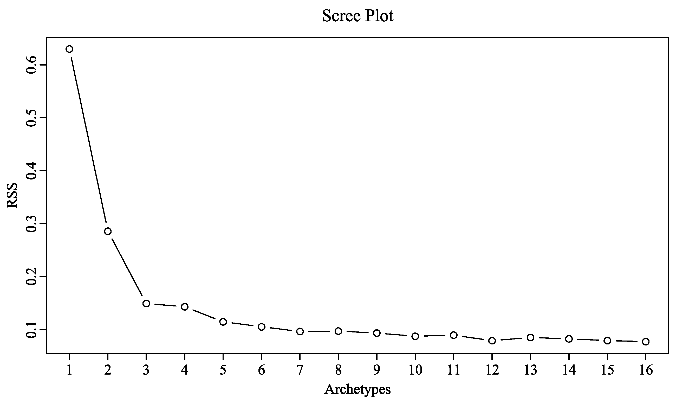
Figure 2 shows a scree plot that is used to select the appropriate number of archetypes to minimize the RSS to a sufficiently small level and be a global optimum. The curve shows a strong break at p = 3 and a weak break at p = 6. However, we would like to note that a relatively large number of archetypes are needed, suggesting the extreme precipitation is highly variable. Therefore, we will keep six archetypes to analyze the spatiotemporal variability of the seasonal extreme precipitation.
We present a simplex plot [34] (Figure 3) of the total average observed seasonal precipitation over the Yangtze River Basin to identify what precipitation that each archetype can represent. The stochastic nature of mixture coefficient implies that they exist on a standard p − 1 (i.e., 6 for p) simplex with p archetype as the corner, and coefficients as the coordinate with respect to these corners. These data were projected into two dimensions by a skew orthogonal transformation and all the vertices of the simplex plot are shown on a circle connected by edges. Observed precipitation with similar spatial patterns to one archetype will appear closer to the corresponding vertex. This plot provides a visual measure of the frequency of each archetype. The archetypes are notated as Ak for the k-th archetypal pattern.
Due to there being no natural orderings to the archetypes, we artificially assign the p (i.e., 6) to the archetype with smallest values and termed as the null archetype (i.e., A6). It is associated with dry air conditions or the East Asia winter monsoon with less water vapor [35]. The data points close to one vertex denote that the corresponding archetype dominates the spatial pattern on that day over the entire basin. We can find that the data points around A5 are more concentrated while, along with a wide range of values, suggesting that this seasonal extreme precipitation pattern is temporally more variable compared to others. The data concentration is possibly due to the observed precipitation being derived from the same climate events or occurring in the same season. A4 is the archetypal pattern with the least number of data points, but with the largest value of 671 mm, denoting the particularly rare and extreme mode relating to the above average and intensive precipitation. Thus, this archetypal pattern tended to lead a flood event over the Yangtze River Basin which may cause very large economic losses and human causalities (e.g., the flood event in 1998 [5,6]). The precipitation around A1 and A2 is spread more evenly across the archetypes indicating the mostly common modes, which represent the median precipitation from regular climate events, such as seasonal monsoons without extremely serious or persistent droughts. The relatively small precipitation shrinks to A3 and extends towards the null archetype A6.
The six spatial patterns for archetypes are shown in Figure 4 to highlight their similarities and differences. However, loadings for archetypes do not mean the relative weights of each archetype for the observations. This can be interpreted as how much each archetype contributes to the precipitation for each individual station.
A1 and A2 present the mostly common archetypes over the basin, and they exhibit a similar spatial pattern of extremes with closer values, even though in some parts they both show a small loading value. The central part of the A1 pattern and southeastern part of the A2 pattern show a weaker loading value than the other region. We can also see that the loadings of A4 are high across all stations over the Yangtze River Basin, which indicates that some large-scale extreme climate events have a wide influence on the whole basin (e.g., the continuous precipitation in the wet season over the region in 1998). On the other hand, A6 represents individuals which are small in loadings and associated with little total or no precipitation. This represents the whole basin was experiencing a period of dry conditions, such as a drought in East Asia relating to the La Niña events [2], and little total precipitation in winter [8]. A3 and A5 reflect the difference between the Western and Eastern Yangtze River Basin, but this difference is opposite for the two archetypes. A3 extends from the southeastern part with less precipitation to the northern part with large precipitation, while A5 dominates the southeastern basin with above-average precipitation, and westward with below-average precipitation. It is likely due to the southeastern part being impacted by the atmospheric circulation from the Pacific, while the western basin is subject to the monsoon from the Indian Ocean.
4.2. Trend Analysis of the Archetype Occurrence
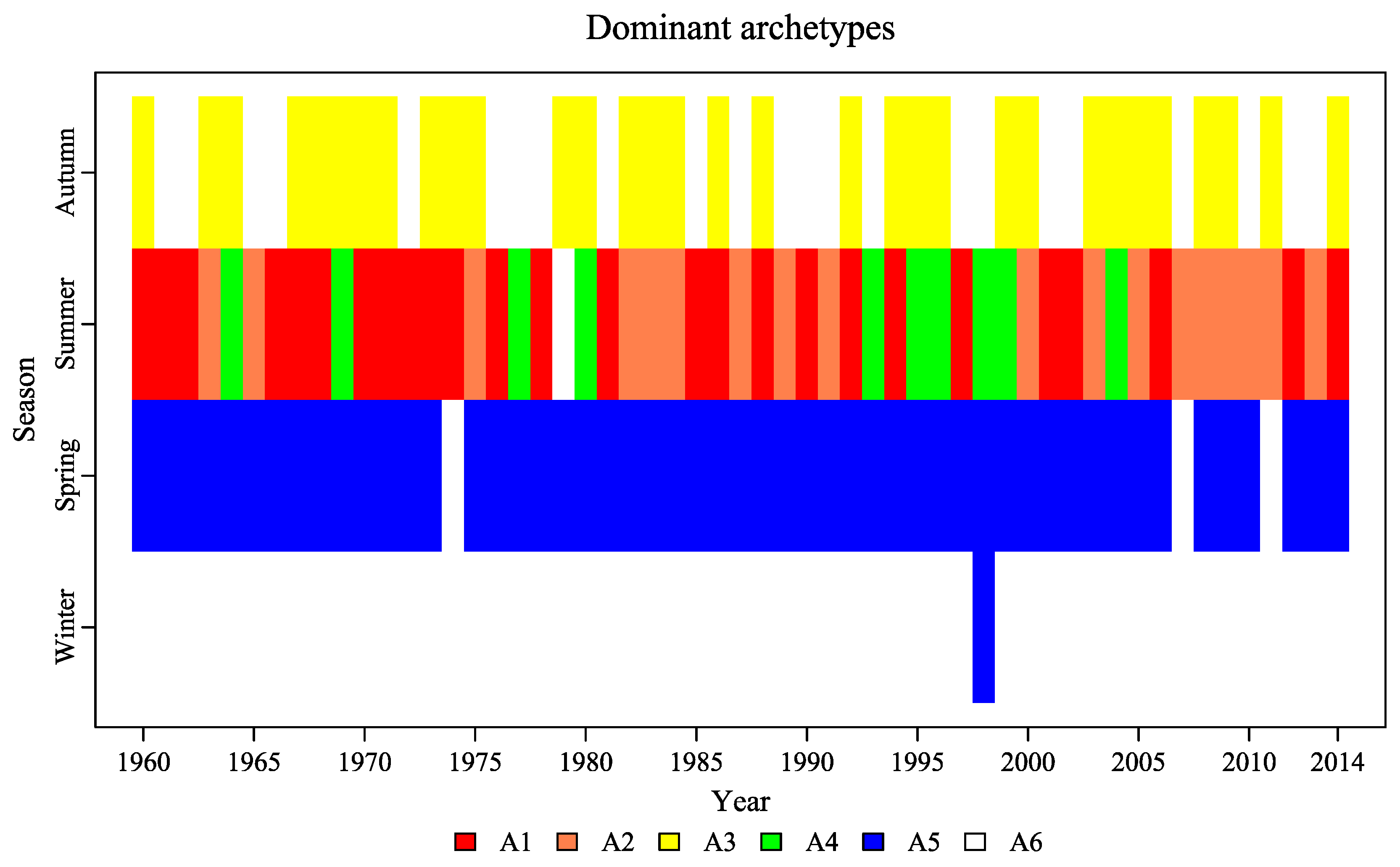
To explore the seasonal variations and inter-annual trend of archetypes, we show the dominant archetypes for each season within one year in Figure 5. The blank area in the figure denotes the null archetype associated with little total or no precipitation for that season. We can see that the winter is the mostly common season with null cases, except in 1998. This is due to the basin being dominated by the East Asia winter monsoon with less water vapor compared to other seasons [35]. During 1997–1998, the El Niño event had a lagged influence on the climate variability over the Yangtze River Basin, resulting in much more precipitation in winter [5,6,36]. The A5 prevails in spring during the whole period of 1960–2014. In the recent decade, because of the frequent occurrence of drought events (e.g., the years of 2007 and 2011 [37]), we can observe a couple of null archetypes. The periodic A6 and A3 dominate the below-average precipitation in autumn. In summary, the winter (A6-dry) and spring (A5-variable) consist almost entirely of a single archetype, and even autumn is made up of the two driest archetypes (A3 and A6), whereas summer precipitation can range from extremely dry (A6) to normal (A1 and A2) to extremely wet (A4). Thus, understanding what makes summer precipitation so variable is important.
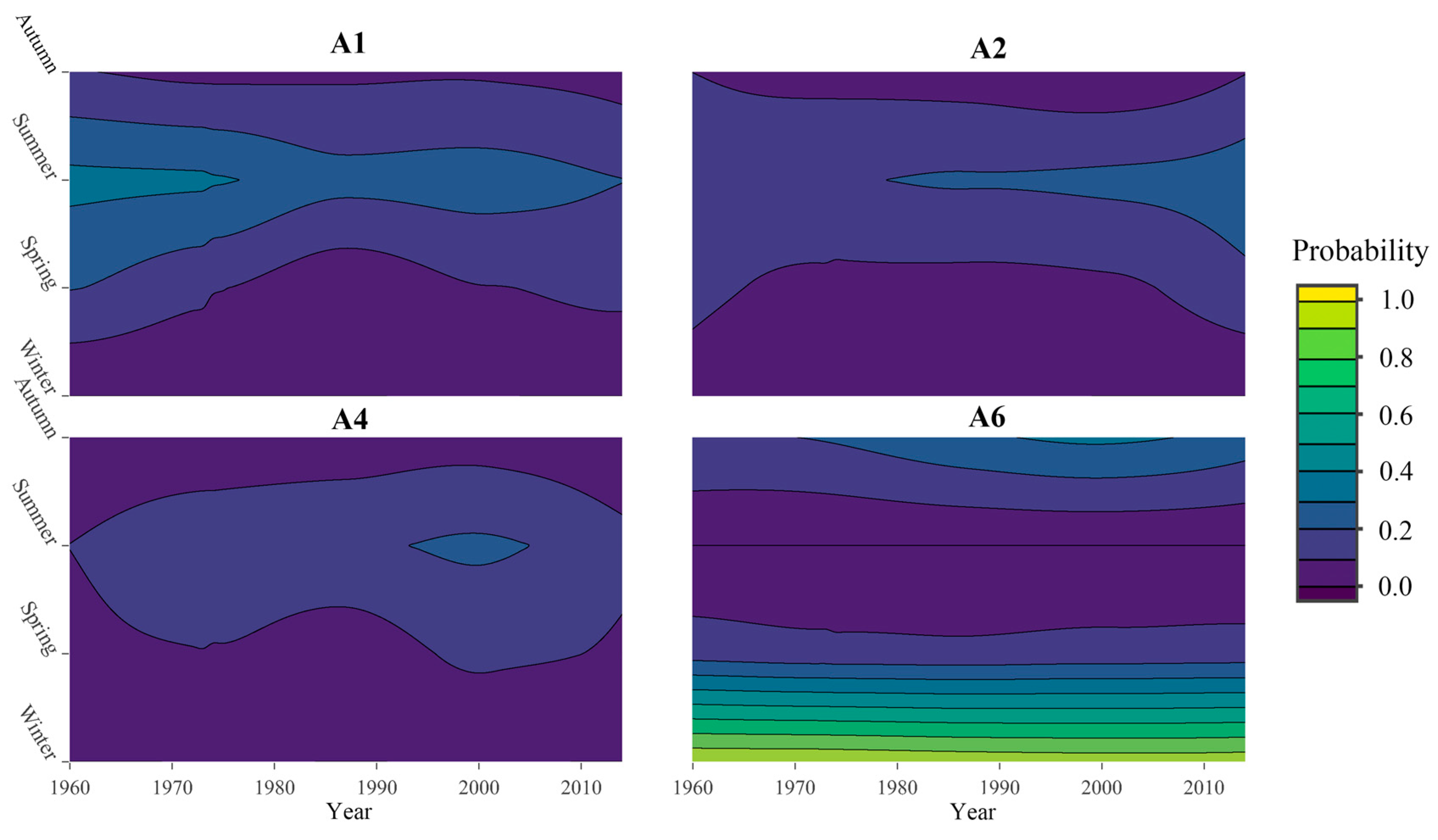
The probability of one discrete archetype occurrence in each season within one year is shown in Figure 6. Here, we focused on the frequency of the archetype occurrence in summer. A1 tended to be more frequent in summer before 1990, while A2 started to dominate the summer precipitation after 1990. This may be associated with the shift of the location of the El Niño developing phase from the Eastern Pacific to the Central Pacific since the early 1990s. Yu et al. [38] pointed out that the reason for this shift is possibly from the influence of AMO. A4 represents the events with particularly rare and extremely heavy precipitation in one season, which mainly occurred in the years around 2000 (e.g., the serious storm and flood in 1998 because of the infrequent El Niño occurrence [5,6,36]). The result is also consistent with the result of the dominant archetype analysis. A6 represents the events with below average or no precipitation, which are associated with the East Asia winter monsoon with the Siberian High bringing less moisture [35,39]. The precipitation falling in winter is far less than that in other seasons. Therefore, the probability of A6 occurrence is stable with a high value in winter during the whole period of 1960–2014.
4.3. Climate Teleconnections to the Archetypes of Summer Precipitation
We identified five climate patterns that were connected to the summer archetypes. Correlations of climate patterns and archetypes are shown in Table 1. For both A1 and A6, AMO shows positive correlations, while Niño4 is negatively correlated with them. Niño12 is negatively correlated with A1, while a strongly positive correlation with A4 was found, indicating Niño12 is likely to promote the occurrence of extremely heavy precipitation during summer. Niño3.4 is the only climate pattern that is significantly correlated with A2. In addition to Niño12 and Niño4 being positively correlated with the extremely wet pattern (A4), PDO is another large-scale climate pattern relating to the above-average precipitation.
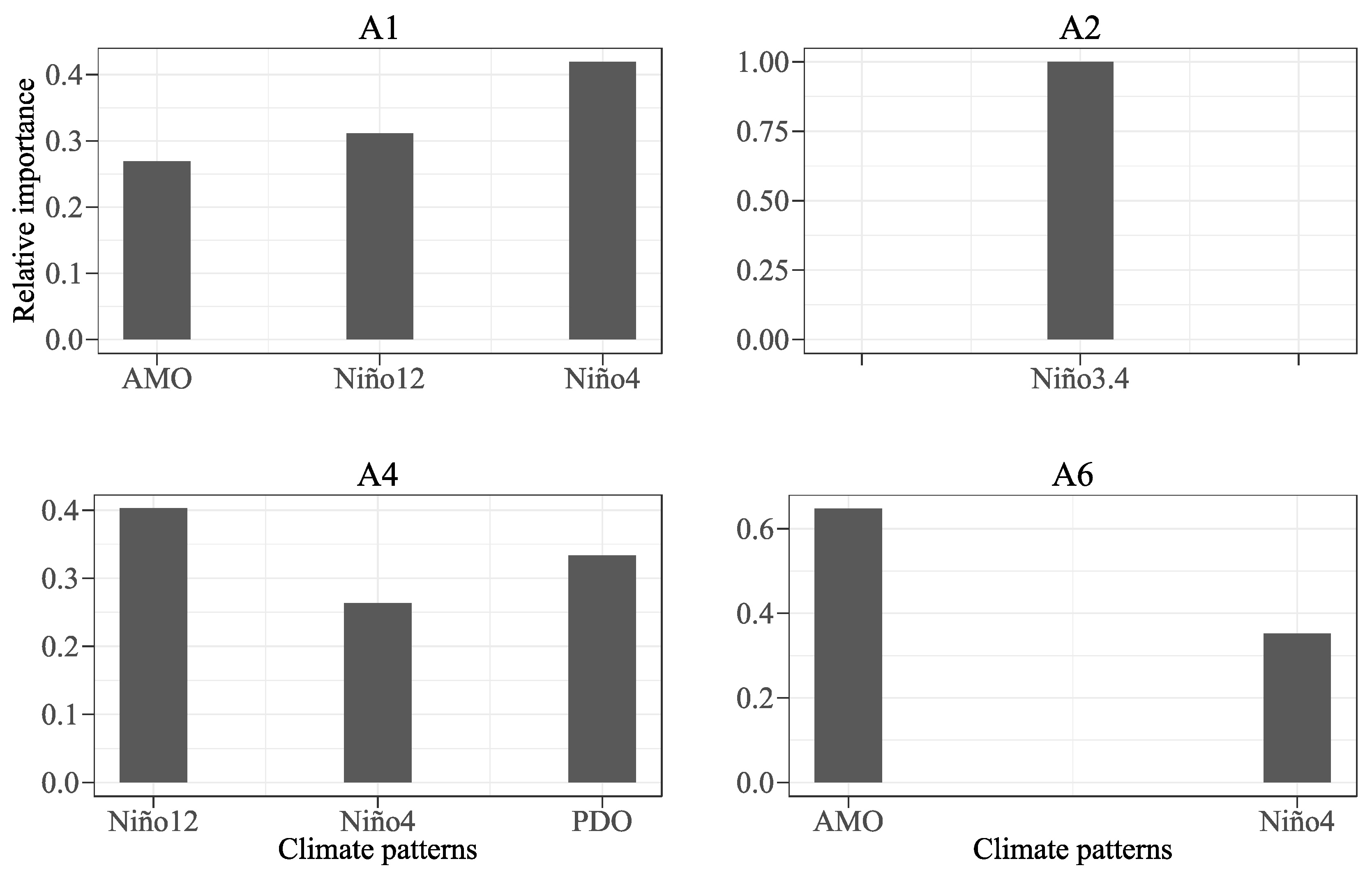
To quantitatively evaluate the relative importance of each climate pattern for the archetypes, we applied linear regression models to decompose the R2 into shares from the individual climate pattern. However, in the field of climate science, the indices are typically correlated. Therefore, we performed the further analysis considering these correlations to assess the relative importance, and presented the result in Figure 7.
The strongest determinant of the ensuing A1 is Niño4, which is consistent with the strong correlation of Niño4 and A1. Niño12 and AMO rank the second and third place, respectively. For the archetype A2, with which only one climate pattern was identified to be significantly correlated (i.e., Niño3.4), we consider Niño3.4 as the dominant driving factor with a value of 1.0 denoting the relative importance. For the archetype A4, we can see the largest contribution is from Niño12, which occurred in the Eastern Pacific Ocean and is associated with the ENSO events. For the null archetype A6, which represents the events with below-average precipitation, AMO contributes most to the droughts. In general, the ENSO indices including Niño12, Niño3.4, and Niño4 are connected to the archetypes representing the events with above average precipitation (e.g., A1, A2, and A4), while AMO can contribute much to the events with below average precipitation (e.g., A6).
4.4. Discussion of the Physical Mechanisms for Climate Teleconnections to the Extreme Precipitation during Summer
The identified AMO, which is defined by Schlesinger and Ramankutty [40], typically refers to multi-decadal variations of SST in the North Atlantic. Si and Ding [41] illustrated that a warm (cold) phase of AMO can usually cause the anomalous high (low) SST over the North Pacific center through AMO-Northern Hemisphere teleconnection, and this may induce a cold (warm) phase of pseudo-PDO, which leads to negative (positive) precipitation anomalies over the Yangtze River Basin. In addition, Qian et al. [42] demonstrated that China’s drought events tend to be more controlled by AMO than the condition in the Pacific Ocean, especially since the early 1990s, which is linked to the influence of global warming. Thus, the AMO should be considered as a strong determinant of events with below average precipitation over the Yangtze River Basin. This is consistent with our analysis result in Section 4.3 that AMO contributes much to the events with below average precipitation.
We also investigated the correlations of the summer archetypes and the four ENSO indices (Niño12, 3, 3.4, and 4, corresponding to different regions from the east to the west in the tropical Pacific) [43]. Niño3.4 is the most commonly used index to define the El Niño of a warm phase and La Niña events of a cold phase. The others are used to characterize the unique nature of each event. During the phase of El Niño events, the trade winds over the Pacific blow from east to west across the Central Pacific along the equator. Sea level falls in the Western Pacific and rises in the east as warm water flows eastward [43]. This phenomenon results in warmer sea surface temperature and moistens the overlying air, which may further alter the normal precipitation patterns. The dynamic for La Niña events is opposite to El Niño events. Jiang et al. [2] showed that over the middle and lower reaches of the Yangtze River Basin, floods are significantly correlated with the El Niño events, while droughts have a close relationship with the La Niña events. The relationships are reversed over the upper basin. Likewise, Guo et al. [44] note that the Niño3.4 sea surface temperature has a lagged influence on the variation in lakes in East Asia. Here, we can observe that different archetypes are correlated with various Niño indices, suggesting that the extremal patterns are induced by different characteristics of the ENSO events.
In the developing stage of El Niño events (i.e., the occurrence of abnormal SST in the Niño12 region), a precipitation belt extends into the Yangtze River Basin, resulting in much precipitation. However, in the decaying stage of El Niño events (i.e., the occurrence of abnormal SST in the Niño4 region), not as much precipitation as in developing stages emerges over the basin [45]. During the La Niña events, the scenarios of precipitation are expected to exhibit opposite anomalies. Chen [45] illustrated that the La Niña events are not influential on the East Asia monsoon as the El Niño events. It is also demonstrated that if the El Niño event develops in autumn and winter, the precipitation in the following summer tends to be greater over the basin (e.g., Niño12 for A4) while, if it develops in spring and summer, it tends to be less there (e.g., Niño4 for A1 with a negative correlation). This is consistent with our result that the ENSO events contribute much more to the archetypes which denote above-average precipitation.
Many studies have shown the relationship between the East Asia precipitation and PDO, demonstrating that the warm phase of PDO is helpful to lead the positive precipitation anomalies in East China for the period of the 1960s–2010s [41]. Related to PDO, the warmer sea surface temperature over the Northwest Pacific Ocean and offshore China likely reduces the land-sea thermal contrast between the Yangtze River Basin and the Pacific Ocean, eventually causing a weaker East Asian summer monsoon. However, a weaker summer monsoon typically results in positive precipitation anomalies over the Yangtze River Basin [46]. This is consistent with our result that a significant correlation of PDO and A4 was found.
5. Conclusions
This study examined the potential to use archetypal analysis to explore the spatiotemporal variability of seasonal extreme precipitation over the Yangtze River Basin. The associations of large-scale climate patterns with archetypes that dominate the summer precipitation were investigated and discussed. The main conclusions can be summarized as follows:
(1) The AA approach enables the observations to be convex combined with a limited set of archetypes and can be interpreted as “pure archetypes” or characteristic extremal spatial patterns. Six archetypes were identified in this study, and they denote the different season-scale precipitation events ranging from extremely dry (A6) to normal (A3, A5, A1, and A2) to extremely wet (A4). However, AA is not without problems, and there is no guarantee for the optimum number of archetypes to be found, hence, several iterations are chosen to run the algorithm to obtain a global optimum. Another is that the method of determining the appropriate number of archetypes is used by the non-interference based “elbow criterion” on the RSS curve, but this can give us a relatively reasonable number.
(2) The trend analysis showed that the winter (A6-dry) and spring (A5-variable) precipitation consist of almost entirely a single archetype. Even autumn precipitation is made up of the two driest archetypes (A3 and A6), whereas summer precipitation can range from extremely dry (A6) to normal (A1 and A2) to extremely wet (A4). The probability of the archetype occurrence revealed that A1 and A2 dominate the summer precipitation before and after 1990, respectively. The archetype A4 relating to the extremely much precipitation in one season mainly occurred around 2000, while A6 occurrence is stable with a high value in winter during the whole period of 1960–2014. This enables us to better understand the trend of future extreme precipitation events mixed by the archetypes.
(3) The climate teleconnections to archetypes of summer precipitation were investigated, and the relative importance of each climate pattern was analyzed. The results showed that five large-scale climate patterns were associated with the extreme modes of summer precipitation. ENSO indices including Niño12, Niño3.4, and Niño4 are connected to the archetypes that represent the events with above-average precipitation (e.g., Niño12 for A4), while AMO can contribute much to the events with below-average precipitation (e.g., AMO for A6). A warm phase of PDO is likely to lead the positive precipitation anomalies in summer.
Much research is directed towards a further analysis of the relationship between the spatiotemporal patterns of extreme precipitation and the flood/drought events over different parts of the Yangtze River Basin. In this paper, we used the archetypal analysis to extract the extremal patterns of seasonal precipitation, with the interesting application of discerning the underlying climate dynamics, and both intra-annual and inter-annual trends of dominant archetypes. Thus, the approach demonstrated here allows one to know well the spatiotemporal distribution of climate-induced variation of hydrological variables, such as the high flow and low flow in the Yangtze River, and discriminate the changes induced by the rare and extreme events.
Acknowledgments
We would like to sincerely thank the editors and reviewers who provided valuable comments. Particular thanks go to Scott Steinschneider for providing the guidelines of archetypal analysis and positive comments. We would also like to thank our colleagues working at Hohai University for reviewing the results. This work is funded by the National Key Research Projects (grant No. 2016YFC0402704), National Natural Science Foundation of China (grant No. 41371047) and the Special Fund of State Key Laboratory of Hydrology-Water Resources and Hydraulic Engineering (grant No. 1069-514031112). Support from the China Postdoctoral Science Foundation (grant No. 2016M601711), and the Jiangsu Planned Projects for Postdoctoral Research Funds (grant No. 1601027B) is appreciated.
Author Contributions
This research presented here was carried out in collaboration among all authors. Zhenkuan Su performed the data processing, conducted the research methods, analyzed the results, and wrote the manuscript together with the co-authors. All authors discussed the structure and comment on the manuscript at all stages.
Conflicts of Interest
The authors declare no conflict of interest.
References
- Zhang, L.X.; Zhou, T.J. Drought over East Asia: A Review. J. Clim. 2015, 28, 3375–3399. [Google Scholar] [CrossRef]
- Jiang, T.; Zhang, Q.; Zhu, D.M.; Wu, Y.J. Yangtze floods and droughts (China) and teleconnections with ENSO activities (1470–2003). Quat. Int. 2006, 144, 29–37. [Google Scholar] [CrossRef]
- Kripalani, R.H.; Kulkarni, A. Monsoon rainfall variations and teleconnections over South and East Asia. Int. J. Climatol. 2001, 21, 603–616. [Google Scholar] [CrossRef]
- Bing, L.F.; Shao, Q.Q.; Liu, J.Y. Runoff characteristics in flood and dry seasons based on wavelet analysis in the source regions of the Yangtze and Yellow rivers. J. Geogr. Sci. 2012, 22, 261–272. [Google Scholar] [CrossRef]
- Heng, L.; Xu, Z.K. The 1998 floods of the Yangtze river, China. Nat. Resour. 1999, 35, 14–21. [Google Scholar]
- Zong, Y.Q.; Chen, X.Q. The 1998 flood on the Yangtze, China. Nat. Hazards 2000, 22, 165–184. [Google Scholar] [CrossRef]
- Gemmer, M.; Jiang, T.; Su, B.; Kundzewicz, Z.W. Seasonal precipitation changes in the wet season and their influence on flood/drought hazards in the Yangtze River Basin, China. Quat. Int. 2008, 186, 12–21. [Google Scholar] [CrossRef]
- Jiang, T.; Kundzewicz, Z.W.; Su, B. Changes in monthly precipitation and flood hazard in the Yangtze River Basin, China. Int. J. Climatol. 2008, 28, 1471–1481. [Google Scholar] [CrossRef]
- Zhang, Z.; Zhang, J.; Sheng, R. The seasonal precipitation and floods/droughts in the Yangtze River Basin. J. Qingdao Technol. Univ. 2010, 31, 67–72. (In Chinese) [Google Scholar]
- Xiao, M.Z.; Zhang, Q.; Singh, V.P. Influences of ENSO, NAO, IOD and PDO on seasonal precipitation regimes in the Yangtze River basin, China. Int. J. Climatol. 2015, 35, 3556–3567. [Google Scholar] [CrossRef]
- Linderholm, H.W.; Seim, A.; Ou, T.H.; Jeong, J.H.; Liu, Y.; Wang, X.C.; Bao, G.; Folland, C. Exploring teleconnections between the summer NAO (SNAO) and climate in East Asia over the last four centuries—A tree-ring perspective. Dendrochronologia 2013, 31, 297–310. [Google Scholar] [CrossRef]
- Li, S.L.; Jing, Y.Y.; Luo, F.F. The potential connection between China surface air temperature and the Atlantic Multidecadal Oscillation (AMO) in the Pre-industrial Period. Sci. China Earth Sci. 2015, 58, 1814–1826. [Google Scholar] [CrossRef]
- Yuan, F.; Berndtsson, R.; Uvo, C.; Zhang, L.; Jiang, P. Summer precipitation prediction in the source region of the Yellow River using climate indices. Hydrol. Res. 2016, 47, 847–856. [Google Scholar] [CrossRef]
- Yuan, F.; Yasuda, H.; Berndtsson, R.; Uvo, C.B.; Zhang, L.; Hao, Z.; Wang, X. Regional sea surface temperatures explain spatial and temporal variation of summer precipitation in the source region of the Yellow River. Hydrol. Sci. J. 2016, 61, 1383–1394. [Google Scholar] [CrossRef]
- Steinschneider, S.; Lall, U. Daily precipitation and tropical moisture exports across the Eastern United States: An application of archetypal analysis to identify spatiotemporal structure. J. Clim. 2015, 28, 8585–8602. [Google Scholar] [CrossRef]
- Westra, S.; Brown, C.; Lall, U.; Sharma, A. Modeling multivariable hydrological series: Principal component analysis or independent component analysis? Water Resour. Res. 2007, 43. [Google Scholar] [CrossRef]
- Chan, B.H.P.; Mitchell, D.A.; Cram, L.E. Archetypal analysis of galaxy spectra. Mon. Not. R. Astron. Soc. 2003, 338, 790–795. [Google Scholar] [CrossRef]
- Marinetti, S.; Finesso, L.; Marsilio, E. Archetypes and principal components of an IR image sequence. Infrared Phys. Technol. 2007, 49, 272–276. [Google Scholar] [CrossRef]
- Eugster, M.J.A. Performance profiles based on archetypal athletes. Int. J. Perform. Anal. Sport 2012, 12, 166–187. [Google Scholar]
- Ragozini, G.; Palumbo, F.; D’Esposito, M.R. Archetypal analysis for data-driven prototype identification. Stat. Anal. Data Min. 2017, 10, 6–20. [Google Scholar] [CrossRef]
- China Meteorological Data Service Center (CMDC). Available online: http://data.cma.cn/en (accessed on 1 March 2017).
- Huang, B.Y.; Banzon, V.F.; Freeman, E.; Lawrimore, J.; Liu, W.; Peterson, T.C.; Smith, T.M.; Thorne, P.W.; Woodruff, S.D.; Zhang, H.M. Extended reconstructed sea surface temperature version 4 (ERSST.v4). Part I: Upgrades and intercomparisons. J. Clim. 2015, 28, 911–930. [Google Scholar] [CrossRef]
- Folland, C.K.; Knight, J.; Linderholm, H.W.; Fereday, D.; Ineson, S.; Hurrell, J.W. The summer north Atlantic oscillation: Past, present, and future. J. Clim. 2009, 22, 1082–1103. [Google Scholar] [CrossRef]
- Knight, J.R.; Folland, C.K.; Scaife, A.A. Climate impacts of the Atlantic Multidecadal Oscillation. Geophys. Res. Lett. 2006, 33. [Google Scholar] [CrossRef]
- Mantua, N.J.; Hare, S.R.; Zhang, Y.; Wallace, J.M.; Francis, R.C. A Pacific interdecadal climate oscillation with impacts on salmon production. Bull. Am. Meteorol. Soc. 1997, 78, 1069–1079. [Google Scholar] [CrossRef]
- KNMI Climate Explorer. Available online: https://climexp.knmi.nl/start.cgi?id=someone@somewhere (accessed on 1 March 2017).
- Cutler, A.; Breiman, L. Archetypal analysis. Technometrics 1994, 36, 338–347. [Google Scholar] [CrossRef]
- Stone, E.; Cutler, A. Introduction to archetypal analysis of spatio-temporal dynamics. Phys. D Nonlinear Phenom. 1996, 96, 110–131. [Google Scholar] [CrossRef]
- Eugster, M.J.A.; Leisch, F. Weighted and robust archetypal analysis. Comput. Stat. Data Anal. 2011, 55, 1215–1225. [Google Scholar] [CrossRef] [Green Version]
- Eugster, M.J.A.; Leisch, F. From spider-man to hero—Archetypal analysis in R. J. Stat. Softw. 2009, 30, 1–23. [Google Scholar] [CrossRef]
- Cleveland, W.S. Robust locally weighted regression and smoothing scatterplots. J. Am. Stat. Assoc. 1979, 74, 829–836. [Google Scholar] [CrossRef]
- Grömping, U. Relative importance for linear regression in R: The package relaimpo. J. Stat. Softw. 2006, 17. [Google Scholar] [CrossRef]
- Lindeman, R.H.; Gold, R.Z.; Merenda, P.F. Introduction to Bivariate and Multivariate Analysis; Scott Foresman: Glenview, IL, USA, 1980. [Google Scholar]
- Seth, S.; Eugster, M.J.A. Probabilistic archetypal analysis. Mach. Learn. 2016, 102, 85–113. [Google Scholar] [CrossRef]
- Chang, C.P.; Lu, M.M. Intraseasonal predictability of Siberian High and East Asian Winter Monsoon and its interdecadal variability. J. Clim. 2012, 25. [Google Scholar] [CrossRef]
- Cheng, M.H.; He, H.Z.; Mao, D.Y.; Qi, Y.J.; Cui, Z.H.; Zhou, F.X. Study of 1998 heavy rainfall over the Yangtze River Basin using TRMM data. Adv. Atmos. Sci. 2001, 18, 387–396. [Google Scholar] [CrossRef]
- Facts and Details. Available online: http://factsanddetails.com/china/cat10/sub64/item1879.html (accessed on 1 August 2017).
- Yu, J.Y.; Kao, P.K.; Paek, H.; Hsu, H.H.; Hung, C.W.; Lu, M.M.; An, S.I. Linking emergence of the Central Pacific El Niño to the Atlantic Multidecal Oscillation. J. Clim. 2014, 28, 651–662. [Google Scholar] [CrossRef]
- Zhang, Z.; Gong, D.; Hu, M.; Guo, D.; He, X.; Lei, Y. Anomalous winter temperature and precipitation events in southern China. J. Geogr. Sci. 2009, 19, 471–488. [Google Scholar] [CrossRef]
- Schlesinger, M.E.; Ramankutty, N. An oscillation in the global climate system of period 65–70 years. Nature 1994, 367, 723–726. [Google Scholar] [CrossRef]
- Si, D.; Ding, Y.H. Oceanic forcings of the interdecadal variability in East Asian summer rainfall. J. Clim. 2016, 29, 7633–7649. [Google Scholar] [CrossRef]
- Qian, C.C.; Yu, J.Y.; Chen, G. Decadal summer drought frequency in China: The increasing influence of the Atlantic multi-decadal oscillation. Environ. Res. Lett. 2014, 9. [Google Scholar] [CrossRef]
- Trenberth, K.; National Center for Atmospheric Research Staff (Eds.) The Climate Data Guide: Niño SST Indices (Niño 1 + 2, 3, 3.4, 4; ONI and TNI). Available online: https://climatedataguide.ucar.edu/climate-data/nino-sst-indices-nino-12–3-34–4-oni-and-tni (accessed on 1 August 2017).
- Guo, J.Y.; Sun, J.L.; Chang, X.T.; Guo, S.Y.; Liu, X. Correlation analysis of Niño3.4 SST and inland lake level variations monitored with satellite altimetry: Case studies of Lakes Hongze, Khanka, La-ang, Ulungur, Issyk-kul and Baikal. Terr. Atmos. Ocean. Sci. 2011, 22, 203–213. [Google Scholar] [CrossRef]
- Chen, W. Impacts of El Niño and La Niña on the cycle of the East Asian winter and summer monsoon. Chin. J. Atmos. Sci. 2002, 26, 595–610. (In Chinese) [Google Scholar]
- Wang, B.; Wu, Z.W.; Li, J.P.; Liu, J.; Chang, C.P.; Ding, Y.H.; Wu, G.X. How to measure the strength of the East Asian summer monsoon. J. Clim. 2008, 21, 4449–4463. [Google Scholar] [CrossRef]
Figure 1.
The spatial distribution of precipitation stations in the Yangtze River Basin used in this study.
Figure 1.
The spatial distribution of precipitation stations in the Yangtze River Basin used in this study.

Figure 2.
Scree plot of the result from AA. The maximum number of archetypes is initially set as 16 and eight chains were set to run to obtain a global optimum. We used the non-interference-based “elbow criterion” on the RSS curve to select the appropriate number of archetypes.
Figure 2.
Scree plot of the result from AA. The maximum number of archetypes is initially set as 16 and eight chains were set to run to obtain a global optimum. We used the non-interference-based “elbow criterion” on the RSS curve to select the appropriate number of archetypes.

Figure 3.
Simplex plot of seasonal precipitation with respect to the decomposed 6 archetypes. The data points are colored by the average observed precipitation over the whole Yangtze River Basin. The archetypes at the corners represent the extremal patterns, and are notated as Ak for the k-th archetypal pattern.
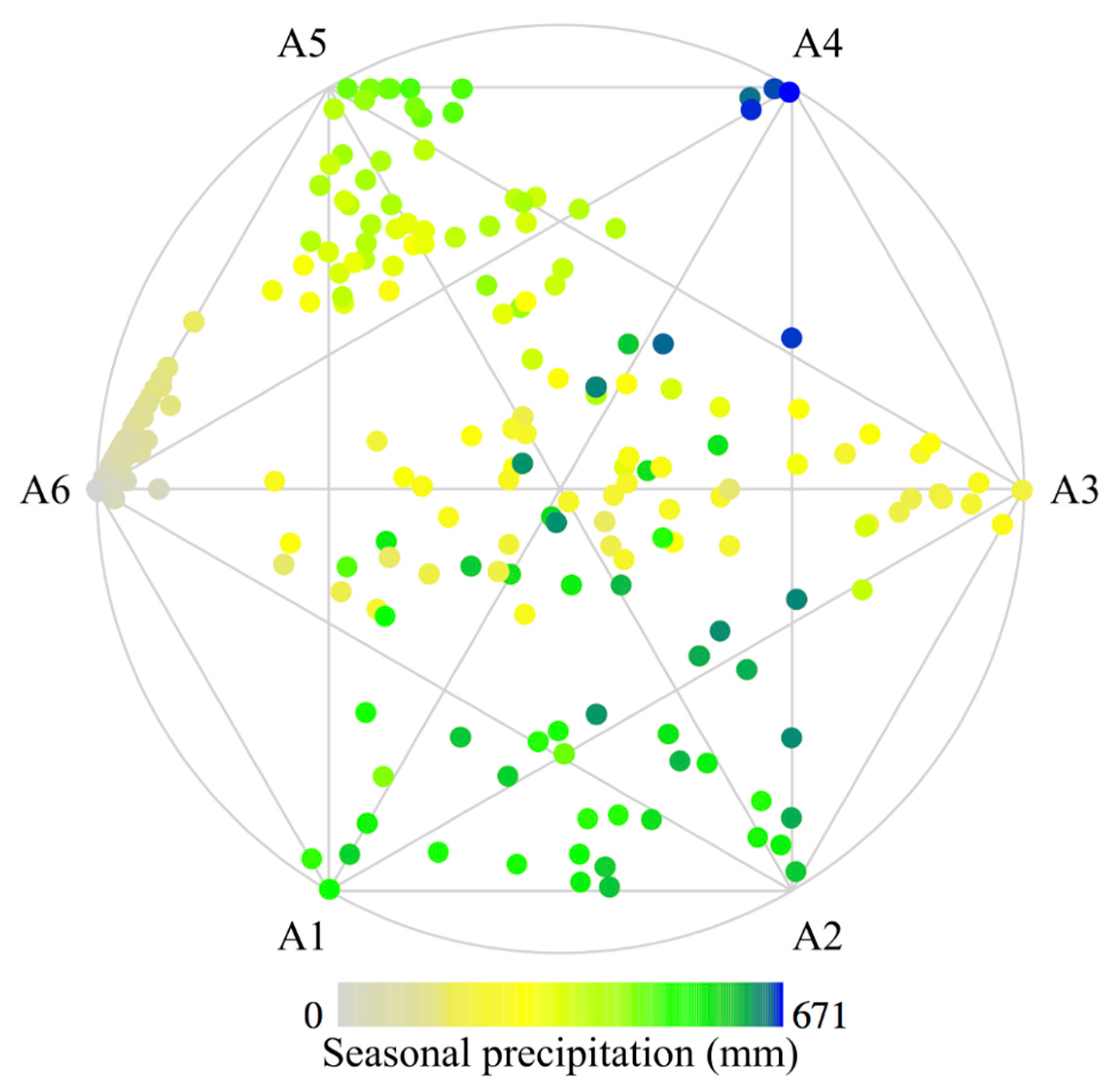
Figure 4.
Loading patterns of archetypes for seasonal extreme precipitation across stations over the Yangtze River Basin.
Figure 4.
Loading patterns of archetypes for seasonal extreme precipitation across stations over the Yangtze River Basin.
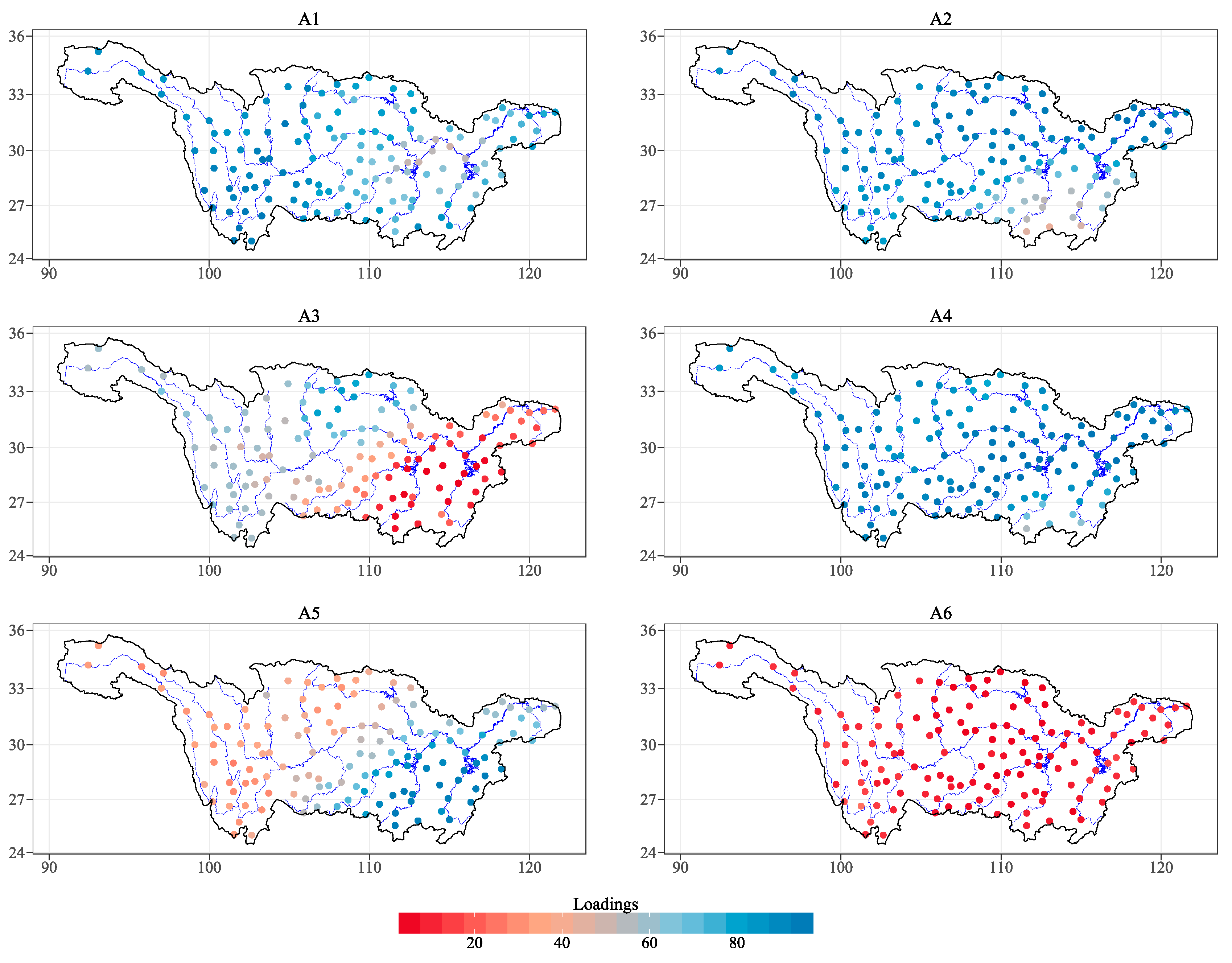
Figure 5.
Dominant archetypes for seasonal precipitation across years and seasons. The blank area in the figure represents the seasonal precipitation is dominated by the null archetype A6, relating to the events with little total or no precipitation for that season.
Figure 5.
Dominant archetypes for seasonal precipitation across years and seasons. The blank area in the figure represents the seasonal precipitation is dominated by the null archetype A6, relating to the events with little total or no precipitation for that season.

Figure 6.
Trends in probability of archetype occurrence for each season across years.

Figure 7.
Relative importance of the identified climate patterns for each archetype.


Table 1.
Correlations of the identified climate patterns and the summer archetypes at 95% confidence level. The time period of the archetypes is from 1960 to 2014 and the time period of the climate patterns is from 1959 to 2013. The season in the parentheses indicates the season for climate patterns with the strong correlation.
| Climate Patterns | A1 | A2 | A4 | A6 |
|---|---|---|---|---|
| AMO | 0.27 (July–September) | 0.37 (May–July) | ||
| Niño12 | −0.28 (November–January) | 0.34 (September–November) | ||
| Niño3.4 | −0.23 (May–July) | |||
| Niño4 | −0.32 (February–April) | 0.27 (February–April) | −0.30 (March–May) | |
| PDO | 0.33 (August–October) |
© 2017 by the authors. Licensee MDPI, Basel, Switzerland. This article is an open access article distributed under the terms and conditions of the Creative Commons Attribution (CC BY) license (http://creativecommons.org/licenses/by/4.0/).
Share and Cite
MDPI and ACS Style
Su, Z.; Hao, Z.; Yuan, F.; Chen, X.; Cao, Q. Spatiotemporal Variability of Extreme Summer Precipitation over the Yangtze River Basin and the Associations with Climate Patterns. Water 2017, 9, 873. https://doi.org/10.3390/w9110873
AMA Style
Su Z, Hao Z, Yuan F, Chen X, Cao Q. Spatiotemporal Variability of Extreme Summer Precipitation over the Yangtze River Basin and the Associations with Climate Patterns. Water. 2017; 9(11):873. https://doi.org/10.3390/w9110873
Chicago/Turabian StyleSu, Zhenkuan, Zhenchun Hao, Feifei Yuan, Xi Chen, and Qing Cao. 2017. "Spatiotemporal Variability of Extreme Summer Precipitation over the Yangtze River Basin and the Associations with Climate Patterns" Water 9, no. 11: 873. https://doi.org/10.3390/w9110873
Note that from the first issue of 2016, this journal uses article numbers instead of page numbers. See further details here.