Physical Experiment and Numerical Simulation of the Artificial Recharge Effect on Groundwater Reservoir
by
Yang Xu
, 
Longcang Shu
*,
Yongjie Zhang
,
Peipeng Wu
,
Abunu Atlabachew Eshete
and
Esther Chifuniro Mabedi
State Key Laboratory of Hydrology-Water Resources and Hydraulic Engineering, Hohai University, Nanjing 210098, China
*
Author to whom correspondence should be addressed.
Water 2017, 9(12), 908; https://doi.org/10.3390/w9120908
Submission received: 4 October 2017
/
Revised: 17 November 2017
/
Accepted: 20 November 2017
/
Published: 23 November 2017
Abstract
:To improve the efficiency of utilizing water resources in arid areas, the mechanism of artificial recharge effecting on groundwater reservoir was analyzed in this research. Based on a generalized groundwater reservoir in a two-dimensional sand tank model, different scenarios of the infiltration basin location and recharge intensity are designed to study how to improve the efficiency of groundwater reservoir artificial recharge. The effective storage capacity and the effective storage rate are taken as the main parameters to analyze the relation between recharge water volume and storage capacity. By combining with groundwater flow system theory, FEFLOW (Finite Element subsurface FLOW system) is adopted to set up the groundwater numerical model. It is used to verify the experiment results and to make deep analysis on the rule of water table fluctuations and groundwater movement in the aquifer. Based on the model, different scenarios are designed to examine the combined effect of recharge intensity and intermittent periods. The research results show that: the distance between infiltration basin and pumping well should be shortened appropriately, but not too close; increasing recharge intensity helps to enlarge the effective storage capacity, but it can also reduce the effective storage rate, which goes against the purpose of effective utilization of water resources; and, the recharge intensity and recharge duration should be given full consideration by the actual requirements when we take the approach of intermittent recharge to make a reasonable choice.
1. Introduction
In arid/semi arid regions, surface water resources are generally scarce and highly unreliable, so groundwater is the primary water source in these regions [1]. However, groundwater in these areas is mainly fossil water and is not sustainable [2] to meet human and ecosystem needs. Therefore, some artificial measures are needed to sustainable manage the aquifers. The construction of groundwater reservoir plays an important role in improving water resources utilization and ensuring water supply safety [3]. Groundwater reservoir is a popular water resources management method in China [4], which is similar to the concept of aquifer storage and recovery [5,6,7] in America. When compared with surface reservoirs, groundwater reservoirs have many advantages in no occupation of land, no immigration, less evaporation, and a simple structure. Nowadays, groundwater reservoir are used in three ways: (1) Conjunctive use of surface water and groundwater to augment groundwater resources [8]; (2) Recovering the cone of depression formed by over-exploitation of groundwater [9]; and, (3) alleviating land subsidence [10], soil erosion, and seawater intrusion, and other typical geo-hazards in coastal areas [11,12]. To solve the problem of regulation and storage of water resources, one of the key construction techniques is the diversion of infiltration system.
In previous studies, Thompson [13] discussed the efficiency of the recharge by analyzing the variations on water-table mounding during the recharge experiments by storm water infiltration basins. It suggests that mound heights increased as the initial soil moisture, infiltration basin area, and ponding depth rose. Nimmer’s study [14] shows that the groundwater level height increased as the thickness of unsaturated zone decreased with the same infiltration conditions. However, less of the research of artificial recharge system concentrated on the combined effects of artificial recharge and exploitation, which plays an important role in water resources regulation of groundwater reservoir. Moreover, the exploitation disturbed the natural groundwater flow, and the hydraulic gradient is no more the only driving factor of the fluxion. It is unclear whether the research methods and results of artificial recharge is still valid in the groundwater reservoir, and most of the previous studies of the interaction between recharge and discharge are based on the large volume of hydrological data [15,16] (precipitation, surface runoff, evapotranspiration, change in groundwater storage, etc.). In fact, these long-time data accumulated over a considerable time period, which is inadequate or unreliable [17] in many areas. The complex geographical conditions [18] of the field study area will also limit the quantity and position of observation points in some literatures. An advantage of laboratory experiments for the artificial recharge system is that the requirements are often for shorter-term and more easily obtained data.
There are three main research methods were used to discuss the influences of artificial recharge. First, water budget analysis [19,20] is used to estimate inflow based on the law of conservation of mass. Second, water table fluctuation method [21,22,23] is a useful tool for determining the magnitude of both short-and long-term changes in groundwater recharge, and has been widely applied under varying climatic conditions. Third, tracer techniques [24] are widely used in arid and semi-arid to estimate groundwater recharge. However, the above methods do not measure water fluxion or quantity directly, which may cause an over- or under-estimation of recharge. Furthermore, with the development of computer technology, the numerical simulation method [2,25], which is based on water balance principle and Richard’s equation, has been widely used. In this paper, we applied and discussed three methods (the water table fluctuation method, water budget analysis, and numerical method).
The main objectives of this study are: (1) to evaluate the combined effects of artificial recharge and groundwater exploitation on pore water flow in groundwater reservoir; and, (2) to evaluate the temporal variability of groundwater circulation under the influencing of artificial recharge. Both laboratory experiments and corresponding numerical simulations were conducted to explore the efficiency of artificial recharge in groundwater level, under conditions of different distance and recharge intensity by infiltration basin, when the exploitation kept stabilization. The numerical model was also applied to calculate the water exchange between the aquifer and its boundary conditions. It was used to compare the effect of intermittent recharge under five regulation scenarios, based on the marked difference of the recharge water resource in different seasons. The purpose was to evaluate the influence of differential artificial recharge distance, intensity, and duration, and to increase the efficiency of artificial recharge in groundwater reservoir.
2. Physical Model
2.1. Experiment Setup
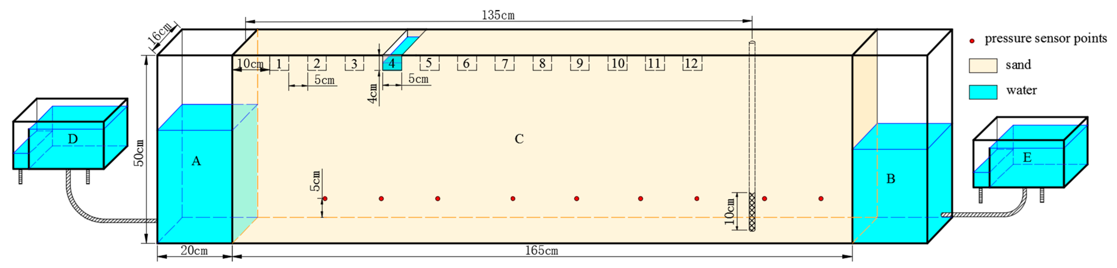
In order to generalize the complicated structure of the groundwater system, the experiment was designed to focus on flow processes in the horizontal and vertical directions. Experiments were conducted in a 205 cm (long) × 50 cm (high) × 16 cm (wide) tank (Figure 1), which was built by the colorless plexiglass with 10 mm thickness. The tank was divided into three chambers by the plexiglass screens, which are located 20 cm away from both ends of the tank. The plexiglass screens were covered with fine stainless steel mesh to prevent sand migration and to ensure the water fluxion to other chambers. The left (A) and right (B) chambers were used to maintain constant heads of the middle chamber (C) and their water levels can be controlled through the adjustable water boxes (D and E), which simulate the natural groundwater hydraulic gradient and water cycle process. The middle chamber (C) was filled with porous medium; it was packed with uniform, homogenous sand. Thus, the range of the experimental aquifer is 165 cm long, 16 cm wide, and 50 cm high. During packing, the sand was fully compacted to minimize consolidation and air entrapment [26]. Every layer of the medium was limited to 5 cm. The water level was raised after packing every 5 cm and the process was repeated until the entire tank was packed. Particle size distribution of the sand was analyzed by using laser diffraction particle size analyzer apparatus. The results (Table 1, Figure 2) indicated that the sand is homogenous medium to coarse sand. Thus, the sand tank system can be regarded as a homogeneous isotropic porous aquifer. A partial penetrating pumping well was used to simulate groundwater exploitation. The pumping well was made of polyvinyl chloride (PVC) pipe with an internal diameter of 1.5 cm, and was partially screened at bottom 10 cm. It was located 135 cm away from the left side of the middle chamber. A peristaltic pump that was connected to the pumping well by tube to ensure the groundwater can be pumped out at constant rate from aquifer. An infiltration basin was made by a 5 cm (long) × 4 cm (high) × 16 cm (wide) plastic box, which was buried in 4 cm deep of the sand tank. The top of the infiltration basin was connected with another peristaltic pump to simulate artificial recharge and the bottom of the infiltration basin is permeable. The position of the infiltration basin was determined according to the experimental scenarios. Over the back of the tank, nine pressure sensor points (red points shown in Figure 1) are distributed to record real-time data of the groundwater level. The hydraulic conductivity of the aquifer was 40.61 m/day and the specific yield was 0.13, as measured by a pumping test before the experiment.
Both sides of the water level were set by adjusting the height of the constant head containers. The up-stream is on the left and is controlled at 30 cm, while the down-stream is on the right and is controlled at 25 cm. The pumping rate was 1 mL/s and the corresponding unit-width pumping rate was 6 mL/s·m. After about 2 h continual exploration, the groundwater flow system reached a relatively steady state. The groundwater level was dropping sustainably, and then formed an obvious cone of depression. This experiment can represent the groundwater artificial pumping process. This experiment focus on X and Y directions, so that the pumping rate and infiltration intensity have turned into unit width flux rate on a vertical section. Finally, a groundwater artificial exploitation system was established. During the experiment, artificial recharge system was the main study subject in the groundwater flow system. 12 different recharge positions were chosen (position 1, position 2,…, position 12) to study. They are located from 10 cm to 130 cm from the left side every 5 cm (shown in Figure 1). Moving the position of the infiltration basin in corresponding scenarios to ensure that it can be evenly recharged by peristaltic pump. Theoretically, the infiltration intensity has no relationship with the pumping rate. Mostly, the infiltration rate is less than the pumping rate. The final selection of infiltration intensity is 2.4 mL/s·m, 3.6 mL/s·m, 4.8 mL/s·m, 6 mL/s·m, and 7.2 mL/s·m. When the infiltration intensity is 7.2 mL/s·m, it reaches the maximum infiltration capacity. No water spilled from the top or side of the infiltration basin to ensure that all of the recharge water can enter the aquifer. The groundwater level at corresponding positions in the sand tank were collected every 30 s through the pressure sensors until the groundwater level becomes steady. The real-time groundwater level was recorded in 60 scenarios, with 12 different recharge positions and five different recharge intensities.
2.2. Experimental Method
The artificial recharge to groundwater will increase the groundwater level and alter the water exchange between aquifer and boundaries. With the built groundwater reservoirs, more water can be collected from infiltration basin where it infiltrates into the soil and moves down to the groundwater. It can cause the drastic fluctuation of groundwater level. The groundwater level can be divided into two parts: the left part is an infiltration basin centric groundwater mound and the right part is a pumping well centric cone of depression. When the groundwater level of groundwater reservoir is higher than the groundwater level of the constant head boundary, the boundary will convert from inflow boundary to outflow boundary. The inflow water could be estimated by the specific yield and groundwater level from the beginning to the end of the experiment process. As it is mentioned in the research of Du in Shijiazhuang city [19], the volume of water that can be stored in groundwater reservoir is defined as the effective stored water, or effective storage capacity (ESC). The ratio of ESC to the volume of recharge water is defined as the effective storage rates (ESR). In this research, the concepts of the ESC and ESR are also used to quantify the effect of artificial recharge. When the infiltration intensity is constant, higher ESR leads to a faster change of water storage capacity and a better recharge result. However, when the volume of recharge is constant, higher ESC causes more water stored in the aquifer and better regulation plan.
Based on the above principles, the ESC is determined by the specific yield and the difference between initial and instant groundwater levels. Thus, as it is mentioned in Du’s study [19], the ESC (Qs) and the ESR (β) in time t can be obtained from the following equations:
where Qs(t) is the ESC of the groundwater reservoir; Sy is the specific yield of the aquifer; V*(t) is the groundwater storage variation volume; β(t) is the effective storage rate; and, Qr(t) is the quantity of artificial recharge.
In this study, the groundwater reservoir was generalized into a two-dimensional homogeneous isotropic unconfined aquifer in a laboratory scale. Because the groundwater levels (ht) are different in every point, it is difficult to calculate the difference between instant and initial groundwater level directly. Using the calculus equation (Equation (3)), which was developed by Equation (1) and Equation (2), can simplify the process of calculating the groundwater storage variation volume (V*) in the aquifer. V* is equal to the area surrounded by the groundwater levels in 0 and t s, which can be easily measured (Figure 3).
where l is the length of the sand tank; x is the distance apart from the left side; h0 is initial groundwater level, h0 = f0(x); ht is groundwater level after artificial recharge for t seconds, ht = ft(x); and, A (t) is the area surrounded by the groundwater levels in 0 and t s.
2.3. Experimental Results
2.3.1. Effect of Relative Distance between Infiltration Basin and Pumping Well
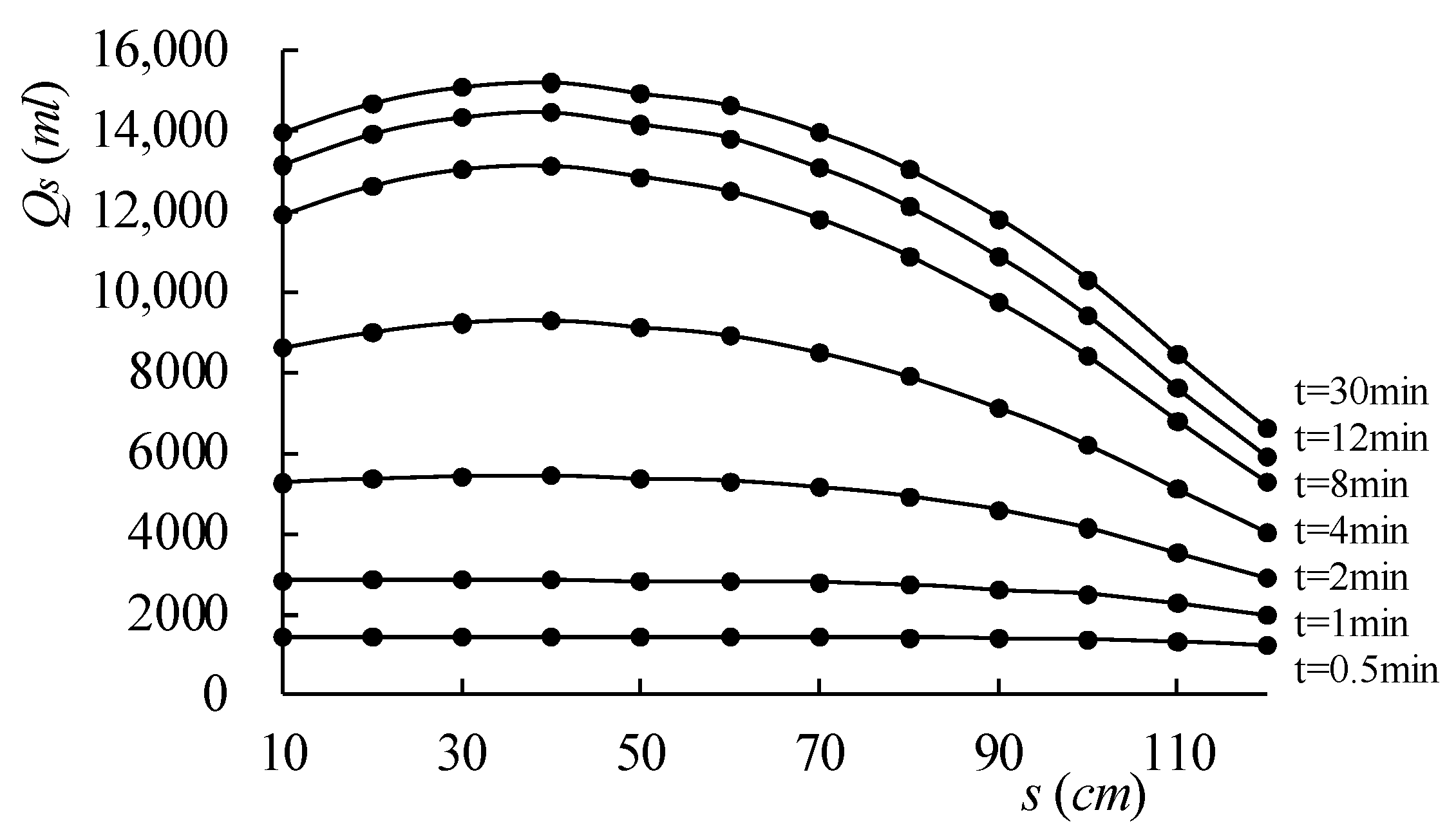
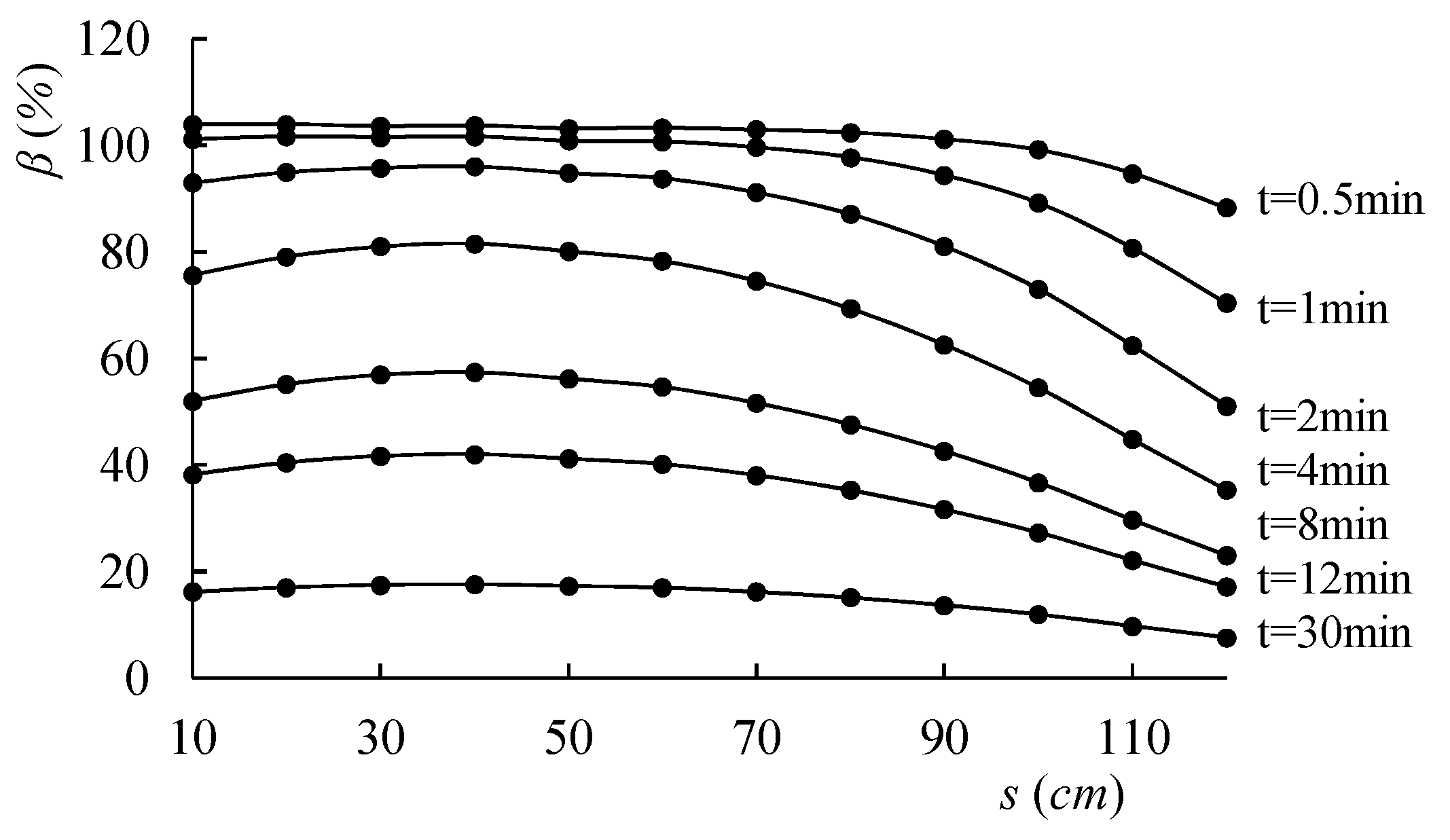
Assuming that the infiltration intensity is constant, the variation of relative horizontal distance between infiltration basin and pumping well has a different impact on the groundwater mound. The experimental distance was ranged from 10 cm to 120 cm according to 12 different positions of infiltration basin (shown in Figure 1). The ESC and the ESR in each moment can be calculated from the groundwater level data of the experiments. Taking the scenarios with the recharge intensity of 4.8 mL/s as an example, the ESC and the ESR were accounted at different moments, respectively. The ESC (Qs)—distance (s) relationship curves and the ESR (β)—distance (s) relationship curves were shown in Figure 4 and Figure 5.
As it shown in Figure 4 and Figure 5, at the beginning of the artificial recharge, the ESC and the ESR change little with distance. The variation of distance does not lead to significant changes in the effect of artificial recharge. With the increasing artificial recharge time, the variation of distance occurs in connection with the artificial recharge effect. When the distance increases from 10 cm to 40 cm, the ESC and the ESR increase simultaneously. Because the artificial recharge process was impacted by the artificial exploitation in the pumping well. The infiltration basin and the pumping well are too close to store water in the aquifer. Most of the recharge water is captured by the pumping well directly. While choosing the location of a groundwater reservoir, which artificial recharge and recovery from the shallow zone without dam, appropriate enlarge the relative distance from infiltration basin to the pumping is helpful to increase the area of groundwater mound and to store more water. When the distance is 40 cm from the pumping well to infiltration basin, the relationship curves come to the maximum growth, which is the location having the best effect. When the distance continues to increase from 40 cm to 120 cm, the value and growth rate of the ESC and the ESR obviously decrease. For example, when the recharge time reaches 30 min, the ESC increases by 106.8% at position 6 rather than position 1. The increase in distance also causes the decrease of the ESR. After 30 min’s of constant artificial recharge, the groundwater flow reached steady state in each positions, and the ESC reached its maximum value, equal to the concept of maximum storage capacity of the groundwater reservoir. The maximum effective storage capacity and the distance were related in a quadratic function (Figure 4, t = 30 min).
Experimental results demonstrate that when varying the recharge intensity between 2.4 mL/s·m, 3.6 mL/s·m, 4.8 mL/s·m, 6 mL/s·m, and 7.2 mL/s·m, the effect on the ESC and distance is almost the same. The maximum storage capacity were fitted with the quadratic function, and the maximum storage capacity appears on 37.8 cm, 38.2 cm, 39.7 cm, 40.6 cm, and 40.8 cm, respectively. Therefore, if only the recharge position is considered, the range of distance from 10 cm to 70 cm which near the maximum storage capacity is accepted as the appropriate distance in this experimental condition. Moreover, taking into account the transport distance from the recharge source, position 6 is the best choice to build an infiltration basin. Because position 6, which is 70 cm far away from pumping well, is the closest position to the recharge water source in the chosen field.
2.3.2. Effect of Recharge Intensity
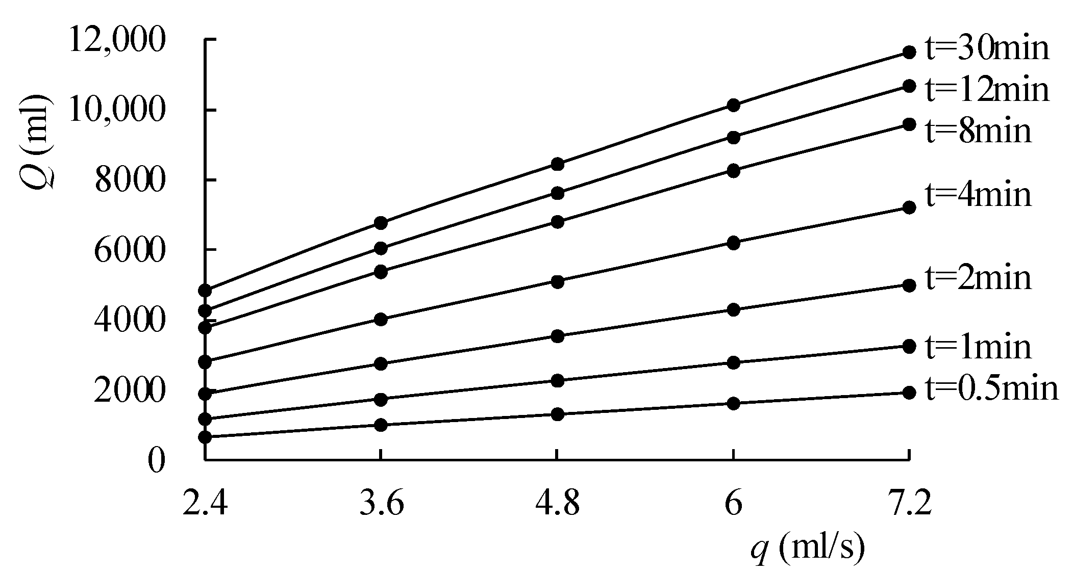
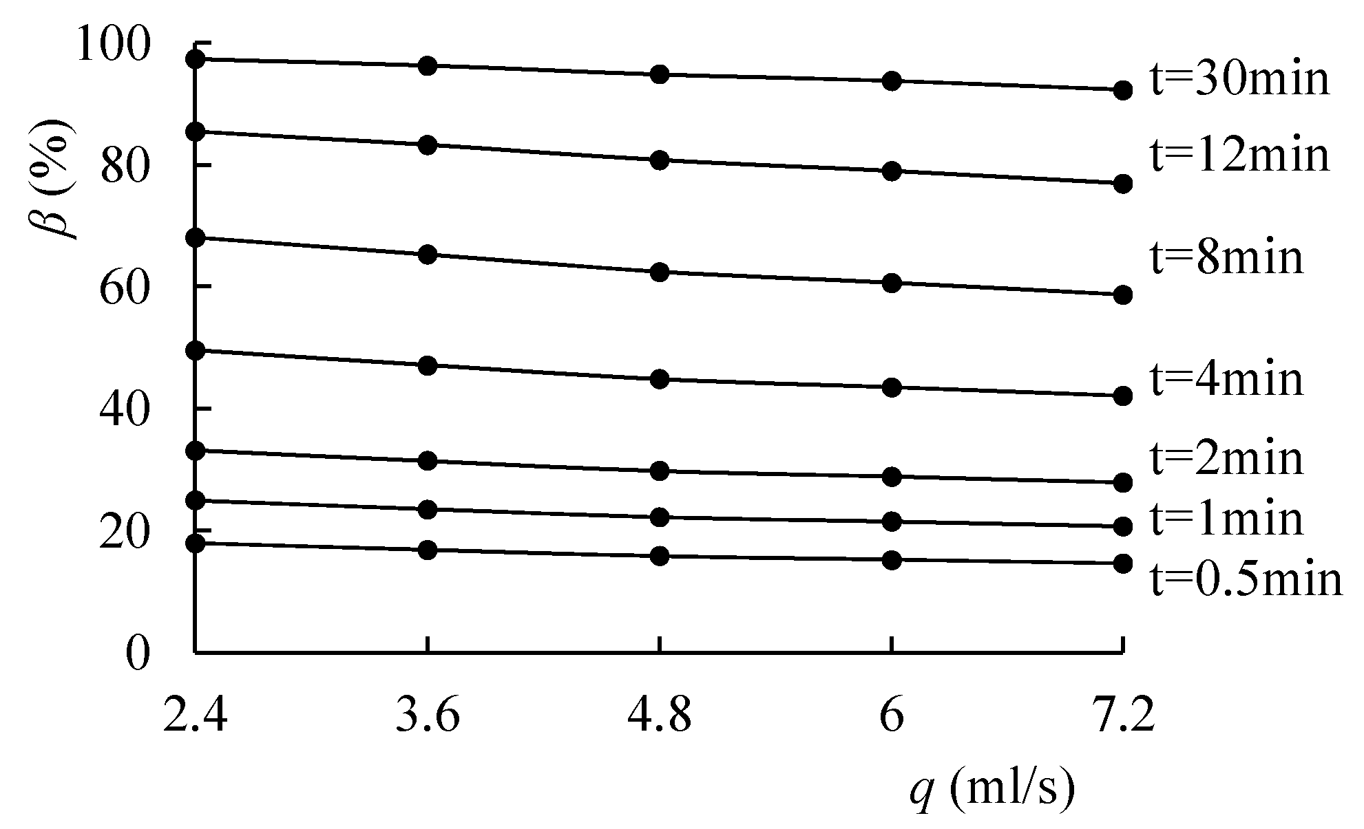
According to the experimental data of groundwater level, the ESC and ESR of different recharge intensities were calculated to analyze the influence of artificial recharge intensity on groundwater reservoir. Taking the experimental scenarios at position 2 as an example, the ESC (Qs)—recharge intensity, (q) relationship curves (Figure 6), and the ESR (β)—recharge intensity (q) relationship curves (Figure 7) in different time periods were drawn separately.
As shown in Figure 6, the larger the recharge is, the greater the SEC is in the same period. The relationship between the ESC and recharge intensity is linear. As time increases, this trend is more obvious. Therefore, when a larger amount of water needs to be stored, larger recharge intensity should be used in the design of regulation plan. However, when compared with the ESR in Figure 7, the ESR will decrease and form a linear relationship when the recharge intensity increases. The slope of the ESR equation is small so that the ESR decreases slightly when the recharge intensity increases. As for the shape of the groundwater mound, the higher recharge intensity is susceptible to form a high and steep groundwater mound, which caused it to store more recharge water. On the contrary, the smaller recharge intensity has a large ESR. Therefore, when the utilization of rechargeable water resources need to be improved, it’s better to use a low recharge intensity to store more water into the aquifer.
3. Numerical Simulations
In this study, the FEFLOW software is used to construct the two-dimensional profile model. Finite Element subsurface FLOW system (FEFLOW) [27] is an advanced finite-element subsurface flow and transport modeling system with an extensive functionality. The variable saturated flow is used in this study, because some water may retain in the unsaturated zone when recharge water infiltrate from infiltration to groundwater level. The physical based numerical simulation using FEFLOW is used to investigate the laws of groundwater movement, and represent the physical experimental results of groundwater reservoir artificial recharge.
3.1. Model Setup
According to the physical model after generalizing the aquifer hydraulic characteristic, a numerical model was set up according to the hydrogeological conceptual model, as is shown in Figure 8. The aquifer hydraulic characteristics were generalized into the vertical boundary and lateral boundary. The model is a two-dimensional vertical section of aquifer, with length of 165 cm and a width of 50 cm. The aquifer was discretized into finite-difference model grid consists of 4000 triangulation cells, with an average area of about 2 cm2; thus, the simulation accuracy can meet the requirements of the study. The initial time step is specified as 0.1 s, and automatic time steps are used during an 1800 s simulation period. A pumping well is set at the model with a pumping rate of 6 mL/s and is located 130 cm away from left side. Two types of hydrogeology boundaries are presented in Figure 8, including the Dirichlet boundary condition and Neumann boundary condition. Two Dirichlet boundaries are set on the left (30 cm) and right (25 cm) sides to simulate the constant head boundaries at both sides, and the Neumann boundary condition is used to simulate the infiltration basin in the top of the model. At the bottom of the model, two observation points are chosen beneath the infiltration basin and pumping well, as the observation points 1 and 2, respectively.
Once the model is built, they need to be calibrated and verified to make sure that the model is accurate. The scenario that infiltration basin with recharge intensity 3.6 mL/s·m in position 4 was selected for model calibration. The Nash-Sutcliffe efficiency (NSE) [28] coefficient is used to assess the predictive power of hydrological models. It is defined as:
where n is the total number of time-steps; Si is the simulated value at time-step i; Oi is the observed flow at time-step i; and, Ō is the average value of the observed flow.
When NSE = 1, the observed flow is consistent with the simulated flow. If NSE is within the range of 0 to 1, then the simulated flow is acceptable. If NSE is greater than 0.5, then the simulation results are satisfactory. Three different pressure sensor points were selected for parameter verification (Figure 9, Table 2). The results show that the NSE coefficients between simulated and observed runoff exceed 0.79. The constructed model is believed highly accurate.
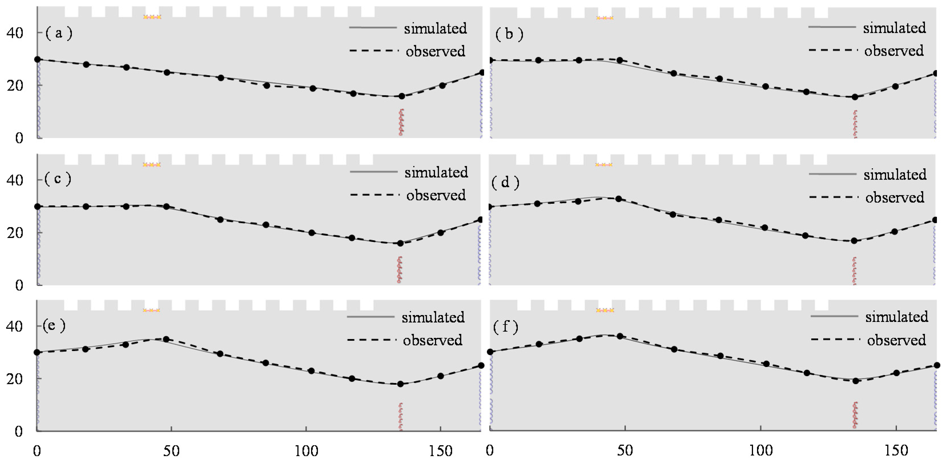
After calibration of the model, the results show good agreement between the simulated results and the measured data during the calibration period (Figure 10). Finally, the hydraulic conductivity K is 40 m/day and the specific yield is 0.1 in the numerical model. When recharge intensity is 4.8 mL/s·m at position 4, the results of the verification periods also indicated the model is stable and accuracy, so we can say that the model can represent the experimental process. 60 simulation scenarios that combined with 12 recharge sites (Figure 9) and five kinds of recharge intensity (2.4 mL/s·m, 3.6 mL/s·m, 4.8 mL/s·m, 6 mL/s·m, 7.2 mL/s·m) were adopted in the experiment. Each of them was simulated based on the developed model and compared with the measurements to get relevant groundwater levels and water balance data, respectively.
3.2. Simulation Results
3.2.1. Analysis of Water Balance
Taking the scenario with a recharge intensity of 4.8 mL/s and the recharge position 2 as an example.
The results of the water balance analysis in the part of the time period are shown in Table 3. The inflow of the aquifer mainly comes from two parts. One is lateral inflow, which comes from both sides of the Dirichlet boundary condition. The other is the amount of artificial recharge water, which comes from the Neumann boundary condition. In the initial stage of the recharge, most of the inflow water comes from the Dirichlet boundary. However, with the continuous artificial recharge process, the water inflow from the Neumann boundary gradually plays a dominant role. As for the aspect of outflow in the aquifer, it is combined with the artificial exploitation by pumping well and the lateral outflow. Lateral outflow did not occur until 30 s later at the initial stage of the recharge. Later, the lateral outflow increased constantly. This is because the height of groundwater mound is higher than the water level of the Dirichlet boundary condition, which caused part of the recharge water losses. The difference between the total amount of recharge and the total amount of discharge is the total water storage change of aquifer. It is equal to the ESC, which is concentrated in this study.
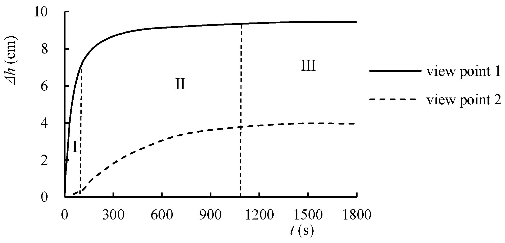
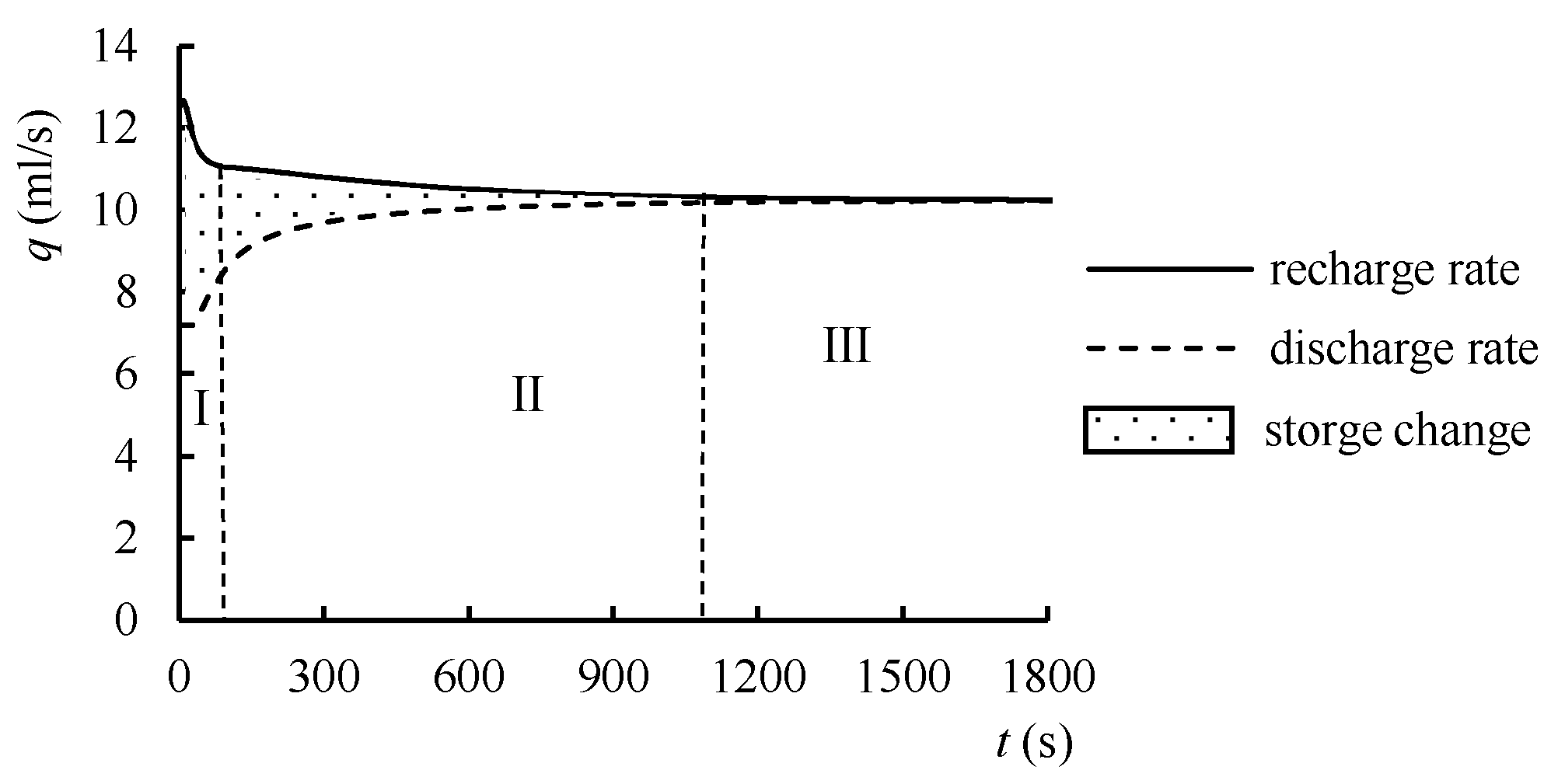
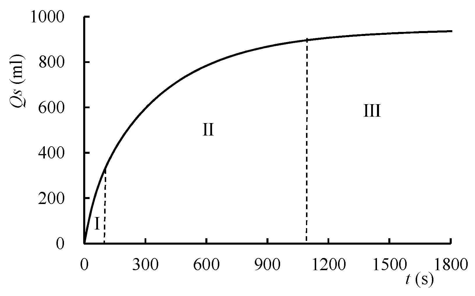
Five variables that were calculated and analyzed by the numerical simulation are the groundwater levels in observation points, the inflow and outflow rates, the ESC and the ESR of the groundwater reservoir. As shown in Figure 11, Figure 12, Figure 13 and Figure 14, the groundwater levels, inflow rate and the ESC increased with time. On the contrary, the outflow rate and the ESR decreased with time. Moreover, each variable can be divided into three similar stages during the artificial recharge process of groundwater reservoir, such as (I) response stage, (II) growth stage, and (III) stabilization stage.
The first stage is the response stage (I). In this stage, the recharge water enters into the saturated zone through the unsaturated zone, it leads to the groundwater level beginning to respond to the recharge and rise gradually. The groundwater level in observation point 1 raised much faster than the water level in observation point 2, therefore, the groundwater level under the infiltration basin is rising faster than the pumping well. It presents a significant lag effect of aquifer in the pumping well. Moreover, as shown in Figure 12, the inflow rate has decreased rapidly, while the outflow rate has increased gradually. Because the artificial recharge and exploitation are in constant flowing rates, the artificial recharge process mainly influences the water exchange rate of the lateral boundaries. The rate of discharge is stable at the beginning of this stage. 30 s later, the hydraulic gradient between the groundwater mound and the left side of lateral boundary starts to appear; it leads to some water discharge through the boundary and causes the growth of the outflow rate. Based on the law of conservation of mass, the groundwater storage variation can be simply expressed by integrating the difference between the inflow and outflow rate in Equation (5), which is equal to the area that is surrounded by the inflow rate curve and the outflow rate curve in Figure 12. Furthermore, the ESR falls down while the ESC rises rapidly. It is worth noting that the ESR increased quickly to more than 100% in the beginning, just a few seconds, and the maximum ESR can reach to 106.5%. This phenomenon is caused by the relation between recharge and discharge is changed. Then, the ESR decays fast.
where V is groundwater storage variation; qi is inflow rate; qo is outflow rate.
The second stage is the growth stage (II). The increasing rate of groundwater level is relatively stable at this stage. When compared with the first stage, the water level increases significantly slowly beneath the infiltration basin. The water level of the pumping well rises steadily and the increases almost appear in this stage. The curves of inflow rate and outflow rate are getting closer to each other, so the growth rate of groundwater variation gradually decreased. Therefore, as is shown in Figure 13 and Figure 14, the increasing rate of the ESC is reduced; it slows down the ESR decreasing rate. This change results from that some of the artificial recharge water discharge from boundaries because of the increasing of the hydraulic gradient between groundwater mound and lateral boundaries, others captured by the pumping well directly.
The final stage is the stabilization stage (III). During this period, the groundwater level becomes stable; the constant artificial recharge forms coexisting of the recharge groundwater mound and cone of depression at last. The groundwater level under infiltration basin is 36.9 cm, and the groundwater level of the pumping well is 16.2 cm. Therefore, the groundwater level raised 9.4 cm in the infiltration basin and 4.0 cm in the pumping well when compared with the initial groundwater level during the artificial recharge. It is obvious that the further from the observation point to the infiltration basin, the weaker the influence. In addition, in this stage, the inflow rate is equal to the outflow rate, and the total storage variation reach to a definite value. As for the ESC, it reaches to 946.7 mL, which is the maximum storage capacity of the underground reservoir in this scenario. The ESR decreases exponentially with the increasing of time.
3.2.2. Analysis of Influencing Factors
Based on the experiment and theoretical analysis, it can be seen that the effect of artificial recharge of underground reservoir is affected by the following factors: the position of infiltration basin, the intensity of recharge, and the period of recharge. According to Equations (1) and (2), the ESC and the ESR of all the 60 simulated scenarios were calculated by groundwater hydrologic budget. It is fitted with an anti-tangent function. By this function, the fitting goodness of each group is more than 99%, it proved that this result agrees with the simulation value approximately. As a consequence, the corresponding equations (Equations (6) and (7)) show the correlation between the ESC (Qs) and the time (t), as well as that the correlation of the ESR (β) change with time (t).
where Qmax is the maximum ESC (maximum storage capacity); a is the time parameter; and, q is the recharge intensity.
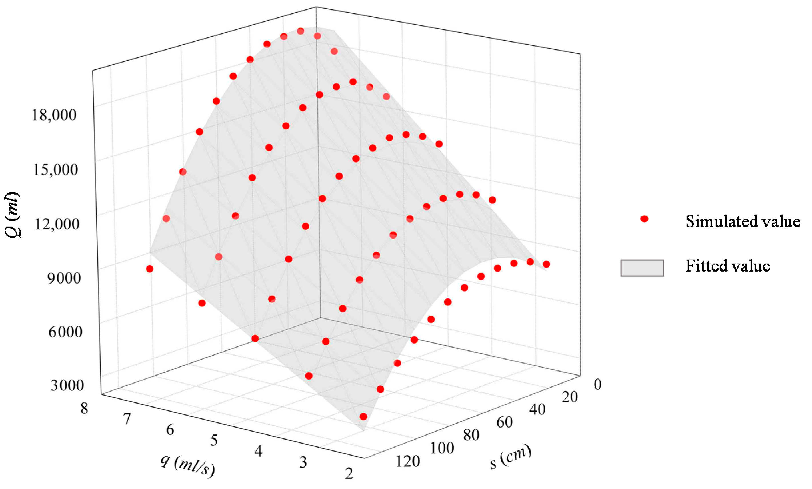
These equations suggest that the maximum ESC (Qmax) is an important index to estimate the ESC and the ESR in the study of groundwater reservoir artificial recharge effect. In this paper, Qmax is mainly affected by the recharge intensity (q) and relative distance (s) between the infiltration basin and pumping well. The correlation between Qmax and s, q (Figure 15) is shown as in the fitting equation (Equation (8)). The maximum capacity and distance would be in a quadratic function relationship. The relationship between maximum capacity and q is a linear function, which is the same as it have mentioned in the physical experiment. Using this binomial regression model can illustrate the relationship of recharge intensity and location of the infiltration basin in practical problems.
3.2.3. Analysis of the Effect of intermittent Recharge
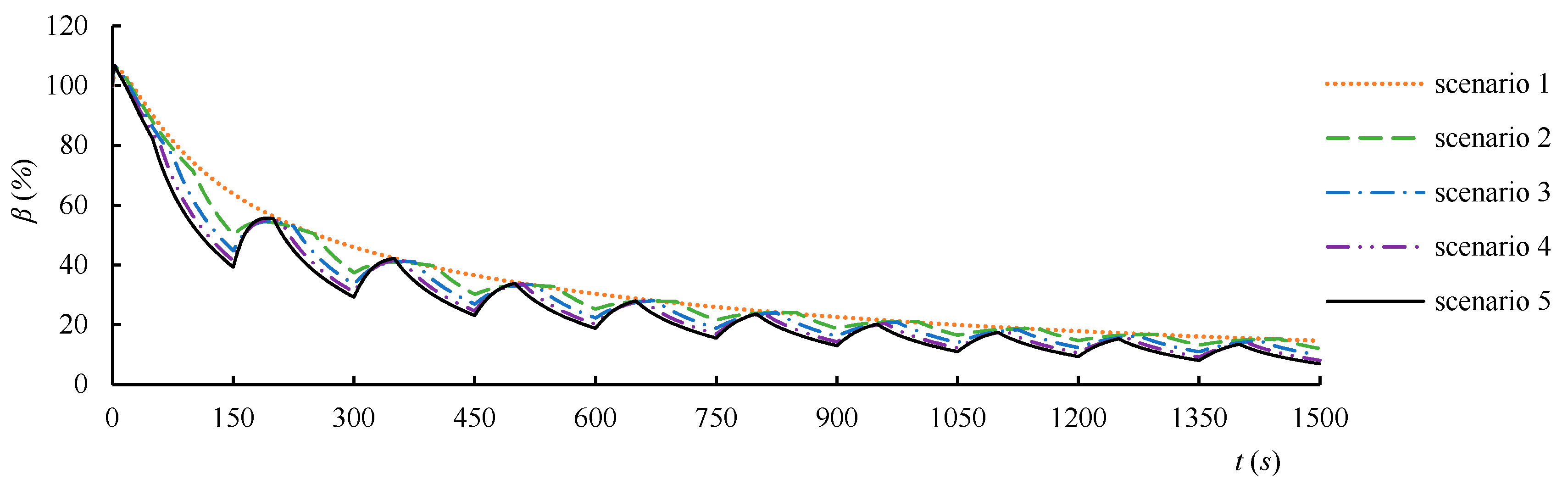
In arid regions, the source of recharge water mainly comes from summer floods, which have uneven spatiotemporal distributions. Therefore, the water shortage has high seasonality. When the water resource regulation plan of groundwater reservoir is designed, the total amount of water infiltrating into the aquifer is often limited, which requires a comprehensive consideration of recharge period, distance, and recharge intensity. For existing groundwater reservoirs that has determined infiltration basin, the recharge duration and corresponding recharge intensity were chosen to study when the recharge volume was constant. Consequently, in assuming the initial conditions, the recharge position 2 was selected to build the infiltration basin, the total water volume is 360 mL. There are ten cycles, each of them is 150 s with a total duration of 1500 s. Five scenarios were designed with different recharge intensity, recharge time, and interval time, the distribution of them were shown in Table 4. Because of the recharge water source is not directly derived from the real-time rainfall, the recharge process was generalized as a continuous and uniform process. According to the simulation results, the curves of the ESC and the ESR change with time are shown in Figure 16 and Figure 17.
From Figure 16, in first two periods starting from the periodic recharging, the short duration, and high-intensity recharge will save more water in the underground reservoir area. With the increasing time, every scenario puts up with similar change tendency. When the growth of the ESC becomes gradually stable, it is better to choose the long duration and low-intensity artificial recharge plan. The water storage changes more gently and the groundwater level fluctuation is small. However, the ESC of scenarios with short duration and high-intensity fluctuated greatly and the water quantity decreases. The change in the ESR for different recharge scenarios (Figure 17) reflects that using long duration and low-intensity recharge plan (scenario 1) is more beneficial to the storage of water. Therefore, the recharge period should be taken into consideration in the water resources regulation plan optimization; one can even think about changing the regulation plan at a different stage of the artificial recharge.
4. Conclusions
With the results from physical experiments and numerical simulations, this paper has demonstrated that the effect of artificial recharge on groundwater reservoir is controlled by infiltration basin. The ESC and ESR can help to reflect the effect of artificial recharge, when all of the hydrogeological parameters were the same in all of the simulations. They are influenced by infiltration basin position, recharge intensity, and recharge period.
Experiment results demonstrated that the location of the infiltration basin is actually controlled by the hydrogeological conditions. The infiltration basin should be sited further away from the hydraulic boundary to release the discharge from the boundary condition. It is beneficial to store more water in the aquifer by properly shortening the distance between the infiltration basin and the pumping well, but the distance should not be too close. The range of distance from 10 cm to 70 cm can be accepted as the alternative positions. Taking into account the transport distance from the recharge source, position 6, which is 70 cm far away from pumping well, is the best choice to build an infiltration basin. The increasing of recharge intensity can lead to the growth of storage capacity and the reduction of artificial recharge efficiency.
The simulation results of groundwater reservoir showed that there is close relationship between groundwater levels, inflow and outflow rates, and the ESC and the ESR during the artificial recharge process. Moreover, this process can be divided into three stages: response stage, growth stage, and stable stage. Through the analysis of the simulation results, the time-varying characteristics of the ESC and the ESR are controlled by the maximum storage capacity. Furthermore, the relationship between the maximum capacity and the relative distance from the pumping well to the infiltration basin is in accordance with a quadratic function, and the relationship between maximum capacity and recharge intensity is a linear function.
Based on the numerical model, different scenarios, which have same total water volume, were designed to simulate intermittent recharge. Simulation results show that the intermittent recharge is affected by various factors, such as recharge intensity, recharge duration, regulation aim, and regulation period. In first two periods, the short duration and high-intensity recharge will save more water. With the increasing time, the long duration and low-intensity scenario gained superiority. Using long duration and low-intensity recharge plan get high ESR. It should be considered according to the practical conditions and choose a reasonable water resource regulation plan.
Acknowledgments
The research work was funded by the National Natural Science Foundation of China project entitled “Study on Water Cycle Evolution of Groundwater Reservoir in the Arid Area under Artificial Regulation” (No. 41572210).
Author Contributions
All the authors participated in every step of this research. In particular, Yang Xu did the physical experiment conditions and analyzed the method for the experimental result. Longcang Shu established the FEFLOW model and finished the calibration and verification work. Longcang Shu also supervised the entire research project. Yongjie Zhang analyzed numerical simulation result. Peipeng Wu designed and analyzed the regulation plan of groundwater reservoir. Abunu Atlabachew Eshete and Esther Chifuniro Mabedi joined the experiment and polished up this article.
Conflicts of Interest
The authors declare no conflict of interest.
References
- Scanlon, B.R.; Keese, K.E.; Flint, A.L.; Flint, L.E.; Gaye, C.B.; Edmunds, W.M.; Simmers, I. Global synthesis of groundwater recharge in semiarid and arid regions. Hydrol. Process. 2006, 20, 3335–3370. [Google Scholar] [CrossRef]
- Orellana, F.; Verma, P.; Ii, S.P.L.; Daly, E. Monitoring and modeling water-vegetation interactions in groundwater-dependent ecosystems. Rev Geophys. 2012, 50, RG3003. [Google Scholar] [CrossRef]
- Zhao, T.S. Discussion of problems for groundwater reservoir. Hydrogeol. Eng. Geol. 2002, 29, 65–67. (In Chinese) [Google Scholar]
- Li, L.W.; Shu, L.C.; Yin, Z.Z. Concept and design theory of groundwater reservoir. J. Hydraul. Eng. 2006, 13, 123–132. [Google Scholar]
- Pyne, R.D.G. Groundwater Recharge and Wells: A Guide to Aquifer Storage and Recovery; CRC Press: Boca Raton, FL, USA, 1995; p. 401. [Google Scholar]
- Ward, J.D.; Simmons, C.T.; Dillon, P.J. A theoretical analysis of mixed convection in aquifer storage and recovery: How important are density effects? J. Hydrol. 2007, 343, 169–186. [Google Scholar] [CrossRef]
- Page, D.W.; Peeters, L.; Vanderzalm, J.; Barry, K.; Gonzalez, D. Effect of aquifer storage and recovery (ASR) on recovered stormwater quality variability. Water Res. 2017, 117, 1–8. [Google Scholar] [CrossRef] [PubMed]
- Zhang, G.; Feng, G.; Li, X.; Xie, C.; Pi, X. Flood effect on groundwater recharge on a typical silt loam soil. Water 2017, 9, 523. [Google Scholar] [CrossRef]
- Ong’Or, B.T.I.; Shu, L.C. Groundwater overdraft and the impact of artificial recharge on groundwater quality in a cone of depression, Jining, China. Water Int. 2009, 34, 468–483. [Google Scholar] [CrossRef]
- Zhang, Y.; Wu, J.C.; Xue, Y.Q.; Wang, Z.C.; Yao, Y.G.; Yan, X.X.; Wang, H.M. Land subsidence and uplift due to long-term groundwater extraction and artificial recharge in Shanghai, China. Hydrogeol. J. 2015, 23, 1851–1866. [Google Scholar] [CrossRef]
- Shi, X.Q.; Jiang, S.M.; Xu, H.X.; Jiang, F.; He, Z.F.; Wu, J.C. The effects of artificial recharge of groundwater on controlling land subsidence and its influence on groundwater quality and aquifer energy storage in Shanghai, China. Environ. Earth 2016, 75, 1–18. [Google Scholar] [CrossRef]
- Sophiya, M.S.; Syed, T.H. Assessment of vulnerability to seawater intrusion and potential remediation measures for coastal aquifers: A case study from eastern India. Environ. Earth. 2013, 70, 1197–1209. [Google Scholar] [CrossRef]
- Thompson, A.; Nimmer, M.; Misra, D. Effects of variations in hydrogeological parameters on water-table mounding in sandy loam and loamy sand soils beneath stormwater infiltration basins. Hydrogeol. J. 2010, 18, 501–508. [Google Scholar] [CrossRef]
- Nimmer, M.; Thompson, A.; Misra, D. Modeling water table mounding and contaminant transport beneath stormwater infiltration basins. J. Hydrol. Eng. 2010, 15, 963–973. [Google Scholar] [CrossRef]
- Du, S.H.; Su, X.X.; Zhang, W.J. Effective storage rates analysis of groundwater reservoir with surplus local and transferred water used in Shijiazhuang City, China. Water Resour. Manag. 2013, 27, 157–169. [Google Scholar] [CrossRef]
- Dillon, P. Future management of aquifer recharge. Hydrogeol. J. 2005, 13, 313–316. [Google Scholar] [CrossRef]
- Maréchal, J.C.; Dewandel, B.; Ahmed, S.; Galeazzi, L.; Zaidi, F.K. Combined estimation of specific yield and natural recharge in a semi-arid groundwater basin with irrigated agriculture. J. Hydrol. 2006, 329, 281–293. [Google Scholar] [CrossRef]
- Stauffer, F.; Attinger, S.; Zimmermann, S.; Kinzelbach, W. Uncertainty estimation of well catchments in heterogeneous aquifers. Water Res. 2002, 38, 20–21. [Google Scholar] [CrossRef]
- Manghi, F.; Mortazavi, B.; Crother, C.; Hamdi, M.R. Estimating regional groundwater recharge using a hydrological budget method. Water Resour. Manag. 2009, 23, 2475–2489. [Google Scholar] [CrossRef]
- Hernández-Espriú, A.; Arango-Galván, C.; Reyes-Pimentel, A.; Martínez-Santos, P.; Paz, C.P.D.L.; Macías-Medrano, S. Water supply source evaluation in unmanaged aquifer recharge zones: The mezquital valley (Mexico) case study. Water 2016, 9, 4. [Google Scholar] [CrossRef]
- Sharda, V.N.; Kurothe, R.S.; Sena, D.R.; Pande, V.C.; Tiwari, S.P. Estimation of groundwater recharge from water storage structures in a semi-arid climate of India. J. Hydrol. 2006, 329, 224–243. [Google Scholar] [CrossRef]
- Crosbie, R.S.; Binning, P.; Kalma, J.D. A time series approach to inferring groundwater recharge using the water table fluctuation method. Water Resour. Res. 2005, 41, 287–295. [Google Scholar] [CrossRef]
- Niazi, A.; Prasher, S.O.; Adamowski, J.; Gleeson, T. A system dynamics model to conserve arid region water resources through aquifer storage and recovery in conjunction with a dam. Water 2014, 6, 2300–2321. [Google Scholar] [CrossRef]
- Kasper, J.W.; Denver, J.M.; McKenna, T.E.; Ullman, W.J. Simulated impacts of artificial groundwater recharge and discharge on the source area and source volume of an Atlantic coastal plain stream, Delaware, USA. Hydrogeol. J. 2010, 18, 1855–1866. [Google Scholar] [CrossRef]
- Edwards, E.C.; Harter, T.; Fogg, G.E.; Washburn, B.; Hamad, H. Assessing the effectiveness of drywells as tools for stormwater management and aquifer recharge and their groundwater contamination potential. J. Hydrol. 2016, 539, 539–553. [Google Scholar] [CrossRef]
- Clement, T.P.; Kim, Y.C.; Gautam, T.R.; Lee, K.K. Experimental and numerical investigation of DNAPLdissolution processes in a laboratory aquifer model. Groundwater Monit. Remediat. 2004, 24, 88–96. [Google Scholar] [CrossRef]
- Hans, J.G. DHI-WASY Software FEFLOW Reference Manual; DHI WASY GmbH: Berlin, Germany, 2005. [Google Scholar]
- Nash, J.E.; Sutcliffe, J.V. River flow forecasting through conceptual models part I—A discussion of principles. J. Hydrol. 1970, 10, 282–290. [Google Scholar] [CrossRef]
Figure 1.
Diagram of physical experiment device.

Figure 2.
Result of grain size analysis.
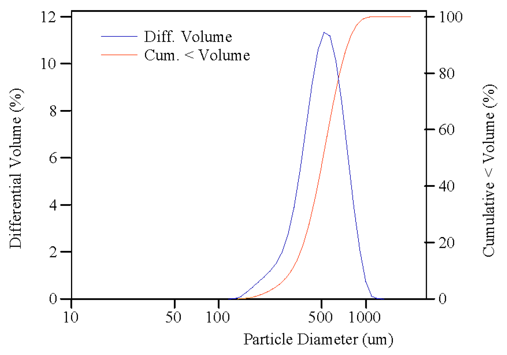
Figure 3.
Water storage area calculation method.
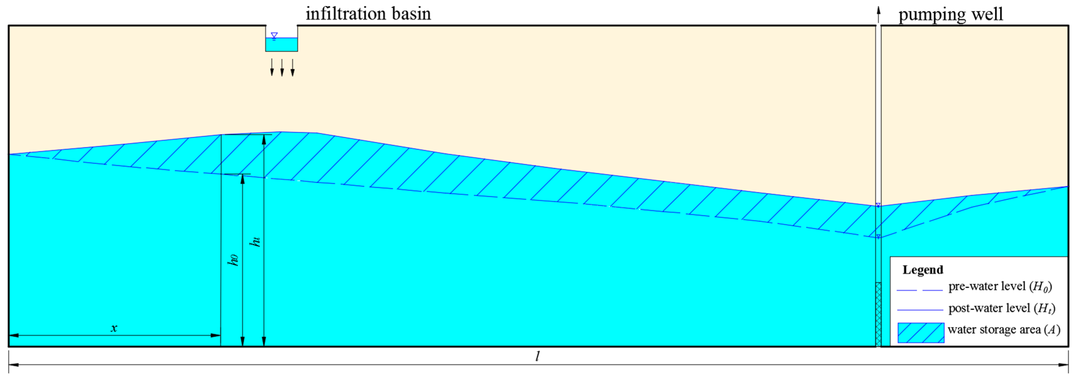
Figure 4.
The effective storage capacity (ESC) (Qs)—distance (s) relationship curves.

Figure 5.
The effective storage rates (ESR) (β)—distance (s) relationship curves.

Figure 6.
The ESC (Qs)—recharge intensity (q) relationship curves.

Figure 7.
The ESR (β)—recharge intensity (q) relationship curves.

Figure 8.
Initial conditions of simulation model.
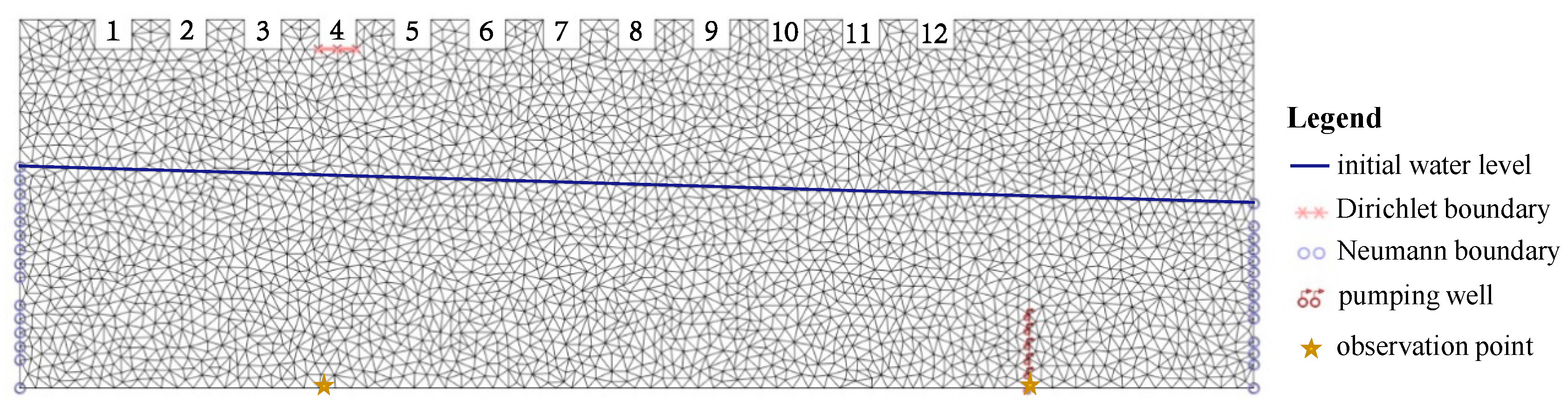
Figure 9.
Comparison between observed and simulated groundwater levels at pressure sensor point 2, 5, 8.
Figure 9.
Comparison between observed and simulated groundwater levels at pressure sensor point 2, 5, 8.
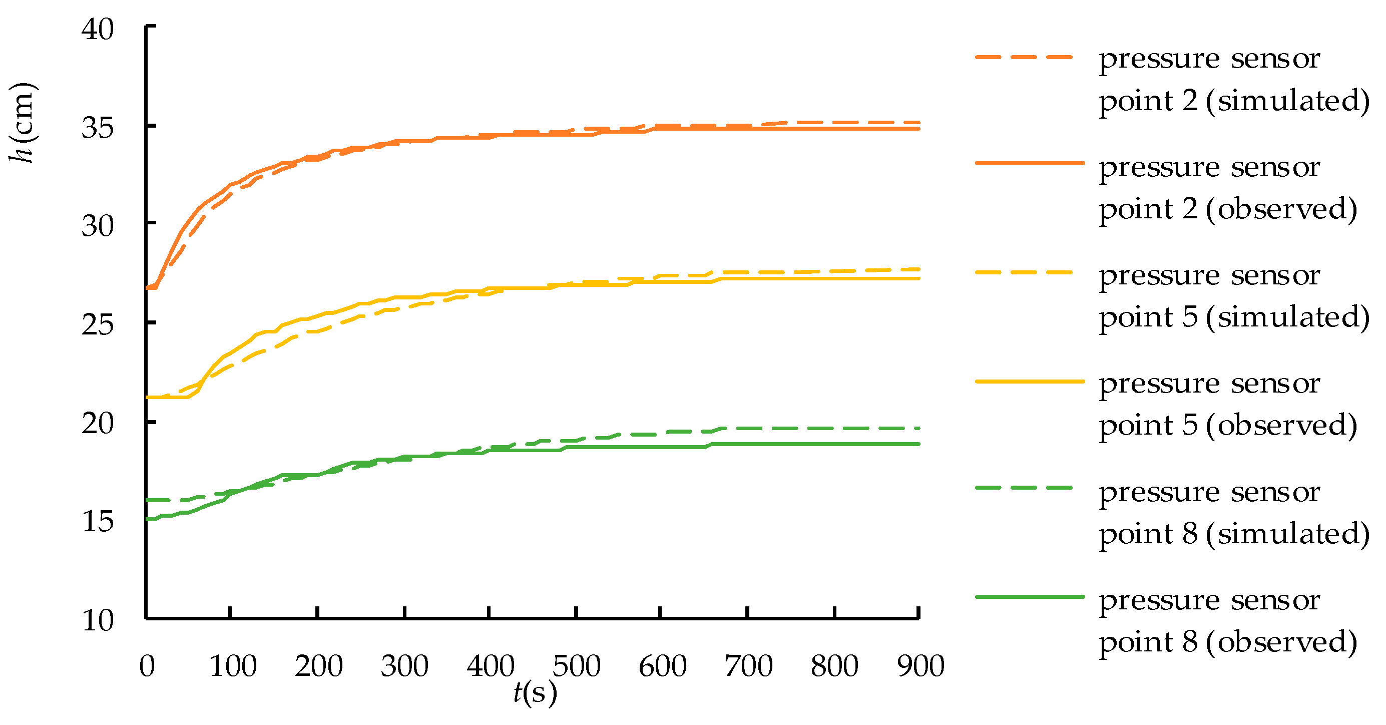
Figure 10.
Comparison between observed and simulated groundwater levels at time of: (a) 0 min; (b) 1 min; (c) 2 min; (d) 3 min; (e) 5 min; and, (f) 15 min.
Figure 10.
Comparison between observed and simulated groundwater levels at time of: (a) 0 min; (b) 1 min; (c) 2 min; (d) 3 min; (e) 5 min; and, (f) 15 min.

Figure 11.
Groundwater level change in observation points.

Figure 12.
Calculation method of groundwater storage variation.

Figure 13.
The ESC (Qs)—time (t) relationship curves.

Figure 14.
The ESR (β)—time (t) relationship curves.
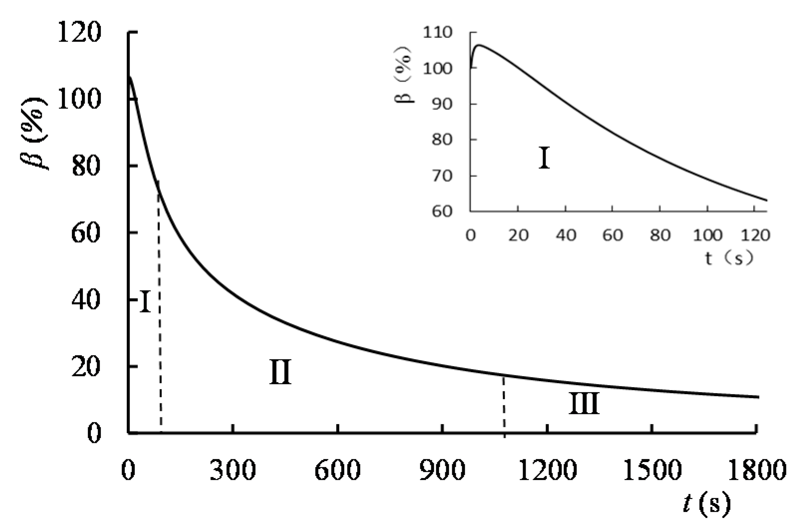
Figure 15.
Qmax binomial regression model.

Figure 16.
Curves of ESC (Q) change with time for different scenarios.
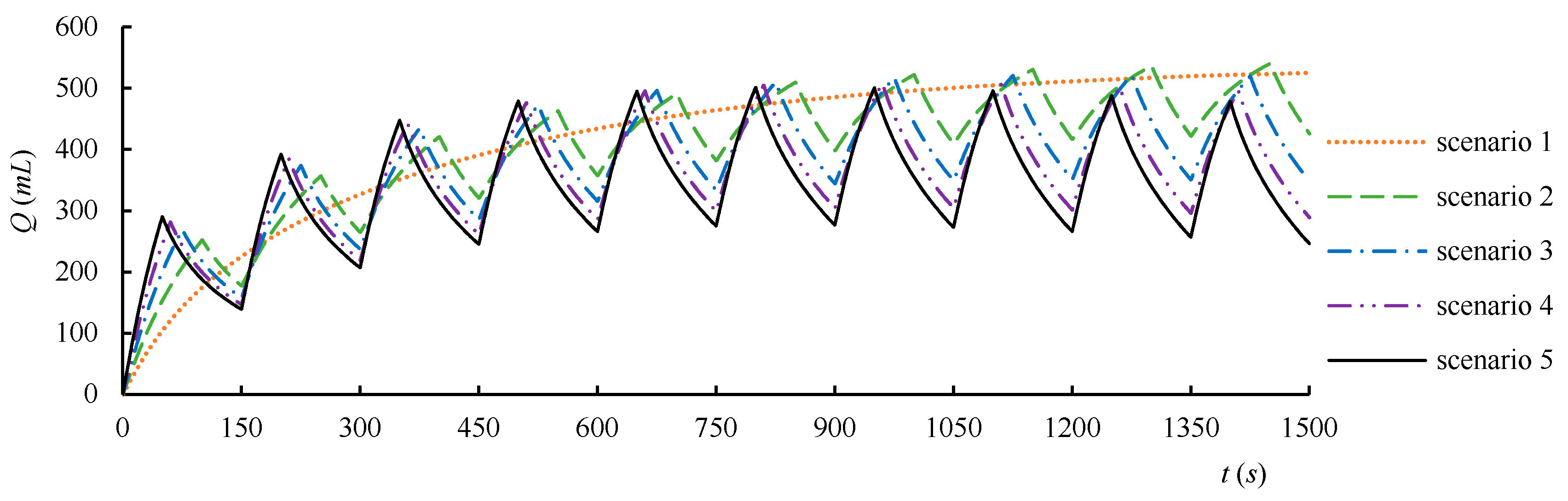
Figure 17.
Curves of ESR (β) change with time for different scenarios.


Table 1.
Result of particle size analysis.
| Content (%) | <10 | <25 | <50 | <75 | <90 | Average | Mid-Value |
|---|---|---|---|---|---|---|---|
| Diameter(um) | 310.5 | 401.8 | 509.6 | 630.8 | 749.8 | 520.4 | 509.6 |
Table 2.
Nash-Sutcliffe efficiency (NSE) in pressure sensor points.
| Pressure Sensor Point | 2 | 5 | 8 |
|---|---|---|---|
| NSE | 0.973 | 0.936 | 0.797 |
Table 3.
Results of water budget.
| Time Period (s) | Inflow | Outflow | Storage Variation (mL) | ||||||||
|---|---|---|---|---|---|---|---|---|---|---|---|
| Lateral Inflow | Artificial Recharge | Total (mL) | Lateral Outflow | Artificial Exploitation | Total (mL) | ||||||
| Quantity (mL) | Percentage (%) | Quantity (mL) | Percentage (%) | Quantity (mL) | Percentage (%) | Quantity (mL) | Percentage (%) | ||||
| 0.0 | 0.0 | - | 0.0 | - | 0.0 | 0.0 | - | 0.0 | - | 0.0 | 0.0 |
| 1.3 | 80.7 | 57.0 | 60.8 | 43.0 | 141.5 | 0.0 | 0.0 | 81.0 | 100.0 | 81.0 | 60.5 |
| 14.0 | 825.1 | 56.4 | 638.7 | 43.6 | 1463.8 | 0.0 | 0.0 | 837.5 | 100.0 | 837.5 | 626.3 |
| 32.3 | 1800.3 | 54.6 | 1495.4 | 45.4 | 3295.8 | 1.1 | 0.1 | 1936.4 | 99.9 | 1937.6 | 1358.2 |
| 79.3 | 3944.7 | 51.5 | 3717.6 | 48.5 | 7662.3 | 234.7 | 4.7 | 4758.5 | 95.3 | 4993.2 | 2669.1 |
| 145.6 | 6810.0 | 49.8 | 6874.0 | 50.2 | 13,684.0 | 1094.1 | 11.1 | 8735.2 | 88.9 | 9829.3 | 3854.7 |
| 325.5 | 14,323.1 | 48.1 | 15,475.6 | 51.9 | 29,798.7 | 4519.6 | 18.8 | 19,529.9 | 81.2 | 24,049.5 | 5749.2 |
| 581.7 | 24,470.1 | 46.9 | 27,748.2 | 53.1 | 52,218.3 | 10,231.7 | 22.7 | 34,902.2 | 77.3 | 45,133.8 | 7084.4 |
| 1244.3 | 49,380.7 | 45.3 | 59,517.9 | 54.7 | 108,898.6 | 26,141.8 | 25.9 | 74,659.8 | 74.1 | 100,801.7 | 8096.9 |
| 1800.0 | 69,855.7 | 44.8 | 86,175.5 | 55.2 | 156,031.2 | 39,776.7 | 26.9 | 108,000.0 | 73.1 | 147,776.7 | 8254.5 |
Table 4.
Scenarios of different recharge period.
| Scenario | Scenario 1 | Scenario 2 | Scenario 3 | Scenario 4 | Scenario 5 |
|---|---|---|---|---|---|
| recharge intensity (mL/s) | 2.4 | 3.6 | 4.8 | 6 | 7.2 |
| recharge time(s) | 150 | 100 | 75 | 60 | 50 |
| interval time(s) | 0 | 50 | 75 | 90 | 100 |
© 2017 by the authors. Licensee MDPI, Basel, Switzerland. This article is an open access article distributed under the terms and conditions of the Creative Commons Attribution (CC BY) license (http://creativecommons.org/licenses/by/4.0/).
Share and Cite
MDPI and ACS Style
Xu, Y.; Shu, L.; Zhang, Y.; Wu, P.; Atlabachew Eshete, A.; Mabedi, E.C. Physical Experiment and Numerical Simulation of the Artificial Recharge Effect on Groundwater Reservoir. Water 2017, 9, 908. https://doi.org/10.3390/w9120908
AMA Style
Xu Y, Shu L, Zhang Y, Wu P, Atlabachew Eshete A, Mabedi EC. Physical Experiment and Numerical Simulation of the Artificial Recharge Effect on Groundwater Reservoir. Water. 2017; 9(12):908. https://doi.org/10.3390/w9120908
Chicago/Turabian StyleXu, Yang, Longcang Shu, Yongjie Zhang, Peipeng Wu, Abunu Atlabachew Eshete, and Esther Chifuniro Mabedi. 2017. "Physical Experiment and Numerical Simulation of the Artificial Recharge Effect on Groundwater Reservoir" Water 9, no. 12: 908. https://doi.org/10.3390/w9120908
Note that from the first issue of 2016, this journal uses article numbers instead of page numbers. See further details here.