1. Introduction
How can one predict the complex time-dependence of the cumulative infiltration into a soil? Why do estimates of evapotranspiration (ET) at different spatial scales differ? What do infiltration and ET have in common and how do they differ? An initial attempt to answer these questions within the context of percolation theory is given here.
When rain falls upon an unsaturated porous medium such as dry soil, some runs off, some evaporates from the terrestrial surface, and some infiltrates into the medium. Of the latter, a fraction is taken up by the plants through the roots and evaporated from the stomata (a process termed transpiration), and the remainder continues downward to the water table (net infiltration or deep percolation). While the total return of water to the atmosphere includes evaporation and transpiration, known as evapotranspiration (quantities often measured together), our focus is on the plant pathway. Both transpiration and infiltration are instrumental in the drawdown of CO2 from the atmosphere, the former through photosynthesis, the latter through chemical weathering. In each case, water is critical for the chemistry: in transpiration, for transporting the CO2 from the atmosphere, plant roots and decaying organic material; in infiltration, as a reagent and as an agent to bring nutrients to plant roots, and thus facilitate nutrient uptake.
The fact that water carries reactive solutes or nutrients with it is relevant to the processes of weathering and vegetation growth, among others. The mathematical treatment of reactive solute transport is a possible source of techniques to address unsteady flow, since the majority of solute transport appears to be non-Gaussian1 [
1]. Such non-Gaussian transport is generally inconsistent with the Gaussian transport predicted by the Advection–Dispersion Equation (ADE), a formulation which is echoed in the treatment of unsteady flow using the Richards’ equation [
2]. Thus, particularly if infiltration experiments do not prove consistent with the Richards’ equation, there may be a motivation to address such discrepancies within the framework of non-Gaussian transport theories. While a wide range of mathematical techniques have been applied to generate non-Gaussian transport, including the Continuous Time Random Walk, or CTRW (see recent review in [
3]), to our knowledge, the only technique that has also been adapted to the problem of variable infiltration is the fractional derivative, familiar from Fractional Advection Dispersion Equation (FADE) applications [
4]; see [
5] for application of the FADE to infiltration.
Scaling laws for solute transport based on percolation concepts, originally proposed by [
6] and followed up by [
7,
8], have recently been applied to the growth and development of plants [
9,
10], as well as for chemical weathering (see e.g., [
11,
12]). These scaling laws treat the advective spreading of solutes into a medium that is originally fully filled with pure water, or is in the process of saturation. It is the effective “compressibility” of solutes (changing the volume of a plume as it spreads) that distinguishes solute transport from water flow under steady flow conditions, and leads to the significant non-Gaussian characteristics of the transport [
11]. In unsaturated, unsteady flow, water spreads (imbibes) into a medium that is originally filled with air, in contrast to steady flow, for which the medium water content does not change. In both cases, the mass advected into the medium is presumed to preferentially follow paths of optimal flow as described in percolation theory, making a predictive approach based on analogy attractive. Importantly, both unsteady flow and solute transport are treated traditionally (in continuum mechanics) as diffusive processes [
13]; however, advection of solutes into such a medium is distinctively different from diffusion [
12]. The analogy between water infiltration and solute transport in terms of the concept of compressibility thus suggests that the same scaling framework that works for chemical weathering and plant growth can be applied towards unsteady water infiltration.
Therefore, the main objectives of this study are (1) to develop theoretical scaling laws for infiltration and transpiration processes in soils under unsteady flow conditions (e.g., the optimal transport distances and the most likely transport time, respectively); and (2) to compare the proposed models with experimental data. Below, we review the scaling theory of solute transport, followed by a brief discussion of scaling arguments linking vegetation growth [
9] and soil formation [
14].
2. Theory
In the following, we overview the classical theory of unsteady flow or solute transport only, as their results can be contrasted with the predictions of percolation theory. Since percolation theory (see e.g., [
15,
16]) is critical to the hypotheses tested in this manuscript, we turn to that subject first. Percolation theory comes in the three variants: site, bond and continuum (corresponding to volume fraction). Following [
17,
18], Hunt [
19] has advocated using percolation formulas adapted to continuum percolation problems for predicting flow and transport phenomena of porous media. The reason is that, with the wide range of pore sizes and local coordination numbers, it is difficult to place such media on any kind of regular grid. Nevertheless, Sahimi [
20] showed that wetting, in which water must occupy an entire pore, is a site percolation problem in principle, while drying, for which water must exit through a pore neck, should be conceptualized as a bond percolation problem. Either is more properly treated as an invasion percolation problem than as a random percolation problem while the fluid, either air or water, is incompressible at the pore scale. Such pore-scale incompressibility allows fluid to become trapped in pores rather than displaced, when a second fluid invades. Thus, wetting is invasion site percolation with trapping, drying is invasion bond percolation with trapping, and fully saturated conditions are termed random percolation. This classification scheme is important if one seeks relevant information on various percolation scaling predictions, as we do below.
One useful application from percolation theory is critical path analysis (CPA) developed to find dominant paths of charge or fluid flow through heterogeneous media [
19,
21,
22]. The concept is most easily understood in a network model constructed of pore bodies connected through pore throats (see e.g., [
23]), for which the difficulty of flow is localized along the connections between pores and discretized accordingly. Within the percolation theory framework, sites and bonds are equivalent to bodies and throats in a network of pores, respectively. The strategy of CPA is to apply the percolation threshold—the minimum fraction required to form the sample-spanning cluster and let the system percolate—to the spread of local resistance values in order to find the most resistive element on the most highly conductive (or permeable) interconnected path through the system. Sahimi [
16] observed that solute transport along such optimal paths as described in percolation theory should follow the same scaling laws as solute transport through actual percolation clusters. Here, we extend that conjecture to unsteady flow as well.
Percolation Scaling Theory for Solute Transport
Percolation theory provides a promising framework that has been widely applied to study flow and transport in interconnected networks and media. Percolation theory combines microscopic characteristics of a medium with its topological properties to determine macroscopic quantities, such as conductivity, permeability, and dispersion. A full theoretical treatment of the scaling of solute transport is beyond the scope of the present work, as we are interested in distances and times such as minimum and optimal transport distances and the most likely transport time as a function of system size, rather than arrival time distributions. The most likely transport time has been found to generate transport velocities and fluxes reasonably accurately for up to five orders of magnitude of time [
12]. For a comprehensive review of percolation theory applications on fluid flow and solute transport, see [
16,
24,
25].
Percolation theory applies most simply to porous media for which flow or conduction along bonds (pore throats) between nodes (pore bodies) is either possible or impossible [
26]. Here, it delivers relatively simple scaling laws for, e.g., conduction or flow properties. Such binary media can be represented by networks with resistances of value 1 or infinity, but are not characteristic of typical natural porous media, since flow is strongly pore-size dependent and pore size typically spans several orders of magnitude. Instead of bond percolation, continuum percolation has been used [
17,
18,
19] to address flow in more realistic pore networks, with irregular lattices made of pores of different sizes and shapes. In media with a wide range of pore sizes, critical path analysis [
21,
22] utilizes the percolation threshold value to generate a percolating sub-network composed of all resistances less than or equal to a “critical” value, a technique which can provide effective flow parameters such as conductivity or permeability [
19]. Thus, a sub-network composed of all the resistances less than or equal to a “critical” value just percolates. The importance in the present context is that Sahimi argued already more than 20 years ago [
16] that solute transport in real porous media with wide ranges of pore sizes should also follow percolation scaling results because of the concentration of the flow along such critical paths. Because critical path analysis is applicable to virtually all natural soils [
27], percolation theory is equally relevant to solute transport; thus, we begin by listing solute transport results from percolation theory.
Lee et al. [
6] addressed the spatiotemporal scaling of solutes transported across a two-dimensional system at the percolation threshold. The authors found that for a line source of solute in a system of length
x, the minimum path length,
L, for particles exiting on the opposite face scales with
x as
, with a most likely time of
, where
Dmin and
Db are the chemical paths exponent and the fractal dimensionality of the percolation backbone, respectively. However, when the medium is
highly heterogeneous, e.g., with a wide range of pore sizes, the length
L of the optimal paths that provide the most rapid transport across the system is proportional to the system length to a different exponent,
Dopt, rather than to
Dmin [
28,
29].
Dopt is the so-called optimal paths exponent, and is determined for the heterogeneous limit [
30]. The values of the exponents determined by [
30] are mostly accurate to five significant figures, but the optimal paths exponent only to three. The most important distinctions in porous media that affect the exponents
Db and
Dmin relate to the connectivity of the paths and the specific percolation conditions: (i) imbibition (wetting) conditions correspond to site invasion percolation with trapping; (ii) drying conditions to invasion percolation with trapping; and (iii) saturated flow to random percolation [
20]. Following [
6] the minimum path length
L is (using
Dmin from [
30]):
where
x0 is the bond length, and 2D and 3D refer to two and three dimensional systems. In the case of porous media,
x0 corresponds to the inter-pore distance or a typical grain size. Numerical prefactors of order unity are less well constrained, hence omitted from Equations (1) and (2). The value of the exponent
Dopt in 2D (for all conditions of saturation), 1.21, is similar to the value of
Dmin for 2D imbibition or drainage, 1.21, and the optimal path lengths
L scale the same as the shortest paths for imbibition or drainage,
L =
x0(
x/
x0)
1.21. In 3D
Dopt = 1.46. Similarly, the most likely travel time
is [
30]
We note that the exponent for 3D imbibition, 1.861, differs from the value for saturated conditions, 1.87 (Equation (3)). As we discuss in
Section 6, such a small discrepancy actually leads to detectable differences in scaling of the cumulative infiltration. Although the conditions we address are (1) for vertical infiltration, wetting, 3D flow; and (2) for transpiration, desaturating 2D flow, we include the entire suite of values of these exponents in case conditions addressed in other investigations are different. In particular, swelling soils may develop mudcracks on drying, providing preferential flow topologies for imbibition that are constrained to two-dimensional surfaces.
In Equations (1)–(4),
t0 is the time for fluid to traverse a distance
x0, such that
v0 =
x0/
t0 is the fluid flow rate at the pore scale. The contrast between the exponent 1.87 for the most likely time and 1.37 for the shortest distance (for 3D saturated conditions) helps explain why paths that do not appear to be extraordinarily tortuous (20 m in a 1 m column) can still retard the arrival of solutes by an enormous factor [
11] (over 1000). Since we are interested in (1) vegetation growth and transpiration in 2D (optimal paths exponent); and (2) unsteady flow in 3D (for the wetting conditions in Philip’s infiltration theory), we select here the following exponent values (from Equations (1)–(4)): (i)
Dopt (2D) =1.21 for vegetation growth, and (ii)
Db (3D imbibition) = 1.861 for vertical infiltration. These two exponents are essentially the same as the two values assumed relevant [
9,
12] for soil formation (1.87) and vegetation growth (1.21), although as a result, our analogy to soil formation and chemical weathering is not quite precise. In [
12], for example, soil was assumed to form under either saturated or saturating conditions, but only the exponent 1.87 was used. Given all the uncertainties in soil formation processes operating at time scales of up to tens of millions of years, ignoring the possibility that the appropriate exponent might, for some fraction of the time, be 1.861, seemed justified. However, in unsteady infiltration experiments, of much shorter duration and with much greater control, the exponent is constrained conceptually to be 1.861.
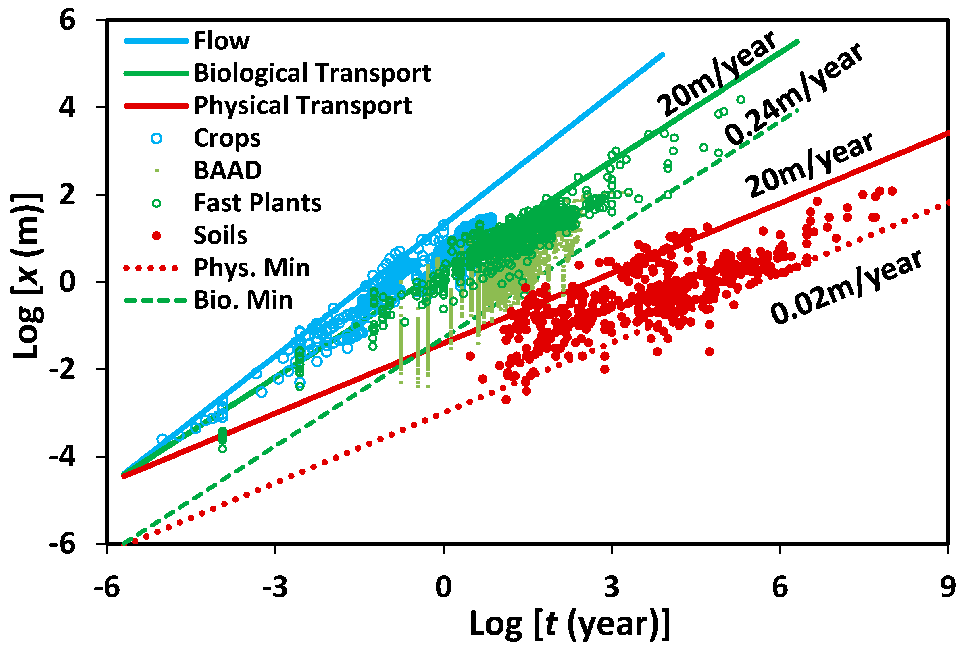
4. Relevance of Percolation Scaling to Vegetation Growth and Soil Formation
The primary purposes in this section are: (1) to show the basis of the pore-scale link between vegetation growth and soil formation; (2) provide a basis for upscaling the pore-scale water flow rate controlling vegetation growth to growing season transpiration rates, as addressed in the next section. This provides both a context and a method for the following topics.
Hunt [
9,
14] showed that the relationship
with
Db = 1.87 (for 3D flow connectivity) and
x0 a typical grain diameter predicts soil depths over an extensive range of time scales (a decade to 100 Ma), where
v0 =
x0/
t0 was taken to be the pore-scale infiltration rate. Equation (5) provides a soil formation rate of
Rs =
dx/
dt = 0.53
v0(
x/
x0)
−0.87 or 0.53
v0 (
t/
t0)
−0.46. Furthermore, ref. [
12] showed that the related scaling of solute transport rates (from the velocity of the centroid of the solute spatial distribution) could predict soil formation rates at time scales of up to 60 Ma, and that that the predicted proportionality of
Rs to
v0 is in accordance with the observed four orders of magnitude variability in
Rs when precipitation also varied over four orders of magnitude (from the Atacama desert to the New Zealand Alps). Thus, rate of flow of water through the surface medium is responsible for much of the variability in soil formation rates.
Considering vegetation linear extent (root radial extent, RRE, or plant height), Hunt and Manzoni [
9,
10] showed that
with
Dopt = 1.21 (2D) and
x0 taken as a typical pore diameter (~10, the geometric mean plant xylem diameter, Watt [
33] hold for time scales ranging from minutes to 100 kyr. In this case,
x is either the plant height, or the root radial extent, which have been shown to be closely equivalent over time scales from a growing season to about 40 years [
10,
34,
35,
36,
37]. Once again,
v0 =
x0/
t0 is the pore-scale flow rate, ranging here from about 24 cm/year to 20 m/year. This is a similar, though narrower range of flow rates than those relevant for soils under typical conditions i.e., about 2.0 cm/year to 20 m/year. The soil depths and the linear extent of natural vegetation computed from Equations (5) and (6) are given in
Figure 1. The vegetation data incorporate a wide range of data sets: at time scales from minutes to days, these are root tip extension rates, for weeks to hundreds of years, they are plant heights (which are a proxy for root radial extent over most of this range), and for thousands of years up, the measurements are subsurface extents of clonal organisms, such as
Posidonia oceanica and various tree species, or fungi. We note that the leaf area index could also be used to characterize plant growth [
38], instead of plant height. At the longest time scales, the soil data are mostly paleosols and laterites. At the shortest time scales, the soil data include primarily soil formation after disturbances, such as landslides, glacial retreat, or tree-throw. For typical pore and particle size of 10 μm and 30 μm, respectively, the presented pore scale velocities bound the data. We point out that since larger pores have a smaller retention capacity as they are easily drained, their contribution to plant growth is smaller [
33]. We will apply essentially the same Equations (5) and (6) to vertical infiltration and horizontal flow associated with transpiration, respectively.
5. Potential Relationship with Unsteady Flow
At spatial and temporal scales larger than the (pore) scales considered above, we hypothesize that the ratio of a transpiration depth to a transpiration time scale can take the place of the pore-scale flow velocity
v0 =
x0/
t0. Thus,
x0/
t0 →
xg/
tg, where
xg is the transpiration during a growing season (measured typically as a depth) and
tg is the length of the growing season. Using this hypothesis, we rewrite the scaling for vegetation growth in Equation (6) as
Furthermore, using total ET depths
xg (instead of transpiration data, which is much less abundant) that range from 0.02 m (the Namibian desert at the dry end of the scale [
39]) to 1.65 m (tropical rainforests and savannahs [
40]) for a growing season of
tg = 0.5 year, provides
x = 0.02 m (
t/180 days)
0.83 and
x = 1.65 m (
t/180 days)
0.83, for a minimum and a maximum transpiration, or, equivalently, by Equation (7), for a minimum and maximum growing season plant height, respectively. As shown in
Figure 2, these values of
x (
tg) bound the world’s plant heights [
31] at a time corresponding to the length of the growing season, meaning that Equation (7) generates essentially identical scaling predictions of plant growth rates as depicted in
Figure 1.
The data of [
31] Falster et al. (2015) is a compilation performed by many authors over many years of dozens of studies worldwide. Note that regnans minimum and maximum predictions are generated from the range in adult
Eucalyptus regnans heights (a factor 22) across a precipitation gradient [
41] together with the demonstration [
10], that all Eucalyptus growth rates in the study of [
42] followed the scaling of Equation (6), but with variations in the
t0 values consistent with a gradation of flow rates across their study sites. Such a close correspondence between predicted upper and lower vegetation growth limits and the observed range of actual vegetation growth rates in
Figure 2 (the independent meta-data set of [
31]) implies the possibility of applying an analogous upscaling to the horizontal soil moisture transport associated with the plant transpiration. Further, it also suggests a close relationship between transpiration “depths” and plant heights, which is also indicated by examining record breaking crop heights [
9]. For amaranth, sunflowers, hemp, and corn, these record heights all are approximately 10 m in a growing season, and for tomatoes, 20 m in a year. Such rates correspond fairly closely to some classic literature source values for the saturated hydraulic conductivity,
KS. In particular, a geometric mean
KS value for soils is roughly 1 μm/s [
43,
44] and typical saturated subsurface flow rates are of the same order of magnitude [
45]. An amount of 1 μm/s corresponds to a flow distance of about 32 m in 1 year. Thus, such high transpiration rates required for growth rates on the order of 20 m/year would require the existence of very nearly saturated conditions much of the time in a typical soil. This approximate correspondence suggests that the soil saturated hydraulic conductivity may generate a rough maximum for plant growth rates, if the water (and nutrient) supply is adequate. We note that in the above we consider saturation as optimal conditions in terms of conducting water and nutrients; unsaturated conditions are optimal in terms of aerobic root metabolism.
6. Relevance of Percolation Scaling to Infiltration
Philip infiltration theory [
48,
49] represents cumulative infiltration
I as having two terms, one a steady-state component, proportional to the time, the second a transient component proportional to the square root of time. Existence of higher order terms is also acknowledged, although these terms are mostly neglected. The two-parameter Philip’s equation is
Here,
S is sorptivity, and
A is a constant coefficient that depends on soil properties and initial water content. In the soil physics literature, in Equation (8) the first term represents the effect of gravity forces and the second term is due to sorptive forces. In Philip’s theory [
50],
A is proportional to the saturated hydraulic conductivity,
KS, (
), while
S is proportional to the square root of
KS, suggesting a dependence of
S ~
A0.5, as noted (and also investigated) by [
32]. However, as we show below, our treatment yields a different proportionality,
S ~
A0.77.
We propose that the transient term is not governed by diffusion, but by the same scaling relationship that describes solute transport under saturated (or saturating) conditions. This transient term is suggested to correspond conceptually to the solute that is carried along with the water, with the steady-state infiltration term thus representing the advecting fluid. The cumulative infiltration is, therefore, given by
in which the first term
represents the steady state infiltration, and the second term
the scaling power law from percolation theory. Note that in Equation (9) we have explicitly used the value of
Db = 1.861 for conditions of imbibition, rather than 1.87, appropriate for saturated conditions. Although the two resulting exponents (1/
Db) of 0.5348 (saturated) and 0.537 (imbibition) are quite similar, since the medium is unsaturated by definition, one should use the latter, as in Equation (9).
Consider our Equation (9) where
t0 =
x0/
v0, and
v0 is proportional to the saturated hydraulic conductivity,
KS. Most formulations (see e.g., [
51]) of
KS lead to a proportionality to
x02 (as does the critical path analysis of [
52]), such that
x0/
v0 is proportional to
x0−1. This makes
A proportional to
x02 (or
KS) but
S proportional to
x01.53, or
KS0.77, suggesting a different proportionality
S ≈
A0.77, than that in Philip’s theory,
S ≈
A0.5.Is there an analysis that can confirm the relevance of the exponents, 1 and 0.5? Could it distinguish between 0.5 and 0.54 (0.537 rounded up) in the transient term? The analysis proposed by [
32] can reasonably confirm the approximate form of the equation, but, although the analysis does suggest that the transient-term exponent is not precisely 0.5, it cannot establish that it is actually 0.54. However, Figure 1b in [
53] indicates that a much better collapse to a single curve results when infiltration data are scaled according to
xt−0.55 than for
xt−0.5, meaning that an exponent value of 0.537 is a better approximation than 0.5. Although the values of the exponents in [
30] are exceptionally well constrained, it is known that this percolation scaling is precise only in the limit of large system sizes [
15]. Systems may be considered large at upwards of 100 bonds on a side, which for typical soil particle sizes in the tens of microns means length scales of millimeters and up [
25].
In the first step of their analysis (which does not address the specific form of
A and
S), Sharma et al. [
32] consider the functions
and
These functions transform Equation (8) to
β =
τ +
τ0.5, independent of the specific values of
A and
S, as stated by [
32], but generate a slightly different result if
I is given by Equation (9). In particular, we have
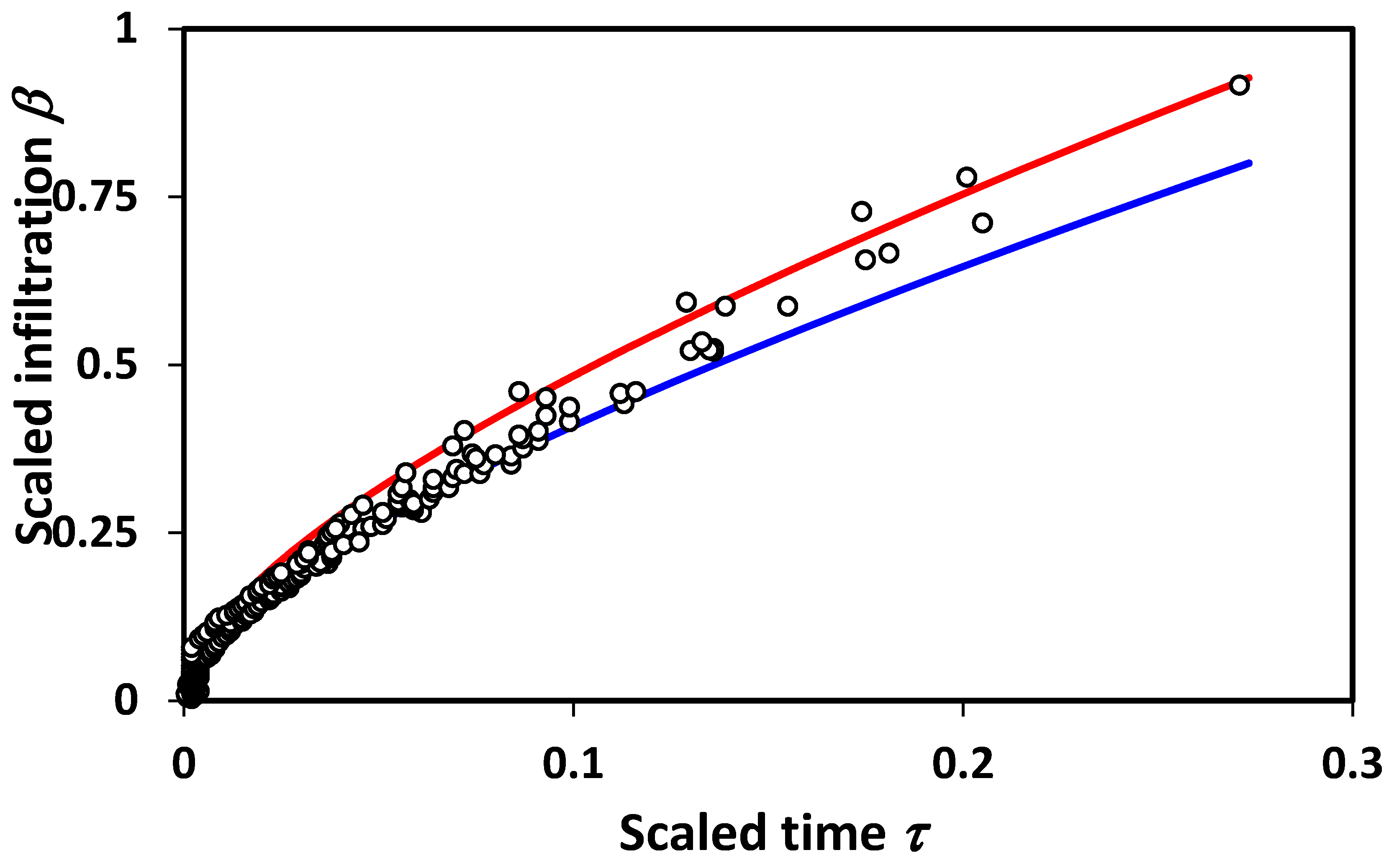
Perfect scaling, as predicted by Philip infiltration, is no longer quite developed, and a weak source of scatter is introduced (the factor
t00.04), generally in conformance with the results. However, in order to determine with certainty whether the residual scatter can be attributed to the additional time factor produced by our particular theoretical description, it would be necessary to know the individual values of
t0. Unfortunately, these values are not obtainable from the published data. It is clear, however, that the deviation must be due to a discrepancy in the power, because the formulation of the scaling functions [
32] eliminates any scatter due to variability in the coefficients. For a first estimate of how much uncertainty is introduced by the factor
t00.04, note that
t0 is proportional to
τ−1.06. From this, we estimate the variability in
t0 using the largest and smallest
τ values in the data set, 0.271 and 5.8 × 10
−4, respectively, providing minimum and maximum multiplicative factors of 1.05 and 1.32. Multiplication of the second term by these values gives the lower and upper bounds, respectively, on the theoretical prediction in
Figure 3. It should be noted finally that additional terms in the infiltration treatment due to Philip would also generate deviations in scaling. Interestingly, however, our lowest order theoretical treatment appears to generate just the right magnitude of scaling deviations to be compatible with experiment.
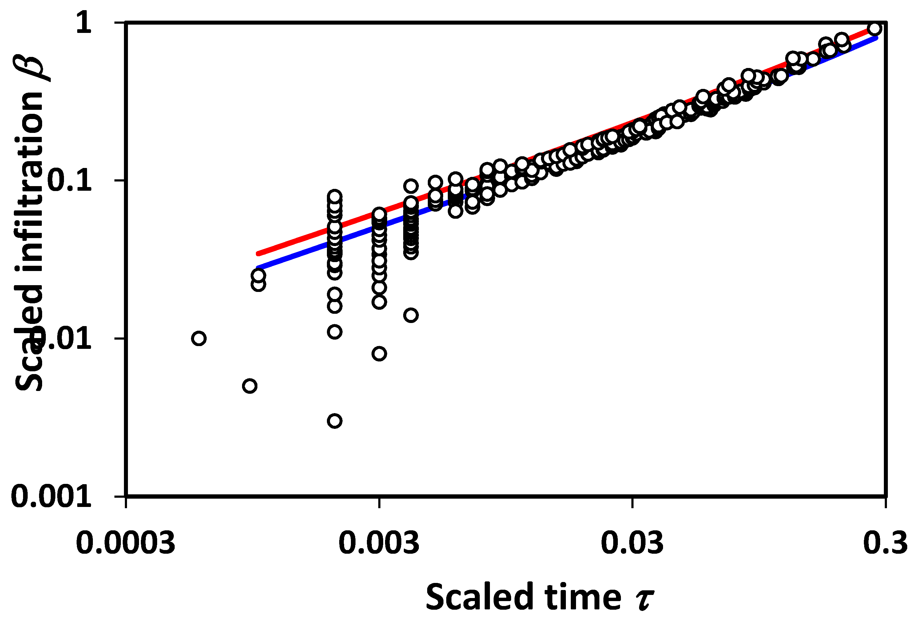
An important point relates to the limits of applicability of percolation techniques. For very short time scales, or equivalently, very small systems, fluctuations associated with the statistical variability introduced by small system sizes will produce a wide variability in results, and, typically, overestimate the infiltration (
Figure 3), while underestimating the mean [
19]. In accord with these observations, we reproduce in
Figure 4 a bi-logarithmic plot of the data and predictions given in
Figure 3. The results are in accord with the statistical interpretation, and with previous numerical results [
19] for the finite-size scaling of the hydraulic conductivity,
K, which similarly had a few values of
K that are much higher than predicted, and a larger number that are much lower (
Figure 4). This general conclusion is also in accord with the treatment of solute transport [
54], for which the simple scaling result underestimated the variability in solute dispersion at shorter distance scales, requiring calculation of the entire solute arrival time distribution for quantitative agreement with the experiment. If infiltration is analogous, the corresponding treatment of unsteady flow could introduce pore-size distribution effects into the short time (or distance) predictions.
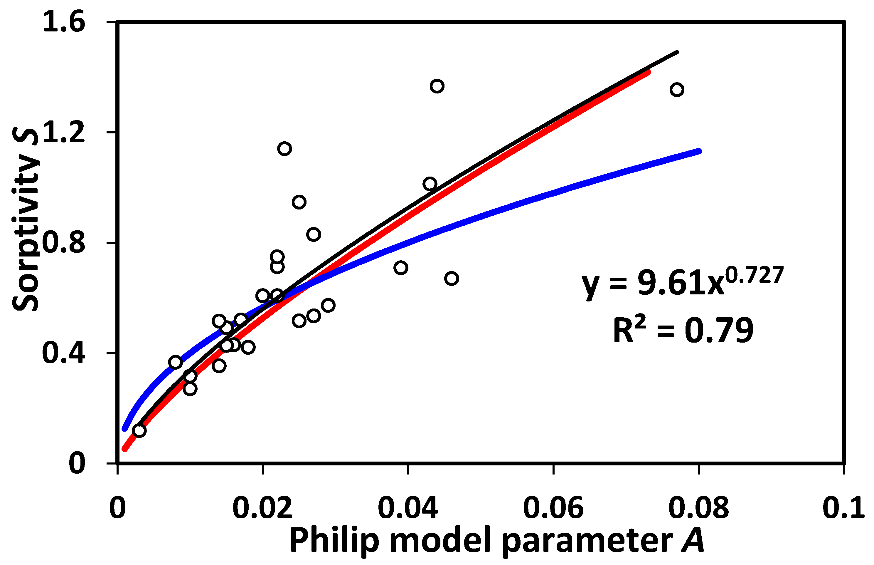
Finally, to confirm the accuracy of our above postulate, we test in
Figure 5 the prediction in [
32] regarding the relationship between
A and
S. Fitting of the data into a power-law form yields the relationship
S ~
A0.727, which is in reasonably good agreement with our prediction in the discussion following Equation (8) (0.77, 6% difference), but deviates significantly (by 45%) from the value predicted by the classical Philip’s infiltration theory, 0.5.

