Machine Learning Algorithms for the Forecasting of Wastewater Quality Indicators

Abstract

Stormwater runoff is often contaminated by human activities. Stormwater discharge into water bodies significantly contributes to environmental pollution. The choice of suitable treatment technologies is dependent on the pollutant concentrations. Wastewater quality indicators such as biochemical oxygen demand (BOD₅), chemical oxygen demand (COD), total suspended solids (TSS), and total dissolved solids (TDS) give a measure of the main pollutants. The aim of this study is to provide an indirect methodology for the estimation of the main wastewater quality indicators, based on some characteristics of the drainage basin. The catchment is seen as a black box: the physical processes of accumulation, washing, and transport of pollutants are not mathematically described.Two models deriving from studies on artificial intelligence have been used in this research: Support Vector Regression (SVR) and Regression Trees (RT). Both the models showed robustness, reliability, and high generalization capability. However, with reference to coefficient of determination R² and root-mean square error, Support Vector Regression showed a better performance than Regression Tree in predicting TSS, TDS, and COD. As regards BOD₅, the two models showed a comparable performance. Therefore, the considered machine learning algorithms may be useful for providing an estimation of the values to be considered for the sizing of the treatment units in absence of direct measures.

1. Introduction

In a rapidly developing world, water is more and more extensively polluted [1]. Urban areas can pollute water in many ways. Modifications of the urban environment lead to changes in the physical and chemical characteristics of urban stormwater [2]. The increase of impervious surfaces affects many components of the hydrologic cycle altering the pervious interface between the atmosphere and the soil. Runoff is heavily contaminated by pollution arising from industrial activities, civil emissions, and road traffic emissions. Stormwater collected in sewer systems and then discharged into water bodies significantly contributes to environmental pollution.

The selection of suitable wastewater treatment technologies needs an understanding of the pollutant concentrations. The stormwater quality characterization [3] is a challenging issue that has become of utmost importance with the increasing urban development. The problem complexity is mainly due to the randomness of the phenomena that govern the dynamics of pollutants in the basin and into the drainage network. The complexity is increased by the real difficulty of acquiring sufficient information to describe in detail the evolution of the pollution parameters during runoff.

The water quality in the sewer system during rain events depends on many factors related to the basin, the drainage system, the rainfall and, more generally, the climate.

The urban water pollution may be considered as consisting of four main processes:

-

Accumulation of sediments and pollutants on basin surface (build-up);

-

Washing of the surfaces operated by rain (wash-off);

-

Accumulation of sediments in the drainage system;

-

Transport of pollutants in the drainage system.

These phenomena can be modeled according to different approaches and the quality models may be used for different purposes in the study of urban runoff. In particular, the quality models are extremely useful for the characterization of effluents, the determination of the pollution load in the receiving watercourses, the evaluation of the dissolved oxygen in the flow [4], and the prediction of the effects of the drainage networks control systems.

Wastewater Quality Indicators (WQIs) give a measure of the physical (i.e., solid content, temperature, and electric conductivity), chemical (i.e., BOD₅, COD, total nitrogen, phosphate, heavy metals pH, and dissolved oxygen), and biological (pathogenic microorganisms, etc.) parameters in the effluents.

In order to choose the most appropriate treatment systems, the most used WQIs are biochemical oxygen demand (BOD₅), chemical oxygen demand (COD), total suspended solids (TSS), and total dissolved solids (TDS). These indicators are evaluated by means of specific laboratory tests.

TDS are measured as the mass of the solid residue remaining in the liquid phase after filtration of a water sample. Conversely, the mass of solids remained on the filter surface is the amount of TSS.

COD is used to indirectly measure the amount of reduced organic and inorganic compounds in water. Conversely, BOD₅ is the amount of dissolved oxygen needed by aerobic microorganisms to oxidize the biodegradable organic material present in the wastewater at a certain temperature in five days.

Wastewater treatment plants should be designed and sized using quality parameters (i.e., BOD₅, COD, TSS, and TDS) measured on samples taken from the influent wastewater, ideally in both dry and runoff conditions.

However, the direct measurements are often not available as the sampling of the wastewater cannot be performed. Therefore, the quality parameters are typically calculated by standard values of per capita production [5]. For instance, the influent BOD₅ is calculated assuming that each person produces 60 g O₂ per day.

This approach is reliable only when calculating the quality parameters under dry climate conditions. A method to estimate the influent quality parameters during runoff is therefore needed for properly sizing the wastewater treatment units.

Hence, the aim of this study is to provide an indirect methodology for the estimation of the main wastewater quality indicators, based on some characteristics of the drainage basin. The catchment is seen as a black box, with the physical processes of accumulation, washing, and transport of pollutants not mathematically described in detail.

Recently, models derived from artificial intelligence studies have been increasingly used in hydraulic engineering issues. Many researchers have investigated the feasibility of solving different water engineering problems, using Support Vector Regression (SVR) or Regression Trees (RT).

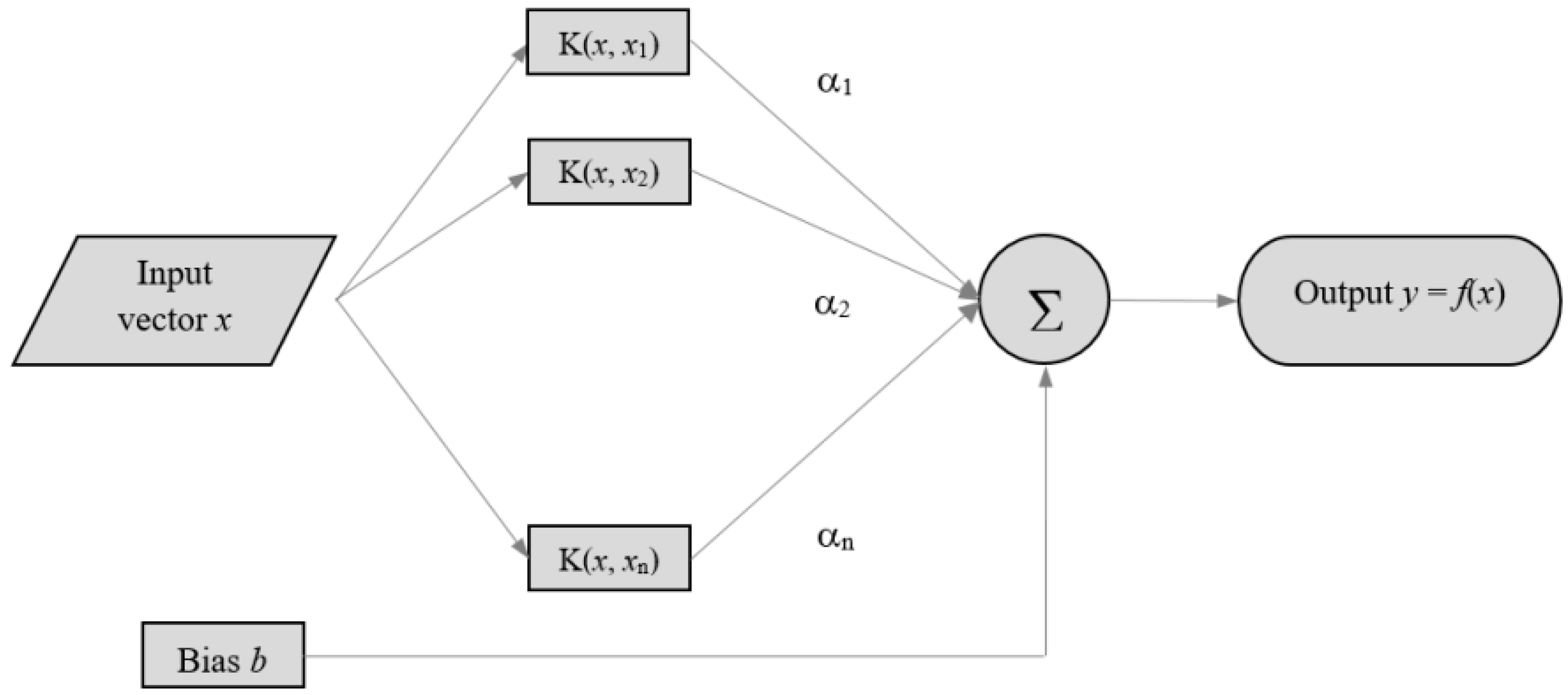
Support Vector Regression is a variant of Support Vector Machine, a machine-learning algorithm based on a two-layer structure. The first layer (Figure 1) is a kernel function weighting on the input variable series, while the second is a weighted sum of the kernel outputs.

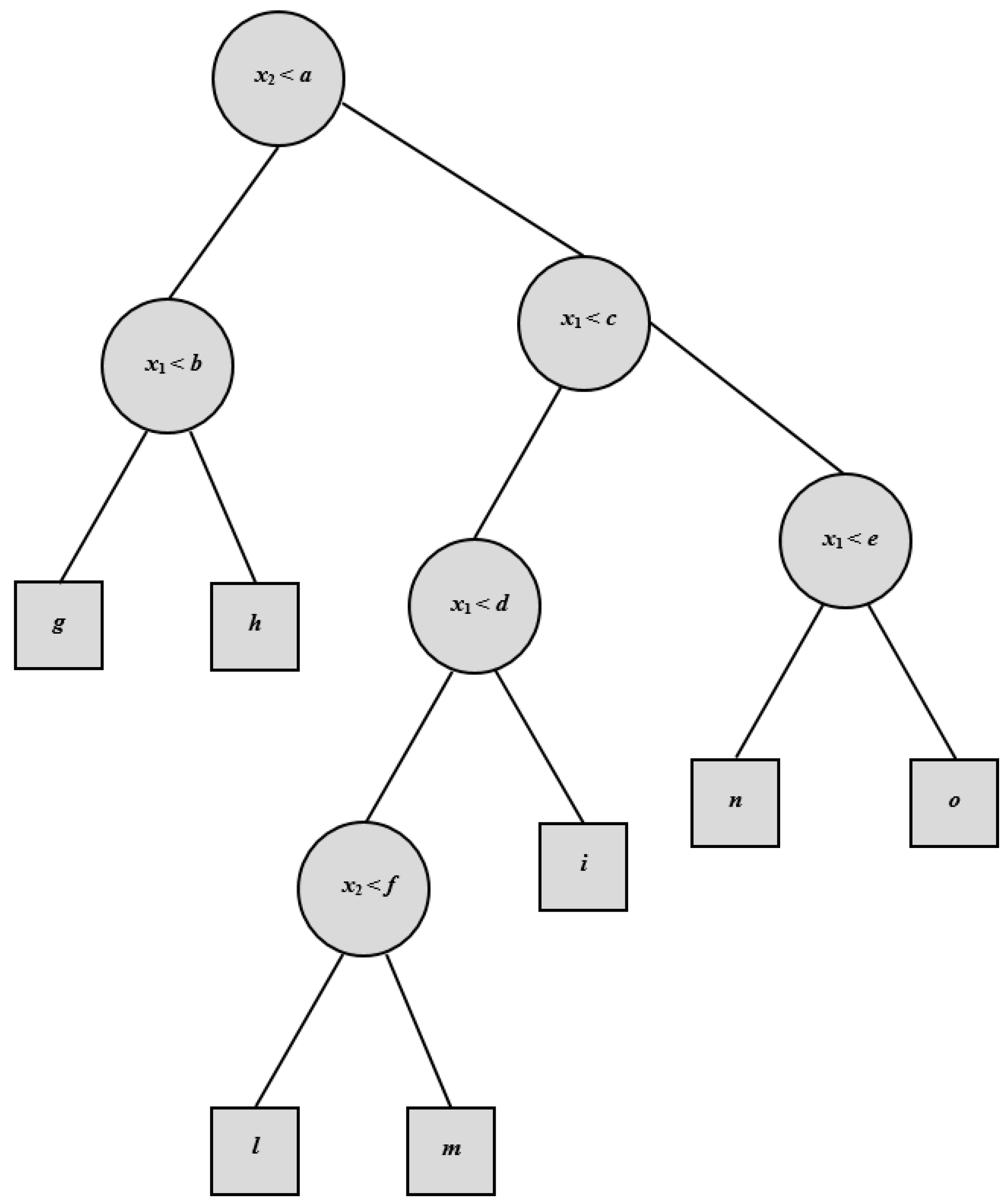
Regression Tree analysis is based on a decision tree that is used as a predictive model (Figure 2). The tree is obtained by splitting the source set into subsets on the basis of an attribute value test. The process is recursively repeated on each derived subset. It reaches a conclusion when the subset at a node has all the same values of the target variable, or when splitting no longer improves the results of the predictions.

Dibike et al. [6] used Support Vector Machines in rainfall-runoff modeling in comparison with ANN models. Bray and Han [7] emphasized the difficulties in identifying a suitable model structure and the parameters for the rainfall-runoff modeling. Chen et al. [8] applied SVMs to forecast the daily precipitation in the Hanjiang basin. Granata et al. [9] performed a comparative study of rainfall-runoff modeling between a SVR-based approach and the EPA’s Storm Water Management Model. Raghavendra and Deka [10] provided an extensive review of the SVM applications in hydrology.

The RT method has been employed for sediment transport [11,12], flood prediction [13], mean annual flood forecasting [14], scour depth prediction [15,16], and sediment yield estimation in rivers [17].

A comparative study of the wastewater quality modeling between a Support Vector Regression and Regression Tree-based approaches has been performed in this work. The experimental data was taken from the National Stormwater Quality Database (NSQD), and developed under the support of the U.S. Environmental Protection Agency [18]. The water quality indicators have been correlated to the main characteristics of the basin, such as the drainage area, the percentage of impervious surface, the types of land use, the height of rain, and the surface runoff.

2. Materials and Methods

2.1. Support Vector Regression

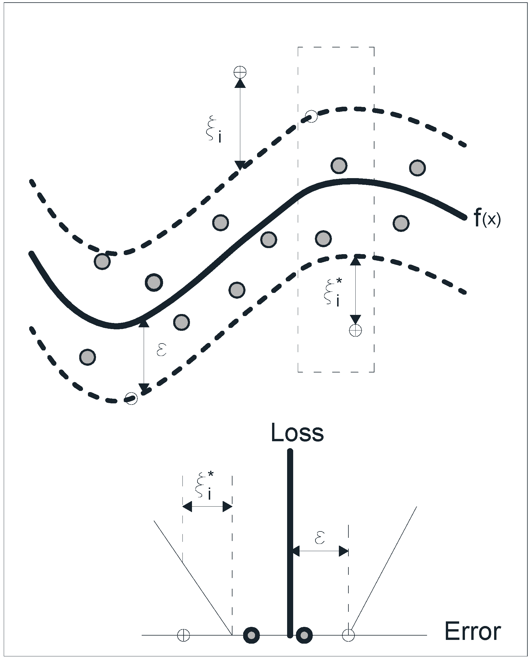
Support vector machines (SVMs) are supervised learning models that analyze data for classification or regression analysis (SVR). Given a training data set {(x₁, y₁), (x₂, y₂), …, (x_l, y_l)} ⊂ X × R, where X is the space of the input patterns (e.g., X = Rⁿ), in SVR the main aim is to find a function f(x) that is characterized by a maximum ε deviation from the actually obtained target values y_i for all the training data. Moreover, f(x) has to be as flat as possible.

The errors smaller than ε are tolerated, while the errors greater than ε are generally unacceptable. For this purpose, for linear functions in the form

$$f(x)=\langle w,x\rangle +b$$

(1)

in which w ∈ X, b ∈ R and $\langle \cdot ,\cdot \rangle$ is the dot product in X, the Euclidean norm ||w||² has to be minimized. Accordingly, the problem can be considered as a convex optimization problem, as reported in the following equations:

$$\begin{array}{c}\text{minimize} \frac{1}{2}{\Vert w\Vert }^2\\ \text{subject to} \{\begin{array}{l}{y}_i-\langle w,x_i\rangle -b\le \epsilon \\ \langle w,x_i\rangle +b-y_i\le \epsilon \end{array}\end{array}$$

(2)

Equation (2) implicitly states that a function f is capable of approximating all the pairs (x_i, y_i) with ε precision. However, in many cases this is not possible, or a certain error has to be tolerated. Therefore, slack variables ξ, ξ${ }_i^{*}$ have to be introduced (Figure 3) in the constraints of the optimization problem, based on the following formulation:

$$\begin{array}{c}\text{minimize} \frac{1}{2}{\Vert w\Vert }^2+C{\displaystyle \sum _{i=1}^l\left({\xi }_i+{\xi }_i^{*}\right)}\\ \text{subject} \text{to} \{\begin{array}{l}{y}_i-\langle w,x_i\rangle -b\le \epsilon +{\xi }_i\\ \langle w,x_i\rangle +b-y_i\le \epsilon +{\xi }_i^{*}\end{array}\end{array}$$

(3)

Both the flatness of f and the accepted deviations larger than ε depend on the constant C > 0. The optimization problem defined in Equation (3) is commonly solved in its dual formulation, utilizing Lagrange multipliers:

$$L=\frac{1}{2}{\Vert w\Vert }^2+C{\displaystyle \sum _{i=1}^l\left({\xi }_i+{\xi }_i^{*}\right)-{\displaystyle \sum _{i=1}^l{\alpha }_{\mathrm{i}}\left(\epsilon +{\xi }_i-y_i+\langle w,x_i\rangle +b\right)-}}{\displaystyle \sum _{i=1}^l{\alpha }_i^{*}\left(\epsilon +{\xi }_i^{*}+y_i-\langle w,x_i\rangle -b\right)-}{\displaystyle \sum _{i=1}^l\left({\eta }_i{\xi }_i+{\eta }_i^{*}{\xi }_i^{*}\right)}$$

(4)

in which ${\alpha }_i,{\alpha }_i^{*},{\eta }_i,{\eta }_i^{*}\ge 0$, whereas the partial derivatives of L with respect to the variables $\left(w,b,{\xi }_i{\xi }_i^{*}\right)$ must be equal to zero in the optimal condition.

Thus, the dual optimization problem can be formulated as

$$\begin{array}{c}\text{maximize} \{\begin{array}{l}-\frac{1}{2}{\displaystyle \sum _{i,j=1}^l}\left({\alpha }_i-{\alpha }_i^{*}\right)\left({\alpha }_j-{\alpha }_j^{*}\right)\langle x_i,x_j\rangle \\ -\epsilon {\displaystyle \sum _{i=1}^l}\left({\alpha }_i+{\alpha }_i^{*}\right)+{\displaystyle \sum _{i=1}^l}{y}_i\left({\alpha }_i-{\alpha }_j^{*}\right)\end{array}\\ \text{subject to} \{\begin{array}{l}{\displaystyle \sum _{i=1}^l}({\alpha }_i-{\alpha }_i^{*})=0\\ {\alpha }_i,{\alpha }_i^{*}\in [0,C]\end{array}\end{array}$$

(5)

The calculation of b can be performed on the basis of the Karush-Kuhn-Tucker conditions [19] which impose that the product between constraints and dual variables must vanish at the optimal solution, that is:

$$\begin{array}{l}{\alpha }_i\left(\epsilon +{\xi }_i-y_i+\langle w,x_i\rangle +b\right)=0\\ {\alpha }_i^{*}\left(\epsilon +{\xi }_i^{*}+y_i-\langle w,x_i\rangle -b\right)=0\end{array}$$

(6)

and

$$\begin{array}{l}\left(C-{\alpha }_i\right){\xi }_i=0\\ \left(C-{\alpha }_i^{*}\right){\xi }_i^{*}=0\end{array}$$

(7)

Then, in order to make the Support Vector algorithm nonlinear, the training patterns x_i can be preprocessed by a map Φ: X → F, where F is some feature space. The SVR algorithm is only depending on the dot products between the various patterns, making sufficient use of a kernel $k(x_i,x_j)=\langle \mathsf{\Phi }(x_i),\mathsf{\Phi }(x_j)\rangle$ instead of the map Φ(∙) distinctly. Hence, the Support Vector algorithm can be rewritten as:

$$\begin{array}{l}\mathrm{maximize}\{\begin{array}{l}-\frac{1}{2}{\displaystyle \sum _{i,j=1}^l}\left({\alpha }_i-{\alpha }_i^{*}\right)\left({\alpha }_j-{\alpha }_j^{*}\right)k\left(x_i,x_j\right)\\ -\epsilon {\displaystyle \sum _{i=1}^l}\left({\alpha }_i+{\alpha }_i^{*}\right)+{\displaystyle \sum _{i=1}^l}{y}_i\left({\alpha }_i-{\alpha }_j^{*}\right)\end{array}\\ \mathrm{subject\; to}\{\begin{array}{l}{\displaystyle \sum _{i=1}^l}({\alpha }_i-{\alpha }_i^{*})=0\\ {\alpha }_i,{\alpha }_i^{*}\in [0,C]\end{array}\end{array}$$

(8)

The expansion of f can be formulated as follows:

$$f(x)={\displaystyle \sum _{i=1}^l\left({\alpha }_i-{\alpha }_i^{*}\right)}k(x_i,x)+b$$

(9)

Although uniquely defined, w is no longer explicitly identified, unlike in the linear case. In the nonlinear case, the optimization problem is to find the flattest function in the feature space, not in the input space. The Mercer’s condition has to be satisfied for the functions k(x_i, x_j), which corresponds to a dot product in some feature space F [20].

In this study, a radial basis function (RBF) has been chosen as kernel. The RBF has the form:

$$k(x_i,x_j)=\exp \left(-\gamma {\Vert x_i-x_j\Vert }^2\right),\gamma >0$$

(10)

A Support Vector algorithm was implemented in the MATLAB environment. The search for the optimal structure of the model and its parameters was conducted by means of a trial and error iteration procedure. The deviation between the function found by the SVR and the target value was controlled by the ε parameter. Finally, ε was chosen to be equal to 0.01, while the cost of error C, which affects the smoothness of the function, was assumed equal to 1.

2.2. Regression Tree

A Regression Tree [21] is a variant of Decision Trees, developed to approximate real-valued functions. Once again, the aim is to develop a model that can predict the value of a target variable, given several input variables. In the RT model, the whole input domain is recursively partitioned into sub-domains, while a multivariable linear regression model is used to make predictions in each of them. The tree is composed of a root node (containing all data), a set of internal nodes (splits), and a set of terminal nodes (leaves).

The building process of Regression Trees consists of an iterative process that splits the data into partitions or branches. Initially, all data in the training set is grouped in a single partition. The algorithm then starts to allocate the data into the first two branches, using every possible binary split on every field. Subsequently, the procedure continues splitting each partition into smaller groups, as the method moves up each branch. At each stage, the algorithm selects the split that minimizes the sum of the squared deviations from the mean in the two separate partitions.

The process is repeated until each node reaches a user-specified minimum node size, becoming a terminal node. If the sum of squared deviations from the mean tends to zero in a node, then it is considered a terminal node even if the minimum size has not been reached.

In other words, for each node the algorithm selects the partition of data that leads to nodes ‘purer’ than their parents. The process stops if the lowest impurity level is reached or if some stopping rules are met. These stopping rules are generally associated with the maximum tree depth (i.e., the final level reached after successive splitting from the root node), the minimum number of units in nodes, or the threshold for the minimum variation of the impurity provided by new splits.

In the RT algorithm, the impurity of a node is evaluated by the Least-Squared Deviation (LSD), R(t), which is simply the within variance for the node t:

$$R(t)=\frac{1}{N(t)}{\displaystyle \sum _{i\in t}{(y_i-y_m(t))}^2}$$

(11)

in which N(t) is the number of sample units in the node t, y_i is the value of the response variable for the i-th unit, and y_m is the mean of the response variable in the node t.

The function of the Least-Squared Deviation criterion for split s at the node t may be defined as follows:

$$\varphi (s,t)=R(t)-p_{L}R(t_L)-p_{R}R(t_R)$$

(12)

where t_L and t_R are the left and right nodes generated by the split s, respectively, while p_L and p_R are the portions of units assigned to the left and right child node. The split s that maximizes the value of $\varphi (s,t)$ is finally chosen, subsequently providing the highest improvement in terms of tree homogeneity.

Since the tree is built from training samples, it might suffer from over-fitting when the full structure is reached. This may deteriorate the accuracy of the tree when applied to unseen data and lead to a lower generalization capability.

For this reason, a pruning process is often used in order to obtain an optimal dimension tree. This process is defined as Error-Complexity Pruning: after the tree generation, the process removes the redundant splits of the tree. Concisely, this method is based on a measure of both error and complexity, depending on the number of nodes, for the generated binary tree. An accurate description of the pruning algorithm is reported by Breiman et al. [21].

2.3. The Database

The data of the NSQD was collected by the University of Alabama and the Center for Watershed Protection, funded by the U.S. Environmental Protection Agency (EPA). The monitoring period of the used data is from 1992 to 2002. The NSQD contains about 3765 events from 360 sites in 65 communities in the U.S.A. [18]. The drainage area of the considered basins ranges from about 0.16 hectares to more than 1160 hectares.

For each site the database also includes additional information, such as the geographical location, the total area, the percentage of impervious cover, the percentage of each land use in the catchment. In addition, the characteristics of each event such as total precipitation, precipitation intensity, total runoff, and antecedent dry period are also included. It is important to highlight that the database only contains information for samples collected at drainage system outfalls, while in-stream samples were not included.

3. Results and Discussion

As the database was widely incomplete with regard to many sets of data, it was possible to use only a part of them. The input matrix for both models consisted of a series of vectors containing the following quantities: drainage area, percentage of residential area, percentage of institutional area, percentage of commercial area, percentage of industrial area, percentage of open space area, percentage of freeway, percentage of impervious area, precipitation depth, and runoff.

The training and testing dataset size of the two prediction models, for each of the four considered indicators, is shown in

Table 1. Training and testing dataset size.

WQI	Training Dataset Size	Testing Dataset Size
TSS	811	50
TDS	894	44
COD	1108	42
BOD	680	40

. The difference in size is due to the different data availability.

The effectiveness of prediction algorithms was evaluated by two criteria: the root-mean square error (RMSE) and the coefficient of determination R². The latter is a number that indicates the proportion of the variance in the dependent variable that is predictable from the independent variable, giving some information about the goodness of fit of a model. It is defined as

$$R^2=\left(1-\frac{{\displaystyle {\sum }_{i=1}^m{\left(I_{pi}-I_{mi}\right)}^2}}{{\displaystyle {\sum }_{i=1}^m{\left(I_a-I_{mi}\right)}^2}}\right)$$

(13)

where m is the total number of measured data, I_pi is the predicted value of the considered water quality indicator for data point i, I_mi is the measured indicator for data point i, I_a is the averaged value of the measured values of the indicator. The root-mean square error represents the sample standard deviation of the differences between predicted and observed values. It is defined as:

$$\mathrm{RMSE}=\sqrt{\frac{{\displaystyle {\sum }_{i=1}^m{\left(I_{pi}-I_{mi}\right)}^2}}{m}}$$

(14)

It aggregates the magnitudes of the errors in predictions into a single measure of predictive power.

Table 2. Comparison between SVR and RT by means of RMSE and R².

	RMSE (mg/L)		R2
WQI	SVR	RT	SVR	RT
TSS	1049	3486	0.97	0.906
TDS	1549	1826	0.851	0.828
COD	1172	2395	0.893	0.784
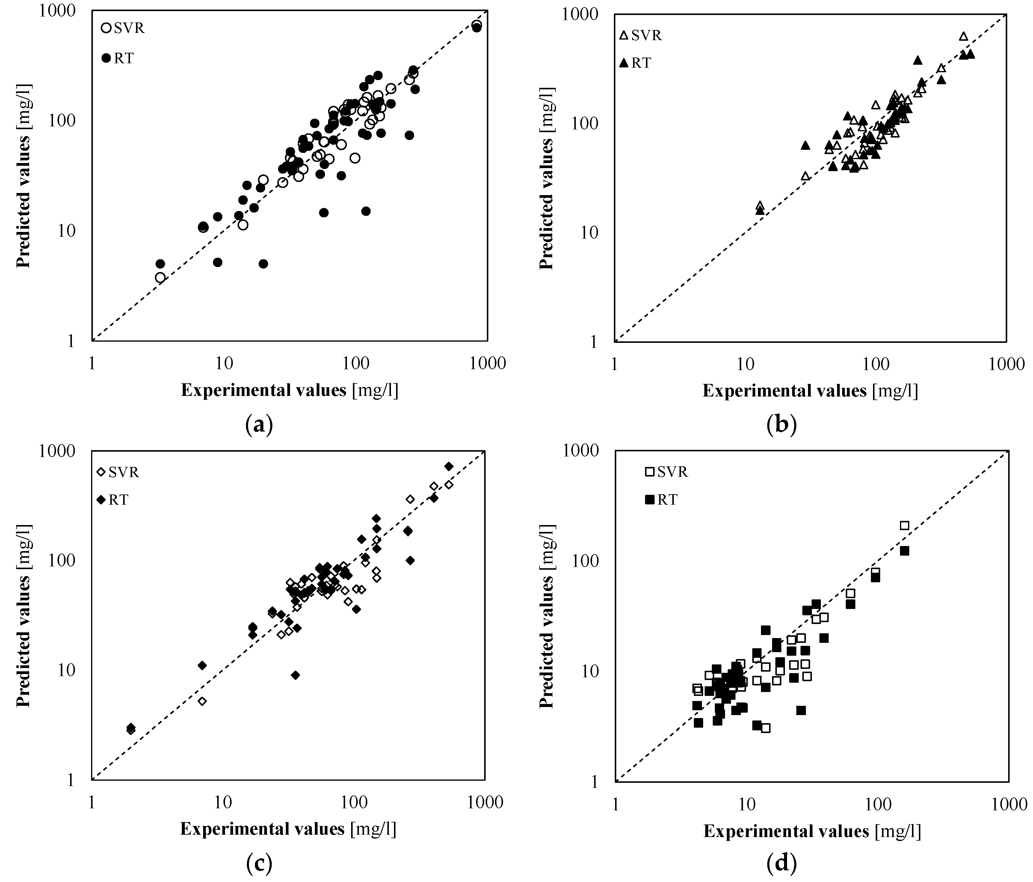
BOD	104	103	0.87	0.871

and Figure 4 show that both models are able to provide good predictions of water quality parameters. The analysis of RMSE shows that the SVR model was characterized by a better accuracy in predictions of TSS, TDS, and COD than the RT model (Table 2). The difference was particularly relevant with regard to TSS and COD. As regards the BOD₅, instead, the two models showed a similar performance.

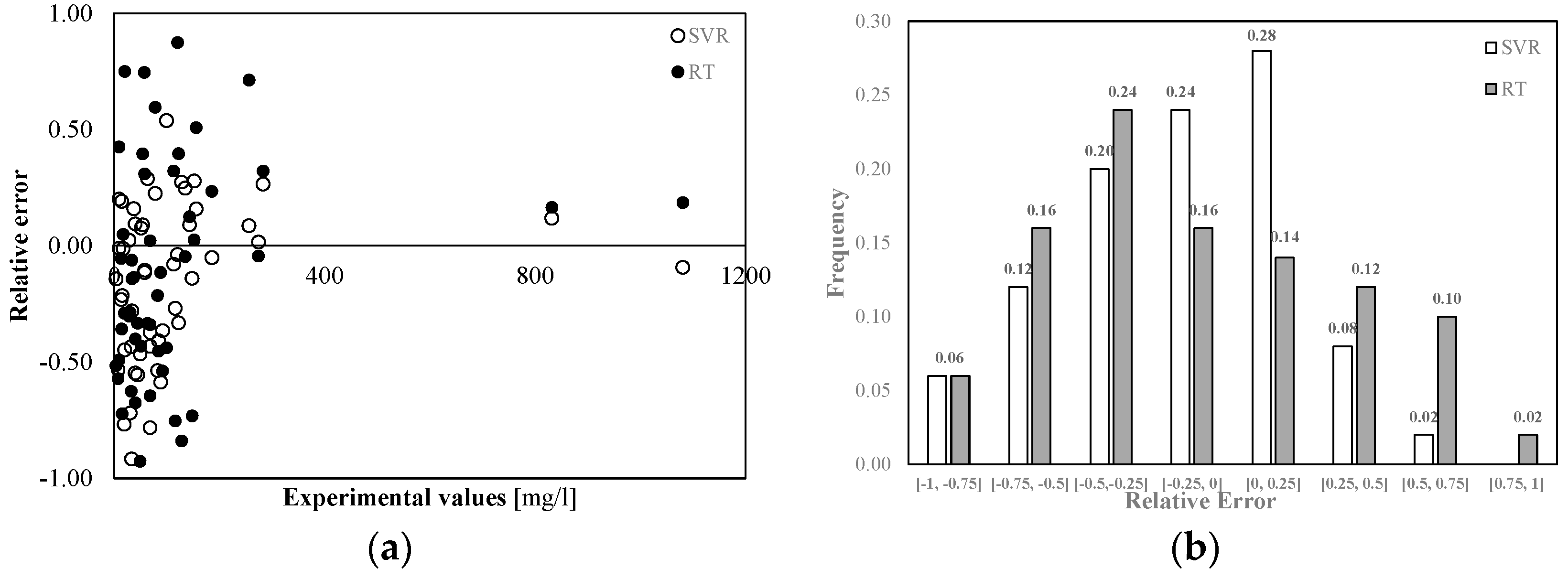
Figure 5 shows the relative error distribution in the TSS predictions made with both models. The highest relative errors were observed in correspondence of the lowest measured values, while in correspondence of the highest experimental values, the relative error was less than 0.2. The use of Regression Tree led to generally higher errors. From Figure 5b it can be seen that 50% of the results provided by SVR were affected by an error less than 25% in absolute value, while only 30% of the results provided by RT were characterized by a less than 25% error. In addition, 62% of the results provided by the two models suffered from a negative relative error. Both SVR and RT showed a clear tendency to overestimate the experimental data.

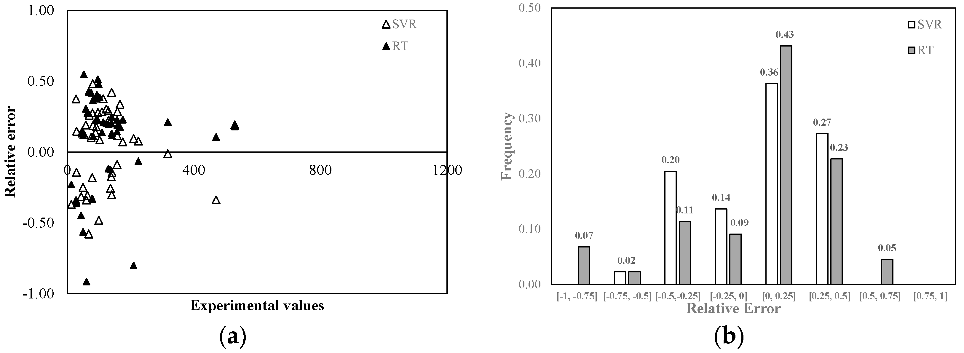
Figure 6 shows the relative error distribution in the TDS tests. The highest relative errors were found for the TDS values between 0 and 200 mg/L. From Figure 6b, it can be seen that 50% of the results provided by SVR were affected by a less than 25% error in absolute value, while 52% of the results provided by RT were characterized by a less than 25% error. However, the highest errors were made by using a Regression Tree. 14% of the results provided by RT was affected by an error greater than 50%, while only 2% of the results provided by SVR had such a large error. Moreover, 71% of the results obtained with RT and 63% of those obtained with SVR showed a positive relative error: both algorithms tended to underestimate the experimental results.

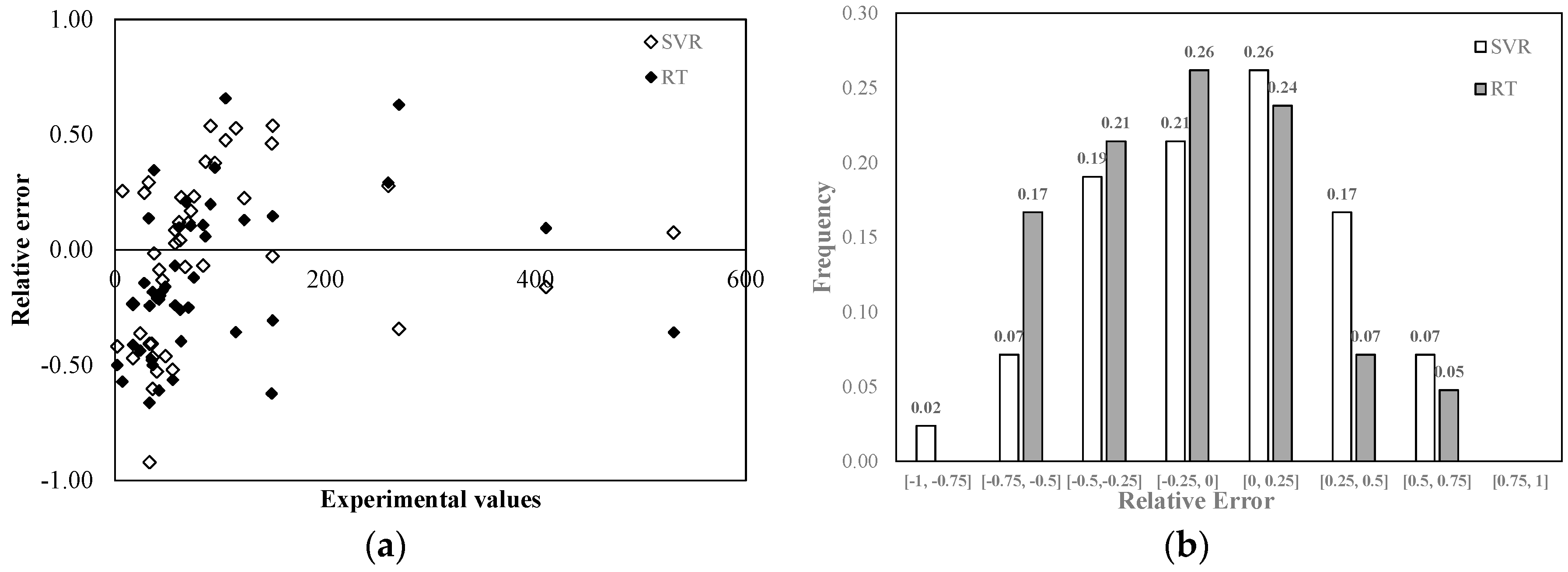
Relative error distributions in the COD predictions made with both models are shown in Figure 7. Again, the highest relative errors were observed in correspondence of the lowest measured values, while in correspondence of the highest experimental values, the relative error was quite small: less than 10% in the case of SVR was approximately equal to 30% for RT.

Figure 7b shows that 47% of the results provided by Support Vector Regression were affected by a less than 25% error in absolute value, while 50% of the results provided by Regression Tree were characterized by a less than 25% error. Furthermore, relative errors were equally distributed around zero in the case of SVR, while 64% of the results provided by RT showed a negative relative error and a tendency to overestimate the experimental results.

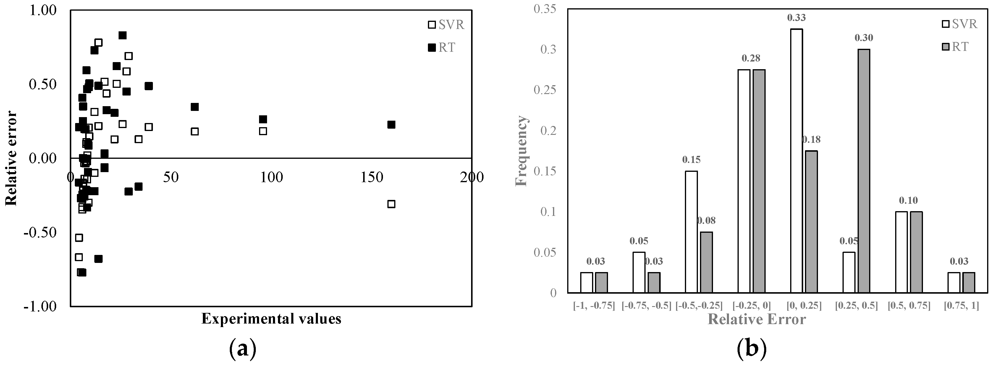
Figure 8 shows the relative error distribution in the BOD₅ tests. In this case, the highest relative errors were found for the BOD₅ values between 0 and 50 mg/L. In correspondence of the highest measured values the relative error was less than 25% for both models. From Figure 8b, it may be noticed that 61% of the results provided by SVR was affected by a less than 25% error in absolute value, while 46% of the RT outcomes showed a less than 25% error. In addition, SVR leads to equally distributed errors around zero, while RT showed a tendency to underestimate the experimental results.

The considered machine learning algorithms were characterized by robustness and reliability. Both the models proved to be able to provide good predictions of the WQI values in very different situations as regards basin characteristics and rainfall events.

The obtained results highlight that the proposed modelling approaches are able to produce formulations with a high generalization capability. Therefore, machine learning based models are a valuable alternative to the physically based modelling in the forecasting situations. This is particularly emphasized when the physical processes are difficult to identify and formulate in a suitable mathematical form. Data driven models naturally try to minimize the dependency on knowledge of the real-world processes.

However, machine-learning algorithms suffer from some significant limitations. An optimal buildup of the model is often a complex procedure. In addition, a selection of inadequate variables can deteriorate the model performance. Finally, a reliable model training needs a large set of events, including samples of the typical situations that may occur in simulation scenarios. The use of limited samples of training data may result in poor quality of predictions.

4. Conclusions

An indirect methodology for the estimation of the main effluent quality parameters was tested in this study. The methodology accounts the following characteristics of the urban catchment: drainage area, percentage of residential area, percentage of institutional area, percentage of commercial area, percentage of industrial area, percentage of open space area, percentage of freeway, percentage of impervious area, precipitation depth, and runoff.

Two different machine-learning algorithms were compared: Support Vector Regression and Regression Tree. Both the models showed robustness, reliability, and high generalization capability. However, with reference to root-mean square error and coefficient of determination R², Support Vector Regression showed a better performance than Regression Tree in forecasting TSS, TDS, and COD. As regards BOD₅, the two models showed a comparable performance.

Machine learning algorithms may be also useful for providing an estimation of the values to be considered for the sizing of the treatment units, given the characteristics of the basin, when direct measures are not available.

The proposed approach could also be effective in the context of the real-time management issues of the wastewater treatment plants, as well as used to address environmental planning issues.