Effects of Different In-Stream Structure Representations in Computational Fluid Dynamics Models—Taking Engineered Log Jams (ELJ) as an Example

Abstract

In-stream structures contribute greatly to the biodiversity in streams and play an important role in restoring and protecting rivers. They usually have complex geometries. To evaluate their impact and effectiveness, computational models are increasingly used. However, how to faithfully represent them in computer models remains a challenge. Often, simplifications have to be made. This work evaluated the effects of geometric simplification of an example in-stream structure, an engineered log jam (ELJ), in computational models. Three different representations were considered, namely full resolution, the porous media model and the solid barrier model. The turbulent flow was resolved with large eddy simulation (LES). First, the simulations were validated with a physical experiment in a flume. Then, the results from the three models were compared and analyzed on various aspects related to the stability and functionalities of the structures. Unsurprisingly, it is found that the porous media model and the solid barrier model, which are computationally economic, can describe the flow dynamics only to some extent. From the calibration of drag force and wake length, we found that the equivalent grain size $d_{50}$ in the porosity model should scale as the key element diameter for the simulated ELJ. A wake length scale analysis was performed for the semi-bounded flow around this in-stream structure near the bank. The length estimator in the literature for unbounded vegetation patches can be used with modifications. The results also show that the flow passing through the porous in-stream structure has a significant impact on mean velocity, turbulence kinetic energy, sediment transport capacity and integral wake length. Since geometrically-fully-resolved simulations are not currently feasible for engineering practices, the following suggestions are made based on this study. If the near-field and wake are important for the purpose of the structure, the well-calibrated porosity model seems to perform better than the solid barrier model. However, care needs to be taken when interpreting the results because this work also identified substantial loss of physical information with the porosity model. When the emphasis is the far field away from the structure, both the porosity model and the solid barrier model give comparable results.

1. Introduction

In-stream structures have been used widely in engineering practice for various purposes, e.g., river training, channel stabilization, erosion control and habitat restoration. In the past several decades, the science and engineering communities have gradually realized that Mother Nature provides great examples of good in-stream structures, which serve multiple purposes. One such natural structure is large woody debris (LWD), which consists of fallen trees, stumps and root-wads, with irregular and complex geometries. Their ecological significance has been recognized since the 1980s [1,2,3]. Studies have found that LWD greatly increases stream habitat complexity [4]. Organic matter can easily accumulate in-between the debris of snags, leaves and root-wads, which provides nutrients and food for living organisms. The debris structures were reported to contain more than half of the organic matter in lower-order streams [5], which provides abundant food sources for invertebrates, fishes and macro-invertebrate biomass. The structures can also function as shelters for fishes and prevent them from being attacked by predators [6]. The slow flow region in the wake of in-stream structures provides a resting area and helps fish regain energy [7]. The ecological benefits of in-stream structures highly rely on the hydrodynamics within and around them. Recognizing their importance to rivers, in-stream structures have been widely used in stream restoration projects [8]. Examples of these structures include single log vane, log cross vane, mud sill, multi-log vane deflector, water jack and engineered log jams (ELJ) [9], among which ELJ is a very attractive option due to its abundant eco-hydraulic benefits [10].

The proper design of in-stream structures depends on the understanding of the associated hydraulics. These in-stream structures can be regarded as roughness elements in rivers. They alter the flow conditions by slowing down surrounding flow and changing local water depths [11]. In the measurements of Cultus River, Manga et al. [12] found that LWD, which only covered 2% of flow area, contributed half of the total flow resistance in the stream. A recent flume study also showed that if these structures are fixed, they can delay the flooding time and significantly lower the runoff coefficient, which helps reduce erosion and suppress flooding damage [13]. Thus, one important design parameter is the flow resistance due to LWDs. On the other hand, the drag force experienced by the structures is an important factor for their stability.

There are two major methods to quantify the flow resistance due to in-stream structures. The first one is to use the concept of stress partitioning, which was first introduced for the study of fluvial dynamics [14]. This method separates the flow resistance due to debris from the total. For example, some researchers created new Darcy–Weisbach friction factors for the prediction of flow resistance in the stream, which is constituted of bed shear, bend curvature and drag from debris [12,15,16]. In this method, it is critical yet difficult to estimate the debris drag coefficient. It is often observed that LWDs contain much sediment and many leaves inside the gaps between snags and root-wads. Therefore, these structures are treated as solid barriers, and as a result, simple theoretical models can be applied to calculate the drag force exerted on them [15]. In early studies, a very common approximation is to use a single cylinder as a proxy for a log in the streams. Flume experiments were conducted to investigate how the side-walls, bed bottom and orientation would affect the drag and lift coefficients for a single log [17,18,19].

Another method is to use the one-dimensional (1D) momentum equation to compute the drag force exerted on in-stream structures. For example, Turcotte et al. [20] found that the drag forces on large cylinders calculated from the momentum equation matched well with the measured values. They also found that the classic drag force formulas underestimate the force if the cylinder diameter is much larger than critical water depth. Compared with the stress partitioning method, the momentum analysis method is more applicable to complex and porous accumulations, like debris jams. For example, Manners et al. [21] measured detailed velocity around natural woody debris jams and calculated drag coefficients through the moment equation.

Numerous studies have shown the complexity of in-stream structures and the deviation of their hydraulic behavior from the predictions made by the two methods mentioned above. For example, Manners et al.’s [21] results show the drag coefficient for the debris jams ranges from 2.6 to 9.0. In contrast, the drag coefficient is about 0.8 for a cylinder and one for a cube. Manners et al.’s [22] field study indicates that for debris jams, the drag decreases as the porosity increases. A more recent study of Shields and Alonso [23] shows that the roughness on the surface of cylinder increases lift, but reduces wave force (which is the difference between actual drag force and theoretical drag force). They also found that the effect of surface roughness is not as significant as the bed proximity, blockage rate and submergence. However, under certain conditions, the increase of complexity may reduce the drag coefficient. Gippel et al.’s [19] flume study showed that branches added to a single trunk would lower the drag coefficient because the increase of drag force was less than the percentage increase of the frontal area.

For the solid barrier model in hydraulics, a very classic application of CFD is in the groyne fields [24,25]. The use of CFD to study the porous in-stream structures is rare in the fluvial hydraulics community. As an infrequent case in this point, in order to evaluate the geometric complexity of woody debris, computational simulations were performed by Allen et al. [26]. They developed a shape complexity factor to quantify the geometric complexity of LWD. Their simulations showed that both the drag coefficient and the integrated turbulence kinetic energy decrease with the complexity factor. However, for the complex and porous structures, it is very difficult to compute the shape complexity factor. There are more CFD studies in coastal engineering for coastal structures, which often consist of amour rocks [27,28]. In order to simplify the simulations, these coastal engineering studies usually adopt a porous media flow model by adding resistance source terms, which are calculated with an extended Darcy–Forchheimer equation, into the Navier–Stokes equations. Jensen et al. [29] calibrated the empirical resistance coefficients for coastal structures. Their simulation results had a good match with the experimental data. A similar porosity model will be evaluated in this study.

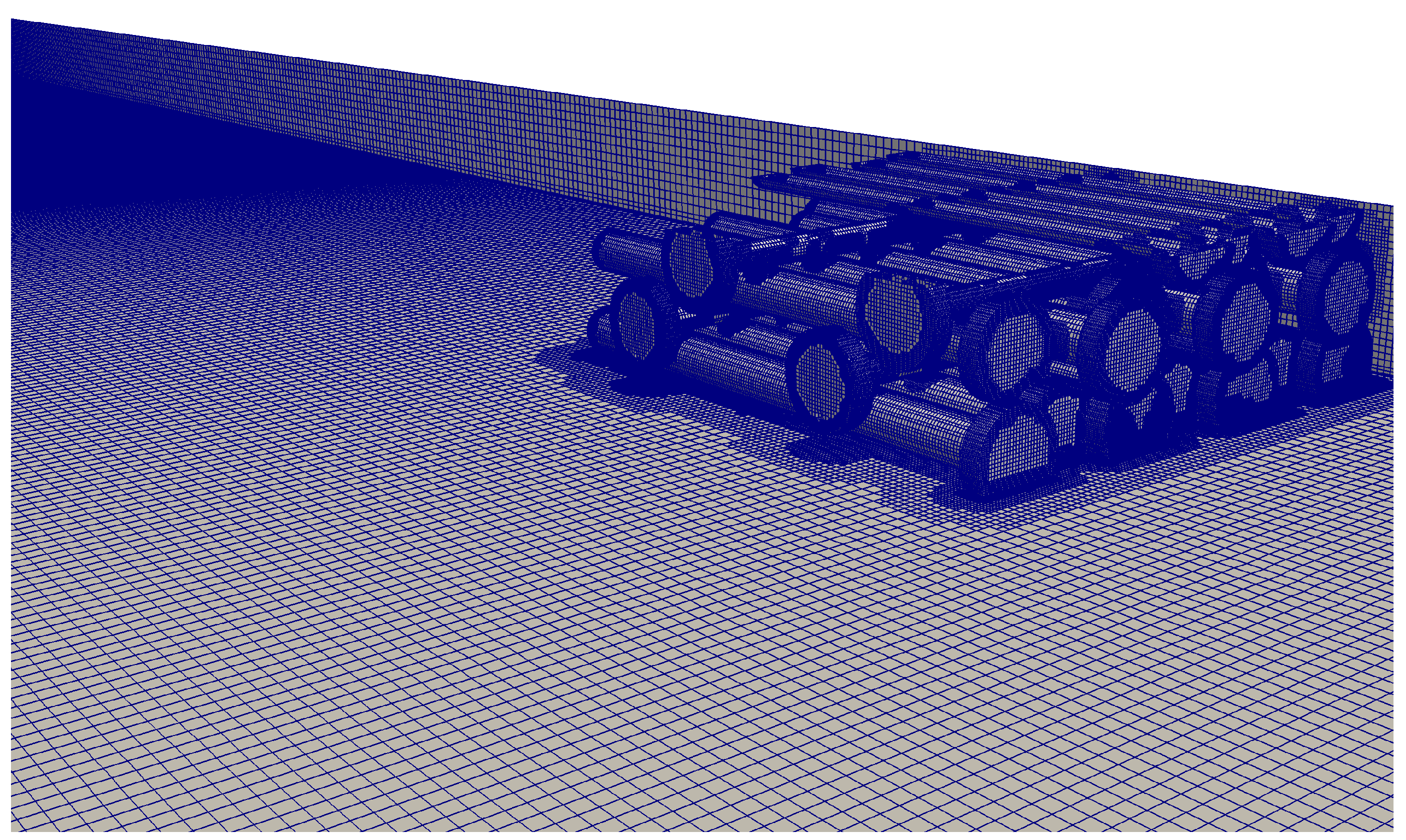
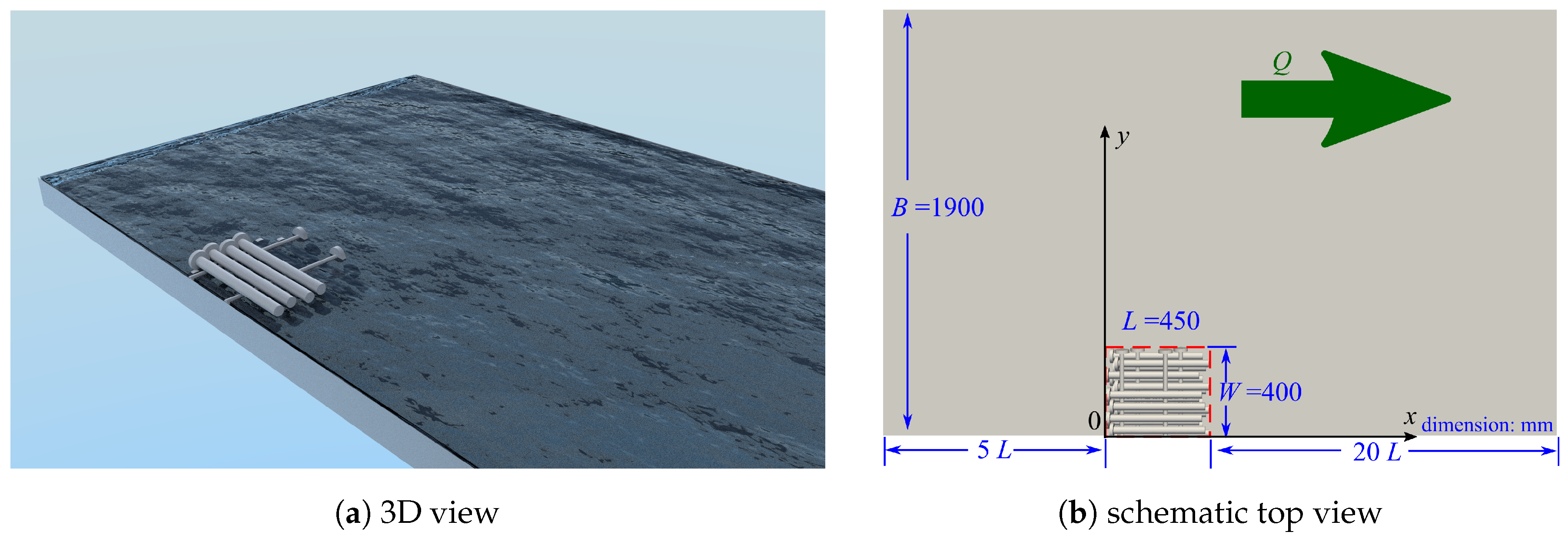
This paper presents the findings on the effects of different in-stream structure representations in 3D computational models. In particular, the implications for flow resistance, wake length scale and turbulence characteristics have been analyzed. Three different representations of the selected in-stream structure, i.e., ELJ, were used and compared. The three geometric representations include the fully-resolved model (no simplification in geometry), the porosity model and solid barrier (i.e., treating the ELJ as an impervious box). The simulation case was based on the flume experiments for ELJ in [10,30]. In the following, the computational models will be introduced first. Calibrations of all models are then presented, followed by detailed analysis on the simulation results and comparisons. This paper then ends with discussions and conclusions.

2. Methodology

This section describes the 3D computational model used in this study. The description includes the governing equations for the flow, turbulence and porosity model, as well as the computational platform. The methods to calculate drag force are also introduced.

2.1. Governing Equations

2.1.1. Hydrodynamic Model

The stream flow is governed by the Navier–Stokes equations. To resolve the turbulent eddies generated by the complex geometry, large eddy simulation (LES) was performed. With spatial filtering, the velocity and pressure can be decomposed into resolved and unresolved parts, i.e., $u_i={\tilde{u}}_i+u_i^{\prime }$ and $p=\tilde{p}+p^{\prime }$. $\tilde{}$ and ${}^{\prime }$ indicate the resolved and unresolved field, respectively. The subscript i denotes the component in the i-th direction. The filtered Navier–Stokes equations have the form:

$${\displaystyle \frac{\partial {\tilde{u}}_j}{\partial x_j}}=0$$

(1)

$${\displaystyle \frac{\partial {\tilde{u}}_i}{\partial t}}+{\tilde{u}}_j{\displaystyle \frac{\partial {\tilde{u}}_i}{\partial x_j}}=-{\displaystyle \frac{1}{\rho }}{\displaystyle \frac{\partial \tilde{p}}{\partial x_j}}{\delta }_{ij}+{\displaystyle \frac{\partial }{\partial x_j}}\left(\nu {\displaystyle \frac{\partial {\tilde{u}}_i}{\partial x_j}}\right)-{\displaystyle \frac{\partial {\tau }_{ij}^{SGS}}{\partial x_j}}$$

(2)

where $\tilde{u}$, $\tilde{p}$, ρ and ${\delta }_{ij}$ denote resolved velocity, resolved pressure, fluid density and the Kronecker delta, respectively. ${\tau }_{ij}^{SGS}={\tilde{u}}_i{\tilde{u}}_j-\widetilde{u_i{u}_j}$ denotes the unresolved subgrid-scale (SGS) stress tensor, which is closed by the dynamic Smagorinsky model [31,32,33], with the form of:

$${\tau }_{ij}^{SGS}={\displaystyle \frac{1}{3}}{\tau }_{kk}^{SGS}{\delta }_{ij}-2{\nu }_t^{SGS}{\tilde{S}}_{ij}$$

(3)

where ${\tilde{S}}_{ij}$ denotes the SGS strain tensor and ${\nu }_t^{SGS}$ denotes the SGS turbulent eddy viscosity, which can be calculated respectively as:

$${\tilde{S}}_{ij}={\displaystyle \frac{1}{2}}\left({\displaystyle \frac{\partial {\tilde{u}}_i}{\partial x_j}}+{\displaystyle \frac{\partial {\tilde{u}}_j}{\partial x_i}}\right)$$

(4)

$${\nu }_t^{SGS}={\left(C_s{\Delta }_g\right)}^2\sqrt{2{\tilde{S}}_{ij}{\tilde{S}}_{ij}}={\left(C_s{\Delta }_g\right)}^2|{\tilde{S}}_{ij}|$$

(5)

where ${\Delta }_g$ is the local grid size and $C_s$ is the Smagorinsky coefficient, constant for the original Smagorinsky model. However, this paper uses the dynamic Smagorinsky model by Lilly [33], which was modified from Germano et al.’s [34] SGS Smagorinsky closure. Here,

$$C_s^2={\displaystyle \frac{{\mathcal{L}}_{ij}{\mathcal{M}}_{ij}}{{\mathcal{M}}_{ij}{\mathcal{M}}_{ij}}}$$

(6)

where ${\mathcal{L}}_{ij}=\widehat{u_i{u}_j}-{\widehat{\tilde{u}}}_i{\widehat{\tilde{u}}}_j$ and ${\mathcal{M}}_{ij}={{\Delta }_g}^2|\widehat{\tilde{S}}|{\widehat{\tilde{S}}}_{ij}-{\widehat{\Delta }}_g^2\widehat{|\tilde{S}|{\tilde{S}}_{ij}}$. The symbol $\widehat{}$ represents the test-scale filtering, which is specified as twice the grid size in this study, i.e., ${\widehat{\Delta }}_g=2{\Delta }_g$. ${\mathcal{L}}_{ij}$ is in fact the resolved stress tensor related to the eddy scales between ${\widehat{\Delta }}_g$ and ${\Delta }_g$. With the above, Equation (2) can be written as:

$${\displaystyle \frac{\partial {\tilde{u}}_i}{\partial t}}+{\tilde{u}}_j{\displaystyle \frac{\partial {\tilde{u}}_i}{\partial x_j}}=-{\displaystyle \frac{1}{\rho }}{\displaystyle \frac{\partial \tilde{p}}{\partial x_j}}{\delta }_{ij}+{\displaystyle \frac{\partial }{\partial x_j}}\left[\left(\nu +{\nu }_t^{SGS}\right){\displaystyle \frac{\partial {\tilde{u}}_i}{\partial x_j}}\right]$$

(7)

2.1.2. Porosity Model

One model to be evaluated is the use of porous media to approximate the real complex in-stream structures. The effect of porous media on the flow is modeled as a resistance force, i.e., an extra drag term $S_i$ in the momentum Equation (7):

$${\displaystyle \frac{\partial {\tilde{u}}_i}{\partial t}}+{\tilde{u}}_j{\displaystyle \frac{\partial {\tilde{u}}_i}{\partial x_j}}=-{\displaystyle \frac{1}{\rho }}{\displaystyle \frac{\partial \tilde{p}}{\partial x_j}}{\delta }_{ij}+{\displaystyle \frac{\partial }{\partial x_j}}\left[\left(\nu +{\nu }_t^{SGS}\right){\displaystyle \frac{\partial {\tilde{u}}_i}{\partial x_j}}\right]+S_i$$

(8)

where the drag term $S_i$ is calculated using the Darcy–Forchheimer equation:

$$S_i=-\left({\nu }_{t}D+{\displaystyle \frac{1}{2}}|{\tilde{u}}_{jj}|F\right){\tilde{u}}_i$$

(9)

where the turbulence eddy viscosity ${\nu }_t=\nu +{\nu }_t^{SGS}$. The Darcy coefficient D and the Forchheimer coefficient F are calculated with the following formulas [27]:

$$D=\alpha {\displaystyle \frac{{(1-n)}^2}{n^3}}{\displaystyle \frac{1}{d_{50}^2}}$$

(10)

$$F=2\beta {\displaystyle \frac{1-n}{n^3}}{\displaystyle \frac{1}{d_{50}}}$$

(11)

where α and β are model constants to be calibrated for a specific porous media. For example, Gent [27] used $\alpha =1000$ and $\beta =1.1$, while Jensen et al. [29] used $\alpha =200$ and $\beta =2.0$ in their respective research. $d_{50}$ denotes the grain diameter in the original model by Gent [27] and Jensen et al. [29]. In this study, it should characterize the debris size in the porous in-stream structure. n denotes porosity. Two derivative parameters related to the porosity model in this work are the intrinsic permeability K and inertial permeability $K_i$, which are defined as follows:

$$K={\displaystyle \frac{1}{D}};K_i=2{\displaystyle \frac{\nu }{F}}$$

(12)

Both parameters depend on the geometrical details of the complex structure and will be quantified in the simulation cases.

2.1.3. Drag Force Calculation

The drag force ($F_d$) refers to the streamwise force exerted on the structure due to fluid motion. For simple geometries like cylinders, it is common to use the non-dimensional drag coefficient ($C_d$) defined as:

$$C_d={\displaystyle \frac{F_d}{\frac{1}{2}\rho U^{2}A}}$$

(13)

where U is the mean streamwise velocity of the incoming flow and A is the frontal area of the structure. For complex structures like LWD and ELJ, it is very difficult to determine the frontal area. Thus, in this study, the dimensional drag force $F_d$ is used instead.

Two methods were used to calculate the drag in the simulations. One is to directly integrate the pressure and shear stress on the surface of the in-stream structures in the fully-resolved case. The other one is to integrate the pressure and shear stress on a surface enclosing the in-stream structure. The integration to get the drag force in the second method can be expressed as:

$$F_d=\left[\underset{CV}{\oint }(-p\mathbf{I}+\mathit{\tau })dA·\mathit{n}\right]·{\mathit{n}}_x$$

(14)

Here, $CV$ denotes the control volume tightly enclosing the structure, which is marked by the red dashed line in Figure 1b. τ denotes the Reynolds stress tensor. n is the surface normal vector, and ${\mathit{n}}_x=(1,0,0)$ denotes the streamwise direction. In this study, both methods were applied to the fully-resolved case and solid barrier case. For the porous media case, since there was no physical structure, only the second method was used. In fact, according to Equation (8), at steady state, the pressure and shear stress on the enclosing box should be balanced by the volume integration of $S_i$ within $CV$ if we assume other forces are small. This is also the foundation for the momentum analysis in previous studies [15,20,22].

2.2. Geometry Preparation and Mesh Generation

In this study, the ELJ flume experiments in [10,30] were simulated and analyzed. The water depth was $H=$ 114 mm, and the flume width was $B=$ 1900 mm. For numerical simulations, the 3D geometry of the ELJ structure was drawn in FreeCAD, as shown in Figure 1. The ELJ structure consisted of 18 key elements and four cross-spanning elements. The elements were cylinders with a disk on one head. The disks were 64 mm in diameter and 14 mm in thickness. For the key elements, the cylinder was 32 mm in diameter and was oriented towards the streamwise direction with the disk upstream. For cross-spanning elements, the cylinders were 19 mm in diameter and were oriented towards the spanwise direction with the disk in the center of the stream. The ELJ structure was fixed to the right bank. The total length of ELJ was $L=450$ mm, and the width was $W=400$ mm. The upstream length of the flume in the computational model was $5L$, and the downstream length was $20L$ , as shown in Figure 1b.

For the fully-resolved case, the body-fitted mesh was generated by utilizing the snappyHexMesh mesh generator in the open source platform OpenFOAM [35]. The basic idea of snappyHexMesh is to remove the cells inside the geometry from the background mesh and then move the nearby points onto the ELJ boundary to fit the geometry. Sophisticated geometric operations, such as splitting, refining and merging, are used during the process. Here, the background mesh domain was 9450 mm long, 1900 mm wide and 114 mm deep. The background grid size was 10 mm in the x, y and z directions. In order to reduce the computational cost, for the downstream part ($11L$ distance from the outlet), the background grid size was 20 mm. The total cell number of the background mesh was about 2.2 million. Then, in order to obtain better resolution, the near-structure meshes were refined during the mesh generation process. The final mesh for the fully-resolved case had a total cell number of about 5.5 million. The average value of $y^{+}$ (cell size in wall unit) is one on the surface of ELJ and 10 on the channel bottom and banks. The distribution of average $y^{+}$ can be found in Figure 2a, and the final mesh for the fully-resolved case can be seen in Figure 3. For the porosity model cases, the background mesh was adopted, and the porous region was marked according to the location of ELJ in the flume. For the solid barrier case, the mesh was generated by the blockMesh mesh generator in OpenFOAM with the same resolution as the background mesh. The $y^{+}$ distribution can be found in Figure 2b.

2.3. Boundary Conditions

The boundaries of the channel bottom, sidewalls and the ELJ structure were set as walls. Due to the geometric complexity of the ELJ, $y^{+}$ (near-wall grid size) has a wide range ($0<y^{+}<100$). To properly model the near-wall flow dynamics, the Spalding wall function [36] was applied on these wall boundaries. It fits well with the velocity distribution in laminar sublayer, buffer region and outer layer. As a result, it imposes the correct wall boundary condition regardless of the near-wall grid resolution. The free surface was treated as a free-slip rigid lid. The channel outlet was set as a far field, and no back flow was allowed. The inlet boundary condition is more difficult to impose in order to reproduce the physical experiment in Bennett et al. [10]. The mean velocity of the incoming flow was $u_0\approx 0.124$ m/s. The Froude number ($Fr$) was 0.124, and the Reynolds number ($Re=u_{0}H/\nu$) was around ${10}^4$. Thus, the flow was subcritical and turbulent.

For the background case without ELJ, an internal cyclic boundary condition was used at the inlet to create a fully-developed open channel flow. If there is no structure in the open channel, the internal cyclic boundary condition works well. However, if there is a structure such as ELJ inside this subcritical open channel flow, the disturbance due to the ELJ can interfere with the internal cyclic boundary condition at the inlet. In order to solve this problem, a turbulent inlet library of instantaneous velocity, SGS turbulent kinetic energy (TKE) and SGS viscosity were pre-computed in the background case at a time interval of 0.06 s. Then, the pre-computed instantaneous flow field was mapped onto the inlet boundary.

2.4. Configuration of the Porous Media Model

In the porosity model, D and F need to be specified in the zone occupied by ELJ. From Equations (10) and (11), α, β and $d_{50}$ are the key parameters to determine the values of D and F. Different combinations of these parameters may lead to different results [29]. The flow regime within ELJ is classified by the pore Reynolds number [29,37]:

$$R{e}_p={\displaystyle \frac{\langle \overline{u}\rangle d_{50}}{n\nu }}$$

(15)

where $\langle \overline{u}\rangle$ denotes the mean flow velocity within the porous zone. This study assumes a similar definition of different flow regimes as in coastal engineering [29], i.e., the Forchheimer flow regime ($10<R{e}_p<150$), the transitional flow regime ($150<R{e}_p<300$) and the fully-turbulent flow regime ($R{e}_p>300$).

In this study, $d_{50}$, an equivalent grain size, needs to be specified in Equation (15). According to the geometric information of ELJ, two important length scales were identified as the possible $d_{50}$ values, i.e., key element diameter (32 mm) and cross-spanning elements diameter (19 mm). For comparison, a small value of $d_{50}=$ 1 mm was also tested. For the first two pore sizes, $R{e}_p>300$, and the flow within ELJ is fully turbulent. For the small equivalent pore size of 1 mm, the flow is in the transition regime. Regarding α and β, two combinations from Gent [27] and Jensen et al. [29] were tested. In summary, six combinations of α, β and $d_{50}$ were tested (see

Table 1. Drag force for the fully-resolved case, porosity cases and the solid barrier case.

α	β	${\mathit{d}}_{50}$ (mm)	K (m${}^2$)	${\mathit{K}}_{\mathit{i}}$ (m${}^2$)	${\mathit{F}}_{\mathit{d}}/{\mathit{F}}_{\mathit{fully}}$	${\mathit{\epsilon }}_{\mathit{u}/{\mathit{u}}_0,\mathit{up}}$	${\mathit{\epsilon }}_{\mathit{u}/{\mathit{u}}_0,\mathit{down}}$	${\mathit{\epsilon }}_{\mathit{k}/{\mathit{u}}_0^2,\mathit{up}}$	${\mathit{\epsilon }}_{\mathit{k}/{\mathit{u}}_0^2,\mathit{down}}$
1000	1.1	32	$2.34\times {10}^{-6}$	$2.31\times {10}^{-8}$	1.111	0.065	0.117	0.341	1.295
1000	1.1	19	$8.24\times {10}^{-7}$	$1.37\times {10}^{-8}$	1.157	0.075	0.146	0.337	1.273
1000	1.1	1	$2.28\times {10}^{-9}$	$7.22\times {10}^{-10}$	1.113	0.131	0.162	0.673	2.570
200	2	32	$1.17\times {10}^{-5}$	$1.27\times {10}^{-8}$	1.134	0.070	0.129	0.347	1.267
200	2	19	$4.12\times {10}^{-6}$	$7.55\times {10}^{-8}$	1.153	0.079	0.146	0.369	1.252
200	2	1	$1.14\times {10}^{-8}$	$3.97\times {10}^{-10}$	1.148	0.126	0.168	0.649	2.584
solid	barrier		0	0	1.246	0.145	0.238	0.636	3.123

), and the results were compared with the experiments.

Theoretically, in the solid barrier case, $n=0$ in Equations (10) and (11); thus, $S_i$ becomes infinity in Equation (9). However, to avoid numerical instability caused by the infinity $S_i$, the ELJ was simply modeled as an impervious box.

2.5. Computational Platform

The 3D computational modeling was performed with OpenFOAM, an open-source computational physics platform [35]. The mesh generation tool snappyHexMesh in OpenFOAM was used to generate the body-fitted mesh for ELJ. For the porous media case, a special solver was written to solve the fluid equations with the porous media-induced drag term. The equations were solved using a finite volume method. The time derivative terms were discretized with a second-order implicit backward scheme. The gradient terms and divergence terms were discretized using the Gauss theorem, and a second-order linear interpolation was used to interpolate the values at cell centers to faces. The porosity model introduced in this paper has already been implemented in OpenFOAM. The details of the model can be found in its manual and the source code.

The computational efficiency of a model depends on many factors, including parallel computing method, flow field initialization, and so forth. In this study, based on the core-hours used in each simulation, the porosity model and the solid barrier case used about 1/200 and 1/50, respectively, of the computational time by the fully-resolved case.

3. Results and Discussion

In the following, the fully-resolved ELJ model is first validated with experimental data. Then, the results from simplified representations, i.e., the porosity model and solid barrier, are presented and analyzed.

3.1. Validation of the Fully-Resolved Configuration

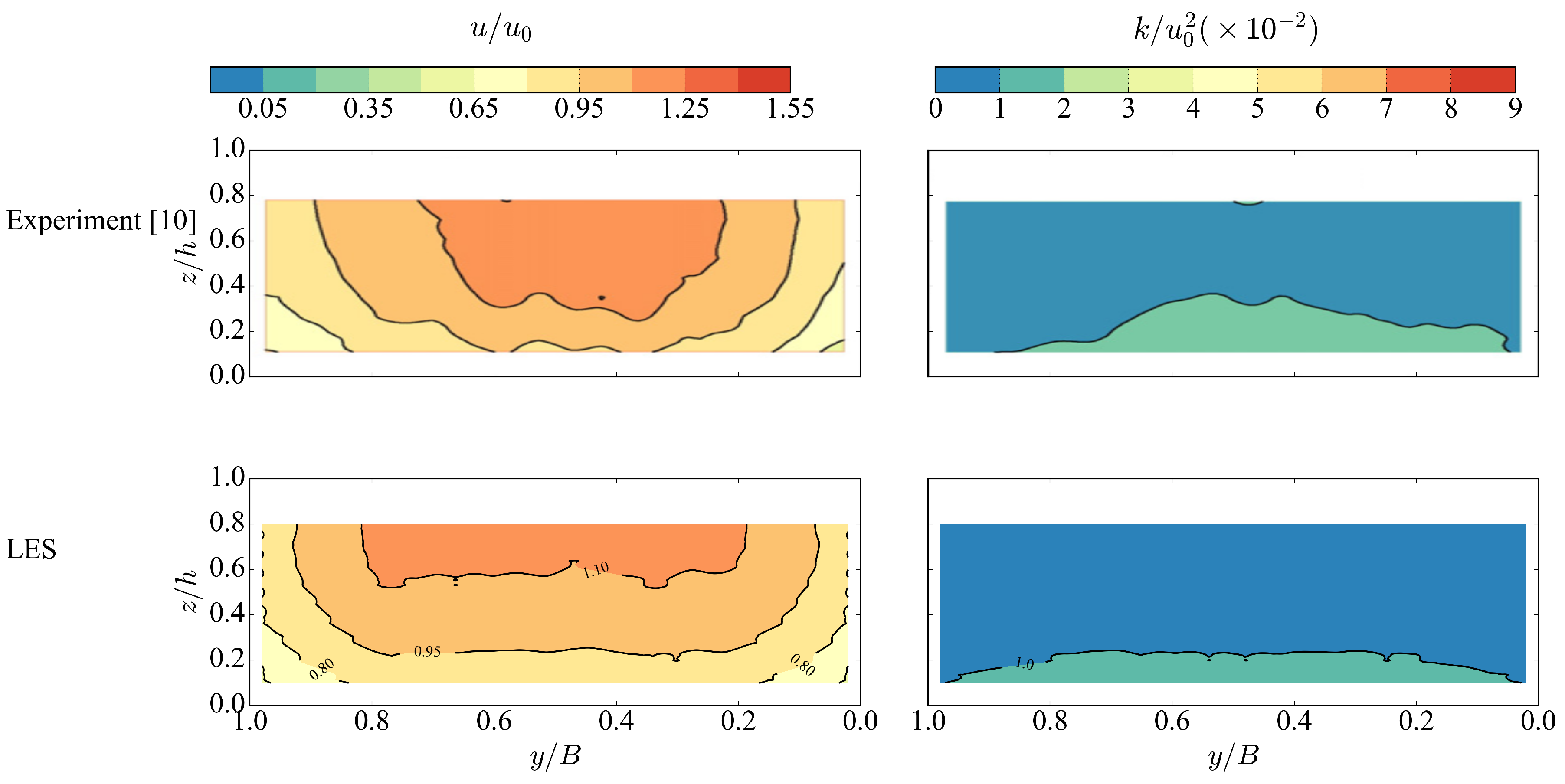
For the fully-resolved case, which serves as the baseline for the evaluation of the other two simplifications, we found that the turbulent inlet condition was critical for better comparison with the experiments in Bennett et al. [10]. In this study, a background case without ELJ was first run to get a fully-developed open channel flow, which was then used at the inlet. Figure 4 compares the cross-sectional distributions of mean streamwise velocity u and turbulent kinetic energy (TKE) k between the numerical and experimental results for the background case. The simulated mean fields were based on averages over 140 s, while in Bennett et al.’s [10] experiment, the averaging time was 180 s. The results from the 140 s averaging time have little difference from those with 100 s averaging time. Therefore, the 140 s averaging time was used in this work. From the comparison in the figure, a similar pattern and comparable magnitude can be observed for both velocity and TKE. The velocity core is slightly stretched in the simulation than in the experiment.

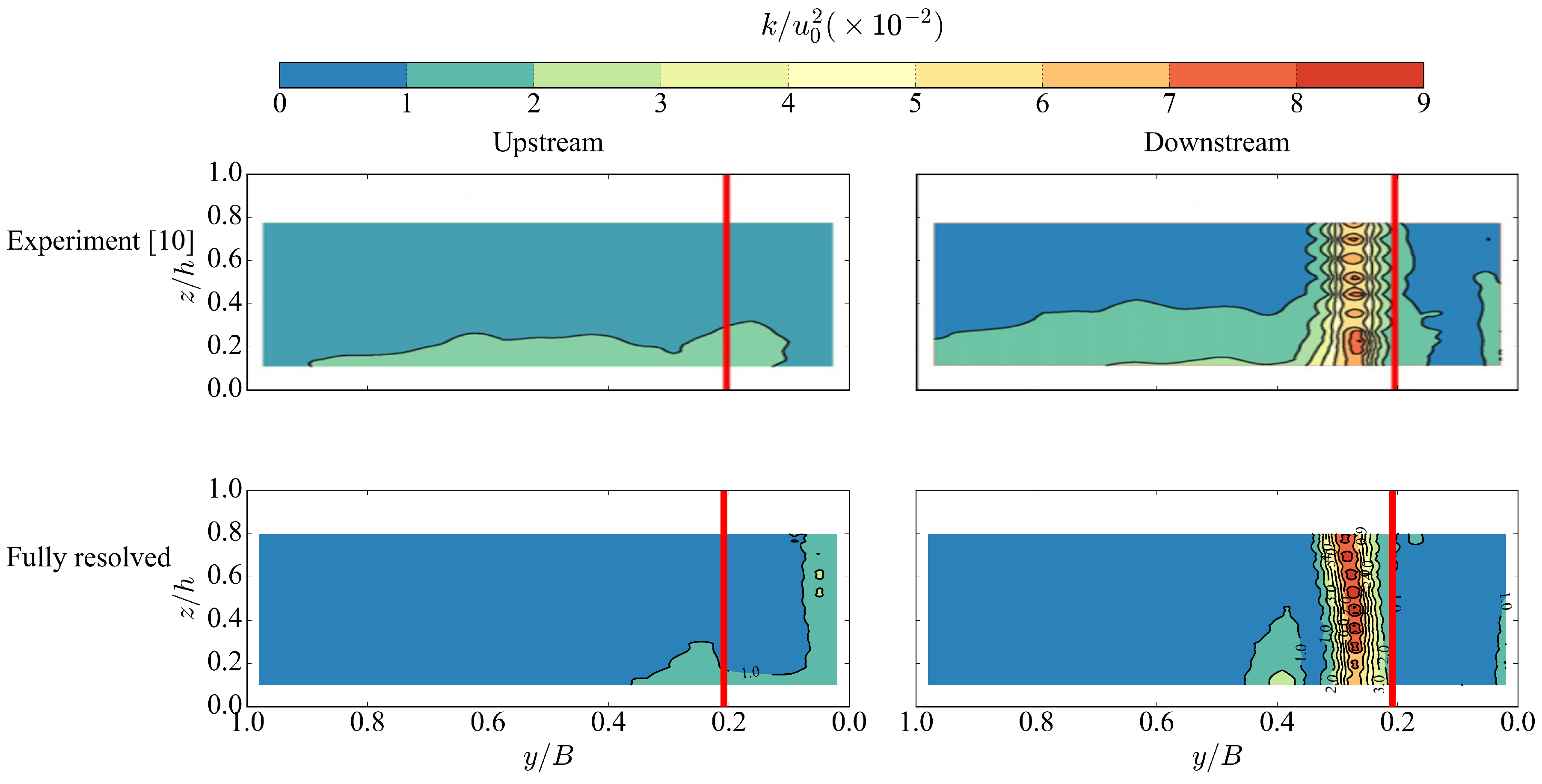
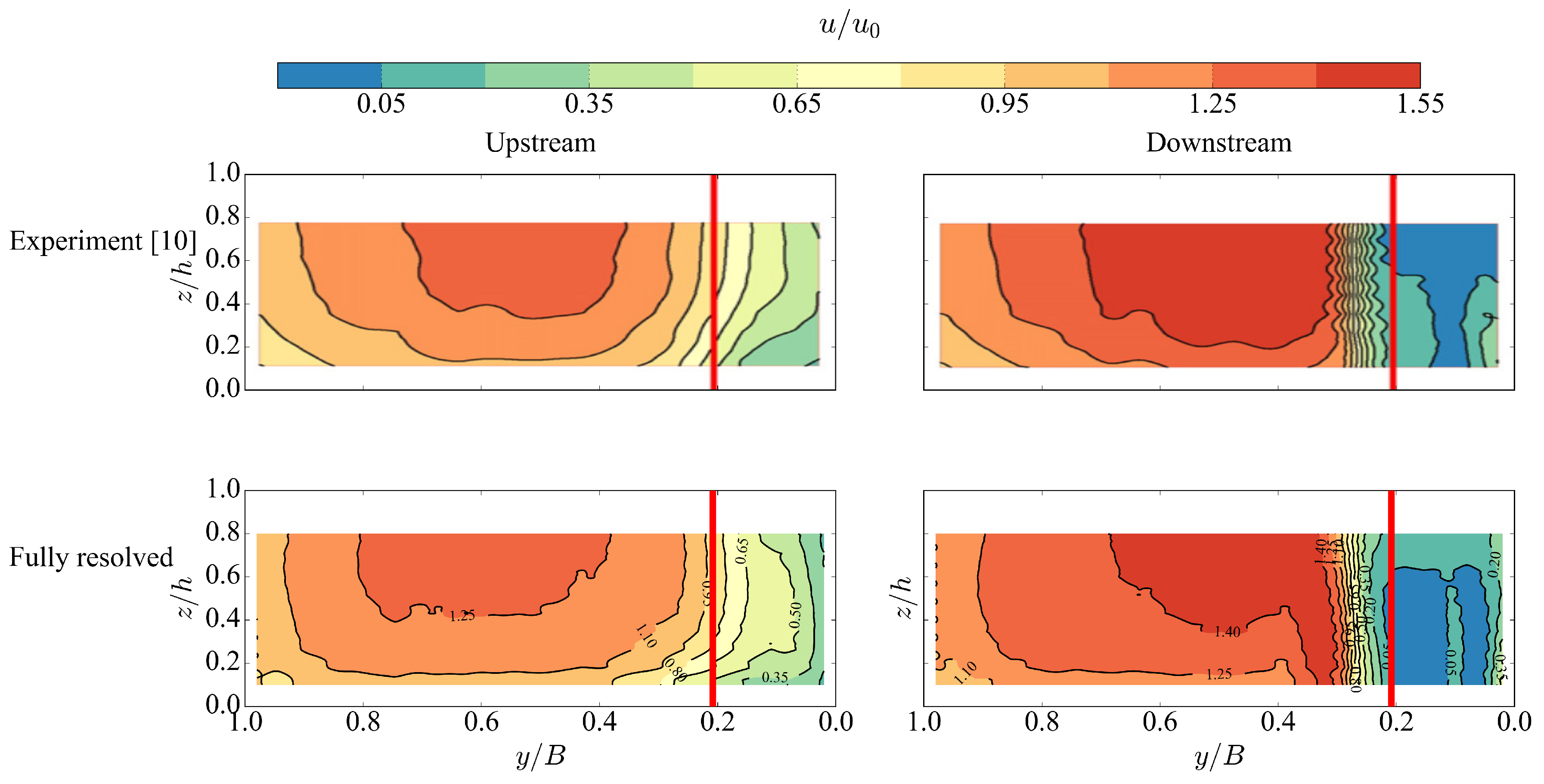
Bennett et al. [10] measured the flow on two cross-sections located at the immediate upstream and downstream sides of ELJ at $x=-95$ mm and $x=545$ mm, respectively. Figure 5 presents the comparison of the upstream and downstream cross-sectional distribution of the mean streamwise velocity. ELJ was located adjacent to the right sidewall (looking downstream). The red lines indicate the edge of ELJ. On the upstream cross-section, reduced velocity can be observed in the front of ELJ. The pattern and magnitude are quite similar in both experiment and the simulation. However, the high flow region from computational model slightly deviates from the experiment, which might be due to the flattened high velocity core in the simulated incoming flow. For the downstream cross-section, a large velocity gradient can be observed on the eddy of ELJ in both cases. The velocity in the upper main channel flow adjacent to ELJ is slightly larger in LES than in the experiment. However, they are very comparable in general.

The fully-resolved simulation case also shows good overall agreement on TKE with the experiment (Figure 6). In the computational model, the TKE k was calculated as:

$$k=k^{SGS}+{\displaystyle \frac{1}{2}}\left(u_x^{\prime 2}+u_y^{\prime 2}+u_z^{\prime 2}\right)$$

(16)

where $u^{\prime }$ denotes the resolved velocity fluctuation in three directions and $k^{SGS}$ denotes the unresolved sub-grid scale kinetic energy. The simulated upstream distribution of TKE has a noticeable difference from the experiment because of the overall small magnitude. For the downstream cross-section, the shear layer induced by ELJ created a high TKE zone, which was captured well by the computational model.

In the fully-resolved case, the drag force on ELJ can be directly calculated with the integration of pressure and shear stress on the structure surface, namely the first method, which gives $F_d=0.592\pm 0.042N$. The second method of using the momentum equation with the simulated flow field gives $F_d=0.596N$, which is very close to the result from the first method. For comparison, the measured drag force in Bennett et al. [10] was $F_d=0.851\pm 0.060N$, which indicates that the simulation underestimated the drag force. This underestimation might be attributed to several factors, including the incoming flow condition, the mismatch between the fabricated ELJ in experiment and the design, etc. In particular, the incoming flow cannot be exactly reproduced as seen in Figure 4, which leads to slower impingement onto ELJ and lower drag force. In the experiment, it will be ideal, but very time consuming, to measure in great detail the inflow conditions to be used at the inlet in the simulations. In this way, the discrepancy could be greatly reduced.

From the above comparison on mean velocity, TKE and drag force, the fully-resolved case reproduced the experimental condition well considering the complexity of the problem. In the following, the fully-resolved case will be used as the base for comparison with the porous media and solid barrier simplifications.

3.2. Calibration of Porous Media Model

The calibration of the porous media parameters (α, β and $d_{50}$) is based on the fully-resolved case, which itself has been validated with experiments in previous section. As summarized in Burcharth et al. [37] and Jensen et al. [29], the selection of α and β varies for different porous materials and packing modes. Six combinations of α, β and $d_{50}$ were tested for the ELJ structure. Table 1 lists the parameters, including the intrinsic and inertial permeability, of the six different combinations.

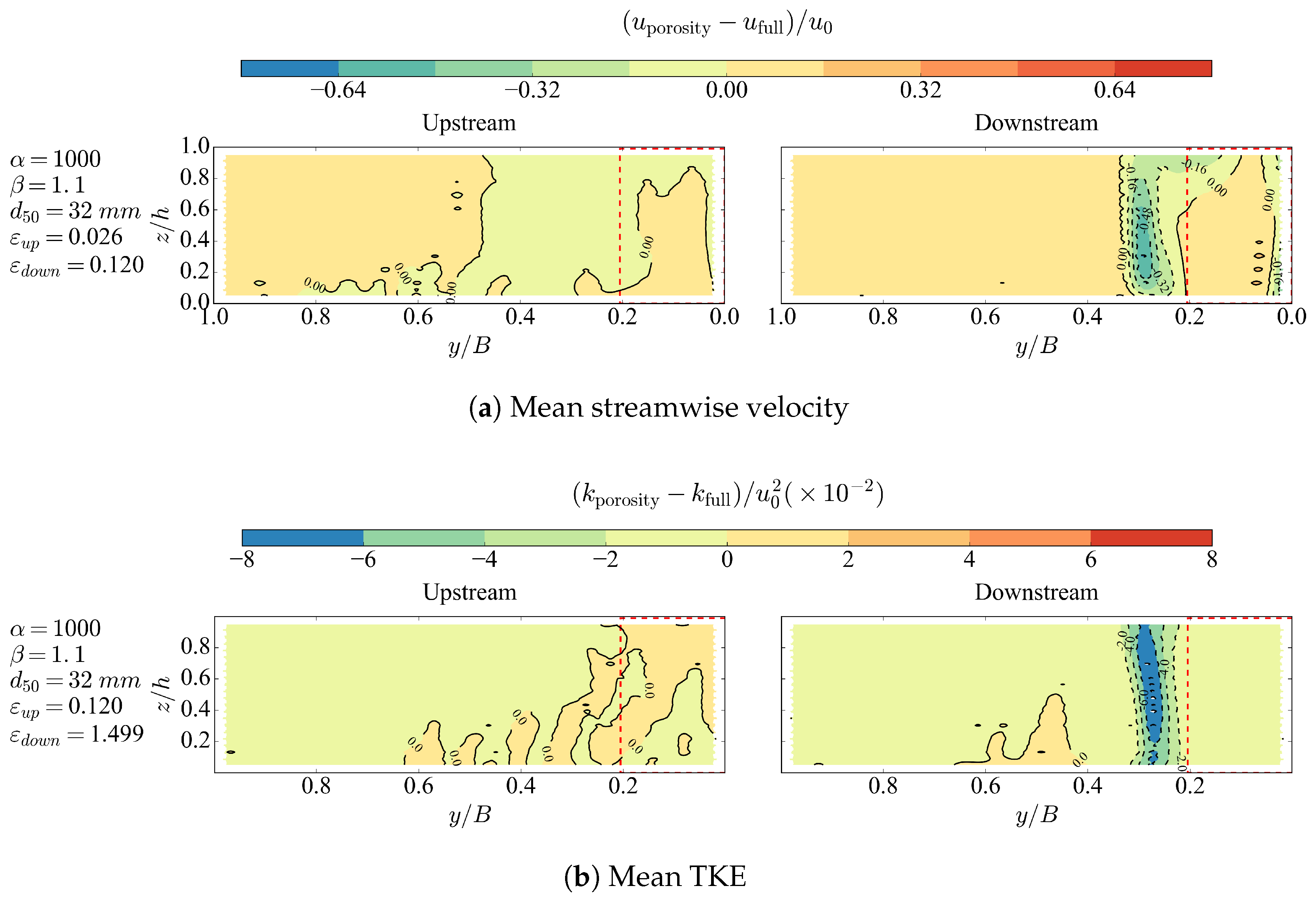
To quantify the difference between the porosity cases and the fully-resolved case, the cross-sectional error distributions for mean velocity and mean TKE are plotted in Figure 7. The error is defined as the porous media model results minus the fully-resolved simulation values. Figure 8 shows the transverse distribution of mean streamwise velocity and TKE on the upstream and downstream cross-sections at $z/z_0=0.4$. To reduce the length of this paper, we only plot the results from the case of $\alpha =1000$ and $\beta =1.1$, which gives better results than the case of $\alpha =200$ and $\beta =2$. The red dashed rectangle represents the location of ELJ. As shown in Figure 7a and Figure 8, for the upstream cross-section, large velocity errors mainly occur near the bed for small $d_{50}$. When $d_{50}$ is small (1 mm), the porosity model underestimates the streamwise velocity at the upstream side of ELJ, which is caused by the lower permeability suppressing the flow. The velocity suppression is more significant near the bank and free surface. In contrast, larger $d_{50}$ leads to higher permeability and thus overestimates the streamwise velocity in the upstream side of ELJ. For the downstream cross-sections, error occurs mainly in the shear layer. All porosity model cases underestimate the streamwise velocity in the shear layer, with slight overestimation in the near bed region. This near-bed overestimation is less significant when $d_{50}$ has the value of the key element diameter. For the TKE distribution shown in Figure 7b and Figure 8, the error distribution is different from velocity. With $d_{50}=$ 32 mm and 19 mm, TKE was under-predicted in the shear layer. However, if $d_{50}$ is very small (1 mm), TKE was dramatically over-predicted in the shear layer. This is caused by the fact that lower permeability of the porous media region forces more flow to the main channel and generates a larger velocity gradient in the shear layer.

In addition to the overall difference of velocity and TKE, an integral error over a cross-sectional plane can be defined as:

$$\epsilon ={\displaystyle \frac{1}{A_{\mathrm{Surf}}}}\sum _{i=0}^N\left[{\left({\eta }_{\mathrm{porosity},i}-{\eta }_{\mathrm{full},i}\right)}^2\Delta A_i\right]$$

(17)

where $A_{\mathrm{Surf}}$ denotes the total area of the surface, $\Delta A_i$ denotes the area for the i-th sub-area and ${\eta }_i$ denotes the flow variable on the i-th sub-area. As shown in Table 1, the general trend is that smaller $d_{50}$ resulted in smaller permeability, and the error ε became larger for both upstream and downstream velocity and TKE. However, the drag force error does not always follow this trend. For all six calibration cases, the results also show that the downstream error ε is always larger than the upstream due to the rich turbulent dynamics behind the ELJ. As seen in Table 1, the solid barrier case also over-predicted the drag force, and the error is much larger than that of the porosity case. The solid barrier case is closer to the $d_{50}=$ 1 mm porosity case in terms of drag force and spacial integral error.

Overall, based on the results for drag force $F_d$ and error ε, the combination of $\alpha =1000$, $\beta =1.1$ and $d_{50}=32$ mm gave the best results and, thus, was selected for further analysis.

3.3. Evaluation of Different Representations in the CFD Model

The effects of ELJ representation were investigated with three cases, including the validated fully-resolved case, the calibrated porous media case and the solid barrier case. The aspects of the ELJ hydraulics evaluated included flow adjustment, near-surface and near-bottom flow and turbulence and flow structure.

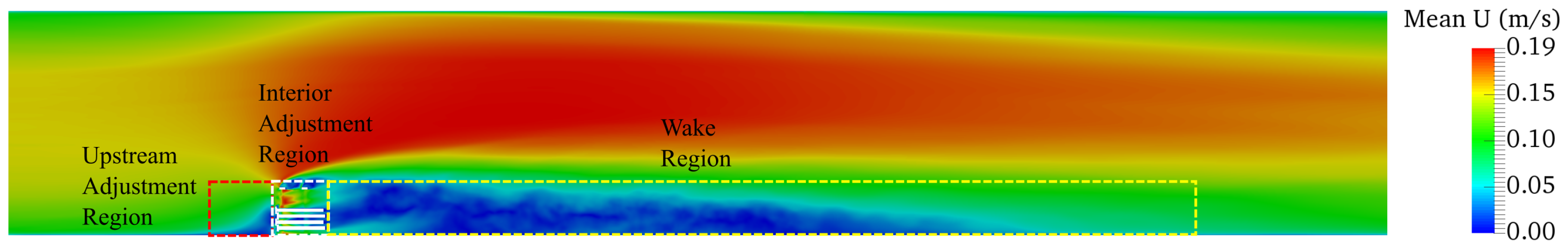
3.3.1. Flow Adjustment

To the best of our knowledge, there is no quantitative study on how flow will adjust when it passes an in-stream structure, which is usually bounded by stream banks. However, some recent studies investigated unbounded flow around finite and semi-finite (porous) vegetation patches [38,39,40]. They revealed the relationship between the porous media properties and the flow adjustment in terms of streamwise velocity and wake length. We used similar analysis with the aim to find comparable relationships. 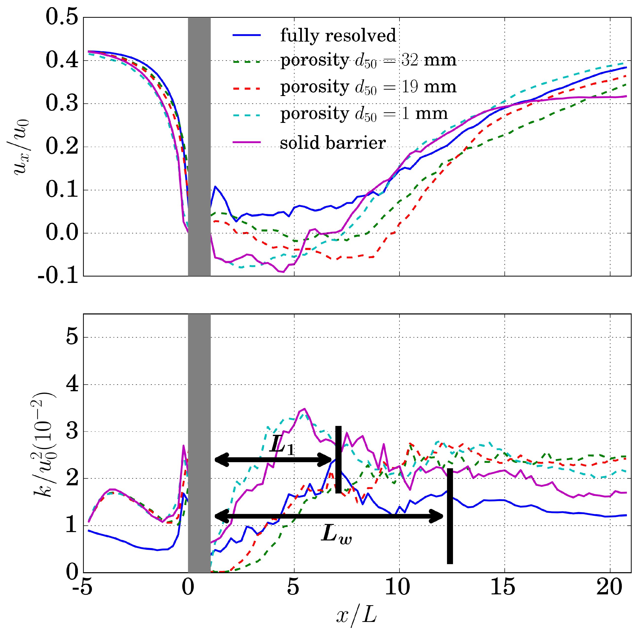As in previous studies [39,40], the flow domain can be partitioned into three regions as shown in Figure 9, namely the upstream adjustment region, the interior adjustment region and the wake region. For unbounded wake flows, two wake length scales ($L_1$ and $L_w$) can be defined. $L_1$ denotes the length scale of the steady wake region where the velocity remains almost constant. $L_w$ denotes the length scale of the distance between the structure and the von Karmen vortex street. However, Kim et al. [41] showed that the von Karmen vortex street cannot form in semi-bounded flows, which is consistent with the numerical results in this paper. These two lengths also manifest themselves in the signature of turbulence. $L_1$ is approximately located at the first peak of turbulence intensity in the wake region, while $L_w$ is located at the second peak. Chen et al. [40] proposed the following empirical wake length equations:

$${\displaystyle \frac{L_1}{L}}=\left\{\begin{array}{cc}2.5\left[{\displaystyle \frac{8-C_{d}aW}{C_{d}aW}}\right]\hfill & \mathrm{if}{C}_{d}aW<4\hfill \\ 2.5\hfill & \mathrm{if}{C}_{d}aW>4\hfill \end{array}\right.$$

(18)

$${\displaystyle \frac{L_w}{L}}=\left\{\begin{array}{cc}1.2\hfill & \mathrm{if}{C}_{d}aW>20\hfill \\ 1.2+(25\pm 10)C_{d}a{W}^{-0.9\pm 0.2}\hfill & \mathrm{if}{C}_{d}aW<20\hfill \end{array}\right.$$

(19)

where $C_d$ can be calculated with Equation (13). $a=md$, where m is the element number per unit planar area and d is the diameter of the cylindrical element used in Chen et al. [40]. $C_{d}aW$ denotes the flow blockage due to the obstruction. For ELJ, we use the key elements to approximate n and d. As a result, $d=0.032$m and $m=14/(0.4$m$\times 0.5$m).

Chen et al. [40] measured the centerline velocity at half depth in flume experiments to represent the depth-averaged velocity for their unbounded flow around a porous vegetation patch. In this study, since we have the simulated velocity distribution around ELJ, local cross-sectional averaging was performed within the adjustment and wake regions. Local regional averaging is more suitable for this semi-bounded flow. Figure 10 shows the longitudinal profiles of cross-sectionally-averaged streamwise velocity and TKE within the adjustment and wake regions. For the velocity profile, due to the semi-boundedness (wall effect), the incoming normalized streamwise velocity is only about 0.43. The trend of the velocity profiles is in accordance with that in Chen et al. [40]. 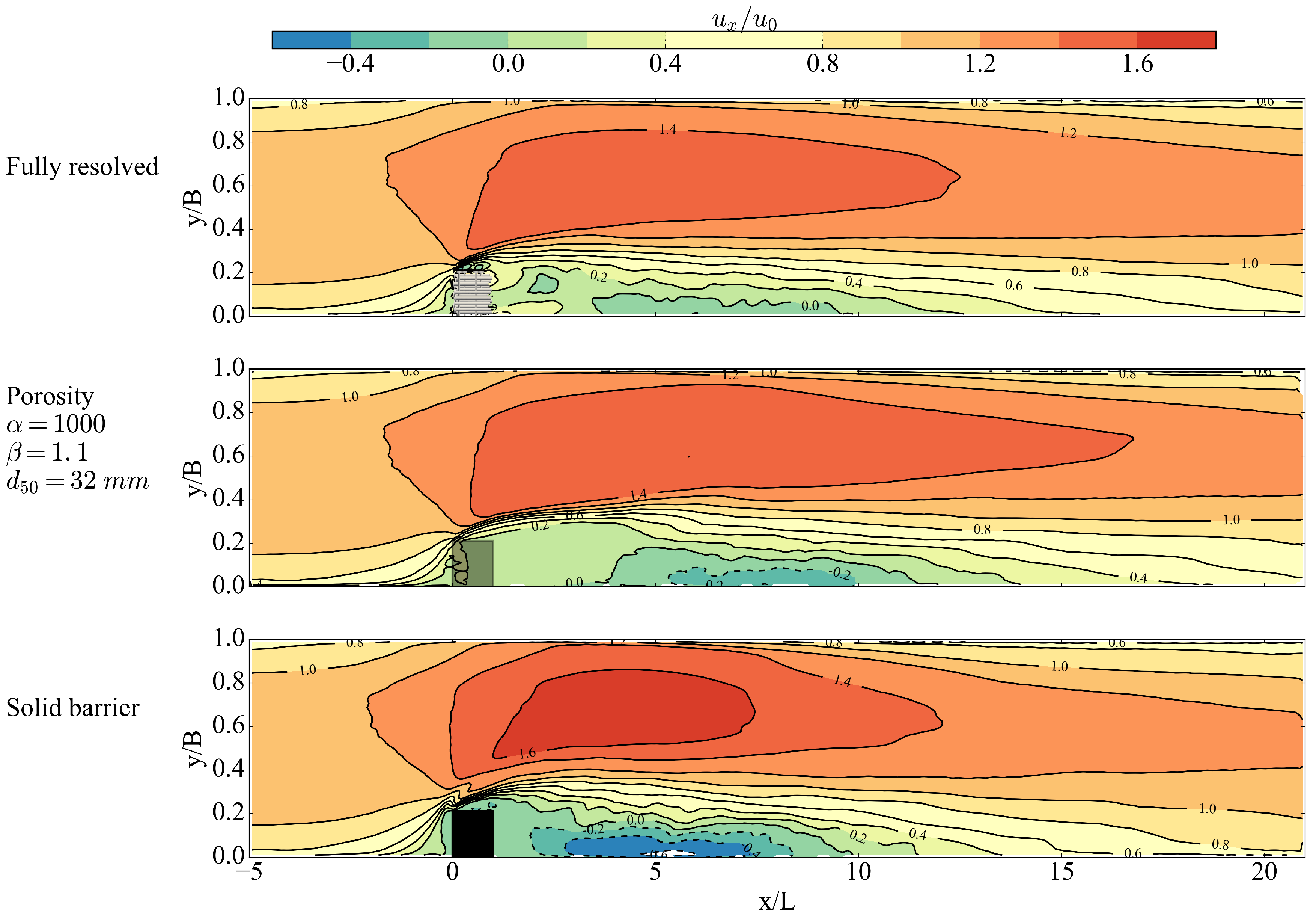In the steady wake region, the larger pore size ($d_{50}$) case tends to match better with the fully-resolved case. The velocity profiles of solid barrier and small pore size case are similar, which makes sense because the small pore size reduces the permeability. They both show negative streamwise velocity inside the steady wake region. This is induced by the strong boundary layer separation and vortex generated at the edge of the object. With the increase of porosity, more passing-through flow reduces the negative pressure gradient, pushes the wake flow further downstream and thus enlarges the wake. For TKE, it has a relatively large value at the upstream side of ELJ edge and a small value at the immediate downstream side where the area is shielded. After that, TKE increases rapidly in the steady wake region. We also found that the growth rate and asymptotic TKE value are affected by the permeability and the resulted flow passing through ELJ. Reduced pass-through flow will induce higher shear, more eddies and, thus, higher TKE in the steady wake region. Neither the porosity model cases, nor the solid barrier case reproduced a good match on TKE in the whole of the wake zones. The porosity model with a large pore size matched with the fully-resolved case in the steady wake zone, while the solid barrier case matched better further downstream. For all porosity model cases, they tend to maintain high turbulence even after the steady wake region.

Table 2. Measured wake length $L_1$ and $L_w$.

	${\mathit{L}}_1$	${\mathit{L}}_{\mathit{w}}$
Fully resolved	6.1	11.3
Porosity $d_{50}=32$ mm	7.8	$10\sim 13$
Porosity $d_{50}=19$ mm	6.3	$10\sim 13$
Porosity $d_{50}=1$ mm	4.6	$10\sim 13$
Solid barrier	4.5	7.6

shows the simulated $L_1$ and $L_w$ from the cases shown in Figure 10. The length scales were determined by the peak of turbulent intensity. However, we found that for the porosity cases, it was very difficult to determine the exact value of $L_w$ due to the lack of clear peaks, as shown in Figure 10. Thus, only the range of $L_w$ is presented. The results indicate that the porosity model with $d_{50}$ = 19 mm produced a better match on $L_1$ with the fully-resolved case. Again, the increase of $d_{50}$, i.e., porosity, will increase the wake length $L_1$. According to Equations (13), (18) and (19), if we use the channel mean velocity in the equations, we obtain $C_{d}aW=1.7$, $L_1=20.1L$ and $L_w=36.5L$, which are much larger than the values in Table 2. However, if the mean velocity of the whole channel was replaced by the local mean value experienced by the ELJ, i.e., $U=0.43u_0$, we obtain $C_{d}aW=9.4$, $L_1=5.6L$ and $L_w=10.1L$. Obviously, the latter is closer to the simulated values. The replacement of incoming flow velocity with the local mean is reasonable and necessary because of the side wall effects.

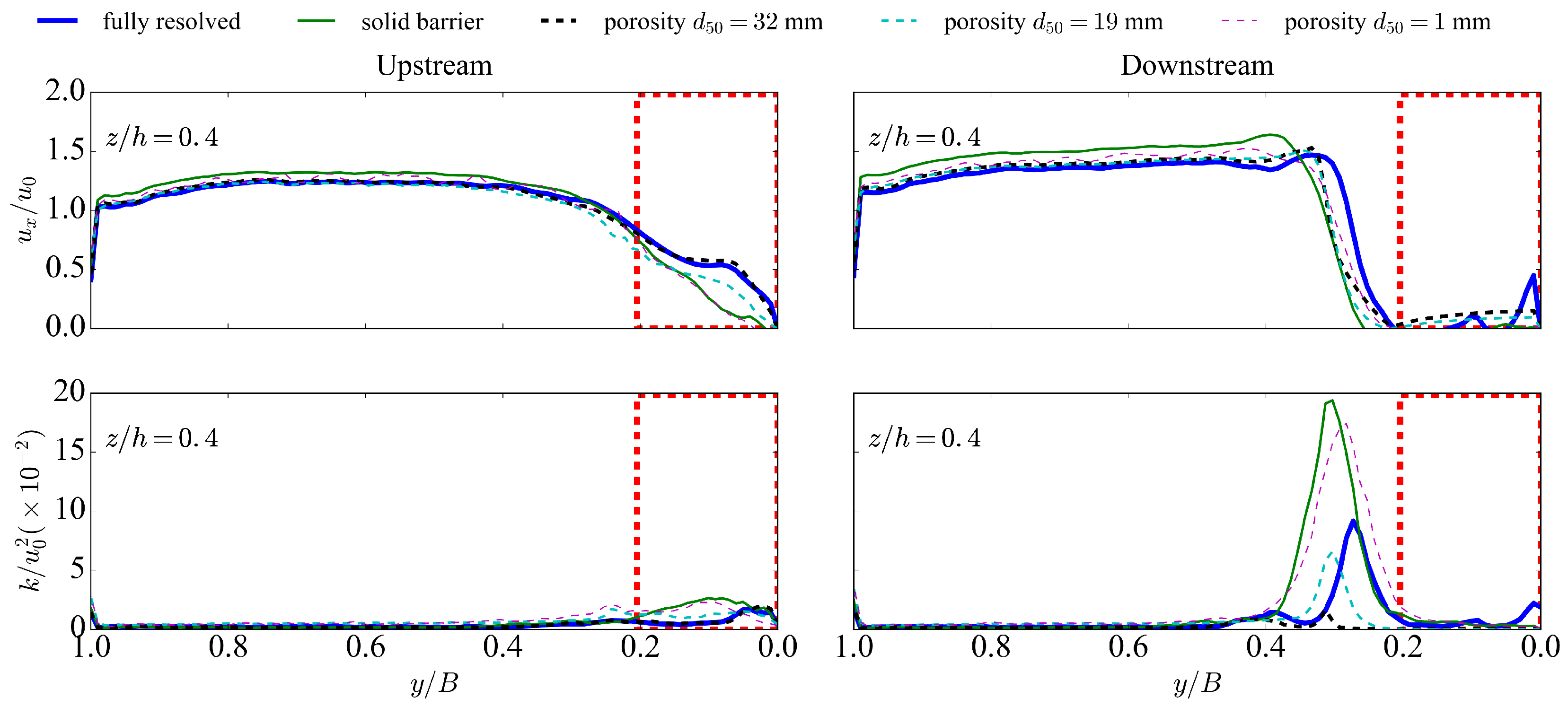
3.3.2. Near-Surface Velocity

Another important metric is the near-surface velocity around the in-stream structure, which impacts a host of processes, such as aeration and heat transfer. Figure 11 shows the time-averaged streamwise velocity distribution at 5 mm below the free surface for different cases. For the porosity model, only the case with $\alpha =1000$, $\beta =1.1$ and $d_{50}=32$ mm is shown. The comparison shows that the surface velocity is not so sensitive to how ELJ is modeled. The only noticeable difference is in the steady wake region. For the fully-resolved case and the porosity case, there is only a small region showing negative streamwise velocity. However, for the solid barrier case, a much larger region has negative streamwise velocity, which is due to the fact that no passing-through flow causes much stronger recirculation behind the solid barrier. This result is consistent with Figure 10.

3.3.3. Near-Bed Turbulence

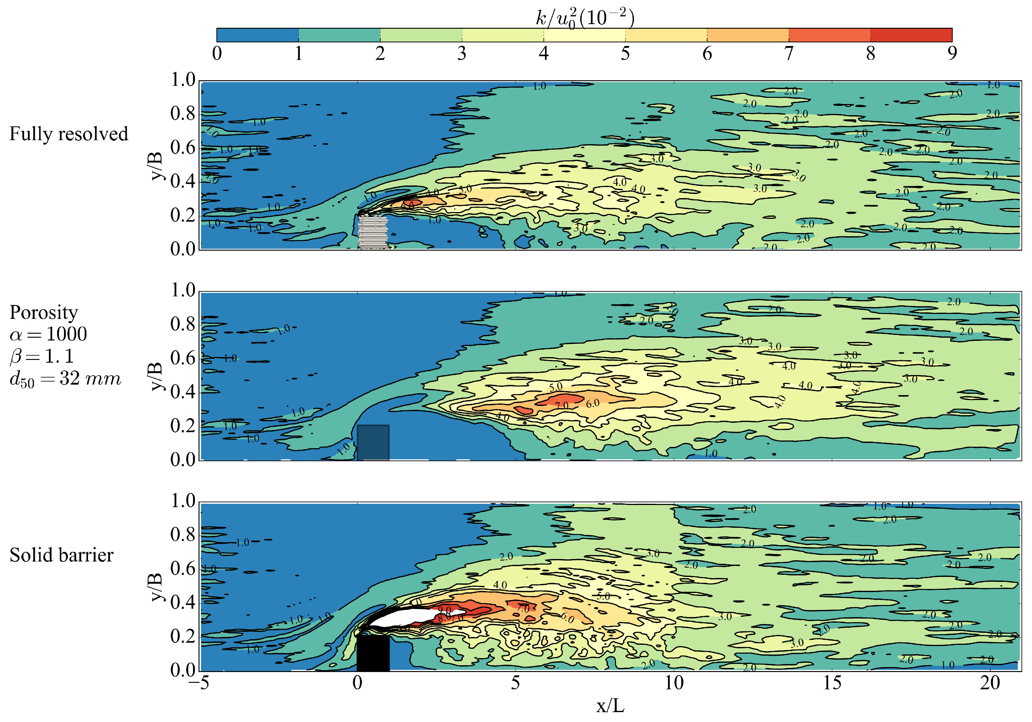
In-stream structures also affect river morphology by changing sediment transport. Thus, near-bed turbulence, the driver of sediment motion, is evaluated. The time-averaged TKE near the bed is used as a proxy for sediment entrainment capacity [42]. The near-bed TKE distributions are plotted in Figure 12. The data were sampled at a height of 15 mm above the bed. From the comparison, it is observed that the porosity model gave a better match with the fully-resolved case. The porosity model underestimated TKE in the shear layer, and the shear layer itself was delayed. The solid barrier case greatly overestimated TKE in the shear layer. Thus, from the sediment transport point of view, the solid barrier approximation to the ELJ will over-predict the scour hole around the structure.

3.3.4. Flow Structure

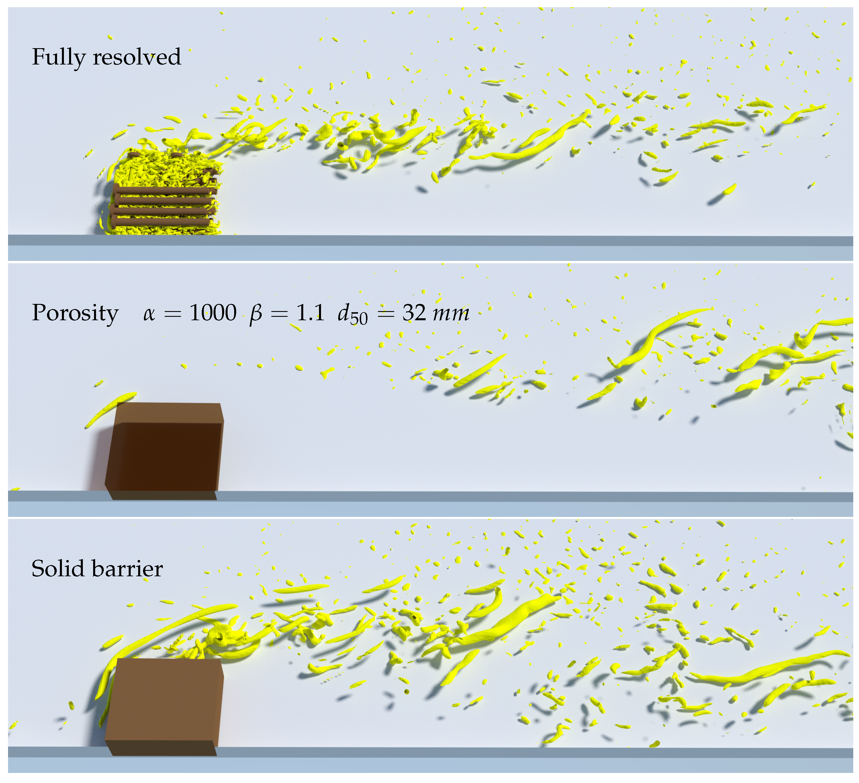
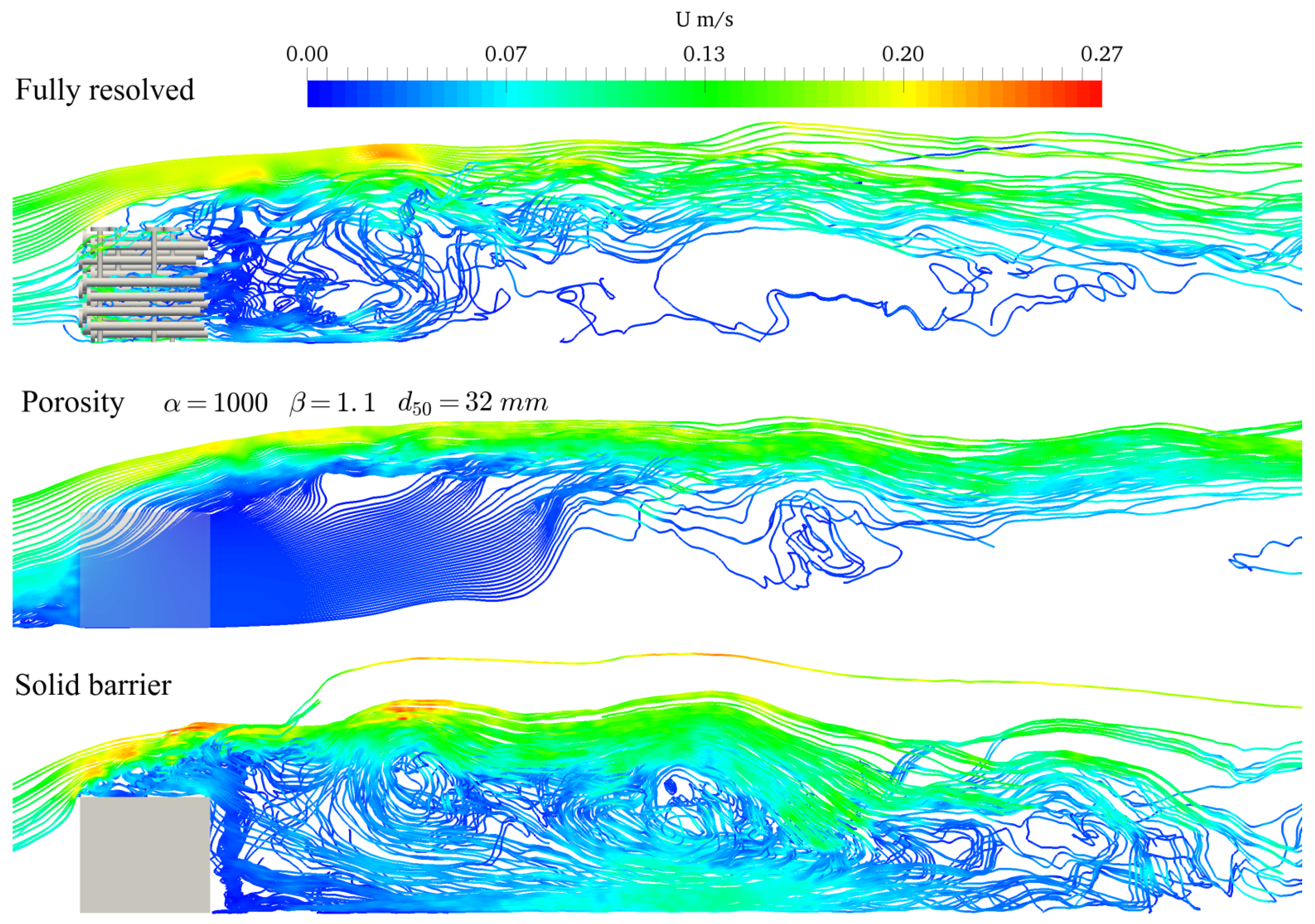
The effects of ELJ representation in models can be evaluated at the simulated flow features. Figure 13 shows an instantaneous flow field (streamlines) in the wake zone, which is colored by the magnitude of instantaneous velocity. These streamlines were sourced from a horizontal line parallel to the downstream side of ELJ. The source line was located at 50 mm above the bed. As can be seen in the figure, significant discrepancy exists in the steady wake zone in different model representations. For the fully-resolved case, small and irregular flow curvatures can be observed in the steady wake zone, most of which stem from the element surface in ELJ. The incoming flow has to go through the irregular pores within ELJ, and it results in very rich flow dynamics. In the porous media case, such dynamics are totally lost, and the streamlines are much smoother than the other two cases in the steady wake zone. Low permeability in the porous media region only slows down the flow through ELJ. The only similarity between the porous media case and the fully-resolved case is that the passing-through flow causes the delay of the shear layer. In the solid barrier case, a larger recirculation zone and a strong shear layer can be seen at the lee side of the block.

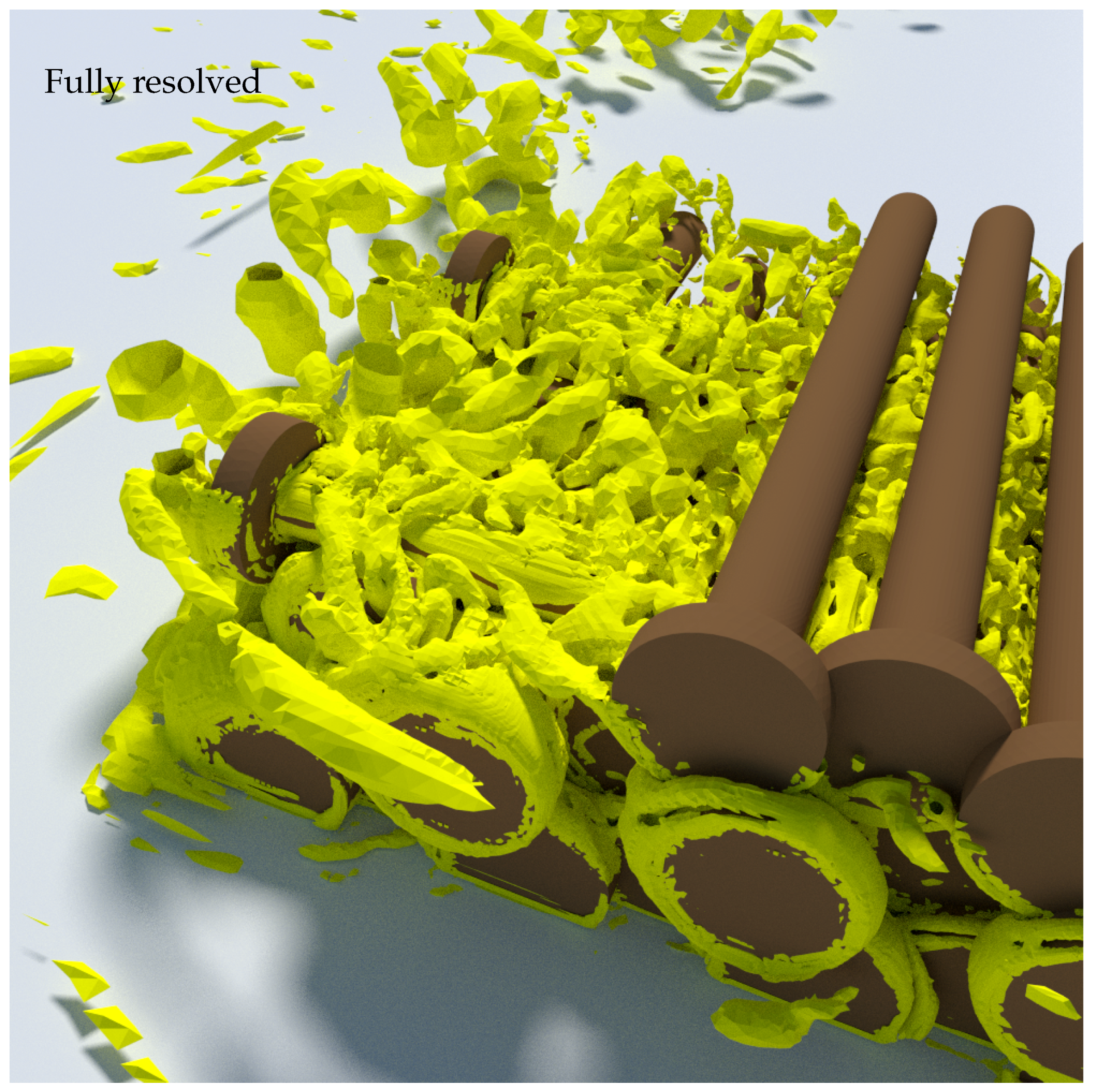
Figure 14 shows the instantaneous isosurfaces of ${\lambda }_2$ = 3. ${\lambda }_2$ is a commonly-used flow quantity to visualize the vortex structures [43]. Substantial differences can be observed among the three cases. The fully-resolved case shows strong coherent flow structures inside the ELJ, also shown in Figure 15. In the shear layer, it takes a long distance for the vortex to shed behind the ELJ to re-attach to the right bank. However, in the porous media case, no such coherent structure was observed inside the porous media domain at the same value of ${\lambda }_2$. The vortex structure is also extremely weak in the near-field compared with the fully-resolved case. However, it shows similar vortex structure in the far-field as the fully-resolved case. In the solid barrier case, the contour of ${\lambda }_2$ = 3 shows comparable strong coherent structures as the fully-resolved case in the near-field shear layer. However, the shear layer of the solid barrier case is more diffusive in the far field than the other two cases. In addition, the reattachment distance is much smaller in the solid barrier case. This reduction of reattachment distance is caused by the lack of passing-through flow in the solid barrier case. Overall, in terms of flow structure, the porous media case models well in the far field, while the solid barrier case predicts better in the near field. Nevertheless, neither of them are able to resolve the flow structure inside the ELJ.

4. Conclusions

Using three-dimensional computational fluid dynamics modeling, we evaluated the effects of different modeling representations of ELJ, a popular in-stream structure for river restoration and erosion control. Three different modeling cases, i.e., a fully-resolved case, a porosity model case and a solid barrier case, were simulated. The computational model was validated with experimental data in a flume where a scaled model of ELJ was placed. The simulated results were examined and analyzed on various aspects related to the functionality and stability of ELJ. The applicabilities and limitations of each simplified representation of complex ELJ geometry were discussed.

Full resolution of the ELJ geometry is not feasible for wide use in practice because of the prohibitive computational cost. In this work, it served as the baseline for comparison with other methods. The fully-resolved case reproduced the velocity and TKE distributions well at the upstream and downstream cross-sections near the ELJ. When the porosity model was used, the porosity coefficients were first calibrated to get $\alpha =1000$, $\beta =1.1$, $d_{50}=32$ mm. We found that the equivalent grain size $d_{50}$ should scale as the key element diameter in this particular ELJ. The calibrated porosity model only showed satisfactory performance on drag force, velocity and TKE. The solid barrier case generally gave the least accurate results.

Further comparison showed that the modeling of the passing-through flow has a significant impact on the wake and the shear layer, which is summarized in

Table 3. Comparison between the porosity model and the solid barrier model.

	Porosity	Solid Barrier
near-bed TKE	under-predicted	over-predicted
near-field flow structure	well-predicted	extremely weak
far-field flow structure	too diffusive	well predicted
flow structure inside ELJ	unpredictable	unpredictable
wake length $L_1$ and $L_w$	under-predicted	over-predicted
computational efforts (of fully resolved)	about 1/200	about 1/50
drag force (of fully resolved)	about 1.11	about 1.25

. The porosity model approximates the near-surface velocity and near-bed TKE in the steady wake region well, while the solid barrier model performed slightly better further downstream. According to the near-bed TKE, the shear layer is under-predicted in the porosity model and over-predicted in the solid barrier model. The solid barrier model can predict well the strong flow structure in the near-field shear layer, while the porosity model performs better in the far-field shear layer. However, neither the porosity model, nor the solid barrier model can capture the flow structure inside the ELJ. The flow adjustment analysis shows that patches with higher flow blockage ($C_{d}aW$) have larger wake length. The wake lengths $L_1$ and $L_w$ from Equations (18) and (19) agree well with simulated results only if the local velocity, instead of channel mean velocity, is used.

In conclusion, when the porosity model or solid barrier representation is used for ELJ, the benefits of the significantly reduced computational cost come with the price of missing physical information that might be important for the intended purpose of in-stream structures. The porosity model, after careful calibration, seems to perform better than the solid barrier model, especially the drag force. However, this work also identified substantial loss of accuracy in terms of velocity, turbulent shear, sediment transport capacity and coherent structure in the vicinity and the wake zone of ELJ. Thus, care needs to be taken to interpret and use the porosity model results in practice. If the emphasis is in the far field, then the simulation results using both the porosity model and the solid barrier representation did not show dramatic difference from the fully-resolved case. Therefore, the use of such simplified models may be justified.

References

1. Shields, F.D.; Nunnally, N.R. Environmental aspects of clearing and snagging. J. Environ. Eng. 1984, 110, 152–165. [Google Scholar] [CrossRef]
2. Bisson, P.; Bilby, R.; Bryant, M.; Dolloff, C. Large woody debris in forested streams in the Pacific Northwest: Past, present, and future. In Streamside Management: Forestry and Fishery Interactions; College of Forest Resources, University of Washington: Seattle, WA, USA, 1987; pp. 143–190. [Google Scholar]
3. Sullivan, K.; Lisle, T.E.; Dolloff, C.A.; Grant, G.E.; Reid, L.M. Stream channels: The link between forest and fishes. In Streamside Management: Forestry and Fishery Interactions, Proceedings of a Symposium Held at University of Washington; Salo, E.O., Cundy, T.W., Eds.; University of Washington: Seattle, WA, USA, 1987; Chapter 3; pp. 39–97. [Google Scholar]
4. Gorman, O.T.; Karr, J.R. Habitat structure and stream fish communities. Ecology 1978, 59, 507–515. [Google Scholar] [CrossRef]
5. Bilby, R.E.; Likens, G.E. Importance of organic debris dams in the structure and function of stream ecosystems. Ecology 1980, 61, 1107–1113. [Google Scholar] [CrossRef]
6. Tullos, D.; Walter, C. Fish use of turbulence around wood in winter: Physical experiments on hydraulic variability and habitat selection by juvenile coho salmon, Oncorhynchus kisutch. Environ. Biol. Fish. 2015, 98, 1339–1353. [Google Scholar] [CrossRef]
7. Fausch, K.D. Profitable stream positions for salmonids: Relating specific growth rate to net energy gain. Can. J. Zool. 1984, 62, 441–451. [Google Scholar] [CrossRef]
8. Bernhardt, E.S.; Palmer, M.A.; Allan, J.D.; Alexander, G.; Barnas, K.; Brooks, S.; Carr, J.; Clayton, S.; Dahm, C.; Galat, D.; et al. Synthesizing U.S. river restoration efforts. Science 2005, 308, 636–637. [Google Scholar] [CrossRef] [PubMed]
9. Jarrett, A.R.; Brannaka, L.K.; Ballestero, T. Elements of Stream Restoration, 2nd ed.; Stream Restoration Workshops: University Park, PA, USA, 2011. [Google Scholar]
10. Bennett, S.J.; Ghaneeizad, S.M.; Gallisdorfer, M.S.; Cai, D.; Atkinson, J.F.; Simon, A.; Langendoen, E.J. Flow, turbulence, and drag associated with engineered log jams in a fixed-bed experimental channel. Geomorphology 2015, 248, 172–184. [Google Scholar] [CrossRef]
11. Gippel, C.J. Environmental hydraulics of large woody debris in streams and rivers. J. Environ. Eng. 1995, 121, 388–395. [Google Scholar] [CrossRef]
12. Manga, M.; Kirchner, J.W. Stress partitioning in streams by large woody debris. Water Resour. Res. 2000, 36, 2373. [Google Scholar] [CrossRef]
13. Wenzel, R.; Reinhardt-Imjela, C.; Schulte, A.; Bölscher, J. The potential of in-channel large woody debris in transforming discharge hydrographs in headwater areas (Ore Mountains, Southeastern Germany). Ecol. Eng. 2014, 71, 1–9. [Google Scholar] [CrossRef]
14. Einstein, H.A.; Banks, R.B. Fluid resistance of composite roughness. Trans. Am. Geophys. Union 1950, 31, 603–610. [Google Scholar] [CrossRef]
15. Shields, F.D.; Gippel, C.J. Prediction of effects of woody debris removal on flow resistance. J. Hydraul. Eng. 1995, 121, 341–354. [Google Scholar] [CrossRef]
16. Wilcox, A.C.; Nelson, J.M.; Wohl, E.E. Flow resistance dynamics in step-pool channels: 2. Partitioning between grain, spill, and woody debris resistance. Water Resour. Res. 2006, 42, W05419. [Google Scholar] [CrossRef]
17. Young, W.J. Flume study of the hydraulic effects of large woody debris in lowland rivers. Regul. Rivers Res. Manag. 1991, 6, 203–211. [Google Scholar] [CrossRef]
18. Gippel, C.J.; O’Neill, I.C.; Finlayson, B. The Hydraulic Basis of Snag Management; Centre for Environmental Applied Hydrology, Department of Civil and Agricultural Engineering, University of Melbourne: Melbourne, Australia, 1992; p. 116. [Google Scholar]
19. Gippel, C.J.; O’Neill, I.C.; Finlayson, B.L.; Schnatz, I. Hydraulic guidelines for the re-introduction and management of large woody debris in lowland rivers. Regul. Rivers Res. Manag. 1996, 12, 223–236. [Google Scholar] [CrossRef]
20. Turcotte, B.; Millar, R.G.; Hassan, M.A. Drag forces on large cylinders. River Res. Appl. 2015, 32, 411–417. [Google Scholar] [CrossRef]
21. Manners, R.B.; Doyle, M.W.; Small, M.J. Structure and hydraulics of natural woody debris jams. Water Resour. Res. 2007, 43, W06432. [Google Scholar] [CrossRef]
22. Manners, R.B.; Doyle, M.W. A mechanistic model of woody debris jam evolution and its application to wood-based restoration and management. River Res. Appl. 2008, 24, 1104–1123. [Google Scholar] [CrossRef]
23. Shields, F.D.; Alonso, C.V. Assessment of flow forces on large wood in rivers. Water Resour. Res. 2012, 48, 1–16. [Google Scholar] [CrossRef]
24. Constantinescu, G.; Sukhodolov, A.; McCoy, A. Mass exchange in a shallow channel flow with a series of groynes: Les study and comparison with laboratory and field experiments. Environ. Fluid Mech. 2009, 9, 587–615. [Google Scholar] [CrossRef]
25. McCoy, A.; Constantinescu, G.; Weber, L. A numerical investigation of coherent structures and mass exchange processes in channel flow with two lateral submerged groynes. Water Resour. Res. 2007, 43, 1–26. [Google Scholar] [CrossRef]
26. Allen, J.B.; Smith, D.L. Characterizing the impact of geometric simplification on large woody debris using CFD. Int. J. Hydraul. Eng. 2012, 1, 1–14. [Google Scholar]
27. Gent, M.V. Wave Interaction with Permeable Coastal Structures; Technical Report Diss 2689; Delft University of Technology: Delft, The Netherlands, 1995. [Google Scholar]
28. Jensen, B. Wave Interaction with Porous Coastal Structures. Ph.D. Thesis, Technical University of Denmark, Kongens Lyngby, Denmark, 2014. [Google Scholar]
29. Jensen, B.; Jacobsen, N.G.G.; Christensen, E.D. Investigations on the porous media equations and resistance coefficients for coastal structures. Coast. Eng. 2014, 84, 56–72. [Google Scholar] [CrossRef]
30. Gallisdorfer, M.S.; Bennett, S.J.; Atkinson, J.F.; Ghaneeizad, S.M.; Brooks, A.P.; Simon, A.; Langendoen, E.J. Physical-scale model designs for engineered log jams in rivers. J. Hydro-Environ. Res. 2013, 8, 115–128. [Google Scholar] [CrossRef]
31. Smagorinsky, J. General circulation experiments with the primitive equations. Mon. Weather Rev. 1963, 91, 99–164. [Google Scholar] [CrossRef]
32. Deardorff, J.W. A numerical study of three-dimensional turbulent channel flow at large Reynolds numbers. J. Fluid Mech. 1970, 41, 453. [Google Scholar] [CrossRef]
33. Lilly, D.K. A proposed modification of the Germano-Subgrid-Scale closure method. Phys. Fluids 1992, 4, 633–635. [Google Scholar] [CrossRef]
34. Germano, M.; Piomelli, U.; Moin, P.; Cabot, W.H. A dynamic subgrid-scale eddy viscosity model. Phys. Fluids A Fluid Dyn. 1991, 3, 1760. [Google Scholar] [CrossRef]
35. OpenCFD. OpenFOAM: The Open Source Computational Fluid Dynamics (CFD) Toolbox. Available online: http://www.OpenFoam.org (accessed on 15 September 2016).
36. Spalding, D.B. A single formula for the “Law of the Wall”. J. Appl. Mech. 1961, 28, 455. [Google Scholar] [CrossRef]
37. Burcharth, H.; Anderson, O. On the one-dimensional steady and unsteady porous flow equations. Coast. Eng. 1995, 24, 233–257. [Google Scholar] [CrossRef]
38. White, B.L.; Nepf, H.M. Scalar transport in random cylinder arrays at moderate Reynolds number. J. Fluid Mech. 2003, 487, 43–79. [Google Scholar] [CrossRef]
39. Rominger, J.T.; Nepf, H.M. Flow adjustment and interior flow associated with a rectangular porous obstruction. J. Fluid Mech. 2011, 680, 636–659. [Google Scholar] [CrossRef]
40. Chen, Z.; Ortiz, A.; Zong, L.; Nepf, H. The wake structure behind a porous obstruction and its implications for deposition near a finite patch of emergent vegetation. Water Resour. Res. 2012, 48, 1–12. [Google Scholar] [CrossRef]
41. Kim, H.S.; Kimura, I.; Shimizu, Y. Bed morphological changes around a finite patch of vegetation. Earth Surf. Process. Landf. 2015, 40, 375–388. [Google Scholar] [CrossRef]
42. Yang, J.; Chung, H.; Nepf, H. The onset of sediment transport in vegetated channels predicted by turbulent kinetic energy. Geophys. Res. Lett. 2016, 43. [Google Scholar] [CrossRef]
43. Jeong, B.J.; Hussaini, M. On the identification of a vortex. J. Fluid Mech. 1995, 285, 69–94. [Google Scholar] [CrossRef]
Figure 1. The engineered log jam (ELJ) structure in the flume. In the 3D view, a fake free surface was added.
Water 09 00110 g001
Figure 2. Time averaged y+ distribution for the fully-resolved ELJ and the solid barrier.
Water 09 00110 g002
Figure 3. Zoom-in view of the fully-resolved ELJ mesh generated by snappyHexMesh.
Water 09 00110 g003
Figure 4. Comparison of the cross-sectional distributions of mean streamwise velocity and turbulent kinetic energy (TKE) between the numerical and experimental results for the background case without ELJ. The variables are made dimensionless with channel width B, water depth h and mean velocity u 0 .
Water 09 00110 g004
Figure 5. Comparison of the cross-sectional distributions of the mean streamwise velocity between the experiment and the fully-resolved case with ELJ.
Water 09 00110 g005
Figure 6. Comparison of the cross-sectional distributions of TKE between the experiment and the fully-resolved case with ELJ.
Water 09 00110 g006
Figure 7. Error distribution on the upstream and downstream cross-sections between the porosity cases and the fully-resolved case. The white blank region means that the values exceed the range of the colorbar.
Water 09 00110 g007
Figure 8. Transverse distribution of the mean streamwise velocity and TKE on the upstream and downstream cross-sections at z / h = 0.4 .
Water 09 00110 g008
Figure 9. Flow domain partition, colored by time-averaged velocity on the water surface.
Water 09 00110 g009
Figure 10. Longitudinal profiles of cross-sectionally-averaged streamwise velocity and TKE within the adjustment and wake regions. The x coordinate is normalized by the length of ELJ (L). The gray area denotes ELJ.
Water 09 00110 g010
Figure 11. Time-averaged streamwise velocity distribution at 5 mm below the free surface.
Water 09 00110 g011
Figure 12. Time-averaged TKE distribution in the plane at 15 mm above the bed.
Water 09 00110 g012
Figure 13. Instantaneous flow field represented by streamlines in the wake zone. The streamlines are colored by the instantaneous velocity.
Water 09 00110 g013
Figure 14. Instantaneous flow structure represented by the isosurfaces of λ 2 = 3.
Water 09 00110 g014
Figure 15. Zoom-in view of the instantaneous flow structure for the fully-resolved case with the isosurfaces of λ 2 = 3.
Water 09 00110 g015