Assessment of Climate Change Impacts on Water Resources in Three Representative Ukrainian Catchments Using Eco-Hydrological Modelling

Abstract

The information about climate change impact on river discharge is vitally important for planning adaptation measures. The future changes can affect different water-related sectors. The main goal of this study was to investigate the potential water resource changes in Ukraine, focusing on three mesoscale river catchments (Teteriv, Upper Western Bug, and Samara) characteristic for different geographical zones. The catchment scale watershed model—Soil and Water Integrated Model (SWIM)—was setup, calibrated, and validated for the three catchments under consideration. A set of seven GCM-RCM (General Circulation Model-Regional Climate Model) coupled climate scenarios corresponding to RCPs (Representative Concentration Pathways) 4.5 and 8.5 were used to drive the hydrological catchment model. The climate projections, used in the study, were considered as three combinations of low, intermediate, and high end scenarios. Our results indicate the shifts in the seasonal distribution of runoff in all three catchments. The spring high flow occurs earlier as a result of temperature increases and earlier snowmelt. The fairly robust trend is an increase in river discharge in the winter season, and most of the scenarios show a potential decrease in river discharge in the spring.

1. Introduction

Climate change impacts, driven by temperature rises and shifts in precipitation patterns, could lead to changes in flood or drought frequency, water availability, and seasonality of water discharge [1,2,3]. Such changes may have adverse effects on agricultural, energy, transport, and social sectors, dependent on water resources. To avoid the risks and damages associated with such impacts, adaptation strategies in regional water resource management have to be developed to ensure the readiness of the water-dependent sectors to meet the future challenges. Nowadays, there is a growing body of knowledge and understanding of the nature and scale of potential future climate change impacts. However, the uncertainties associated with climate projections still make the task of quantification of the impacts challenging.

On the other hand, climate change is only one of many stressors on water resources. Non-climatic factors, such as population increase, urbanization, altered water use patterns, and changes in land use are also very important and may lead to instability of resources, e.g., decreases in water supply or increases in water demand [4].

In recent years Ukraine has started to integrate into the European Union. To comply with the EU legislation requirements, the harmonization of Ukrainian national standards to European ones in economic, social, and environmental fields has to take place. In this respect, there have been initial steps made in water resource management, planning, and policy. One of the main priorities, but also a concern, is the adoption and implementation of the Water Framework Directive (WFD) [5] goals and standards in water resource management. It requires an improvement in water quality and complex assessment of the state of riparian ecosystems. Ukraine has made some progress in the implementation of the Integrated River Basin Management approach, promoted by WFD, especially for its transboundary catchments. As cited in the WFD, water dynamics and quantity play critical roles in the functioning of aquatic systems and for reaching environment goals [5]. Therefore, climate change as a driver of potential future changes in water resources is important and has to be studied. The assessment of climate change impacts on water resources should be done as a part of strategy for achieving the environmental objectives.

Ukraine is characterized by a relatively low availability of internal water resources compared to other countries in Europe: it ranked 124th among 181 countries by the amount of internal renewable water resources available per capita in 2014 [6]. Therefore, a comprehensive assessment of climate change impacts on the country’s water resources is vital. Surprisingly, such an assessment has not been performed for this large European country until now. In this study, the main aim was to take a first step in this direction and explore climate change impacts on water resources for several representative regions.

The water resources of Ukraine are vulnerable due to their limited total amount, uneven annual internal and external contributions to the total renewable water resources, and heterogeneous distribution of available water within the country. In addition, water quality is also a very important issue, with surface water resources (mainly river flow) contributing 97% of the total amount. In this regard, the issue of the future is crucial for Ukraine. So far, there have been several evaluations of potential climate change impacts on future water resources availability [7,8,9,10,11].

However, to our knowledge, only a few of these studies applied numerical hydrological models [10,11,12,13,14,15,16]. For example, the hydrological effects of climate change on the upper part of the Western Bug basin have been studied in the paper of Fischer et al. [11] using the SWAT (Soil and Water Assessment Tool) model driven by climate scenarios from CCLM ( COSMO—Climate Limited area Modeling) under the emission scenarios A2 and B1. The results showed a minor change in average annual runoff for both scenarios in the period 2021–2050. In the period 2071–2100 the average annual runoff is projected to decrease by −15% under the B1 scenario and by −8% under the A2 scenario [11].

The majority of other studies dedicated to this issue used statistical approaches based on the water balance equation. For instance, Snizhko et al. [17] performed an assessment of water resource changes in 19 representative river basins in Ukraine for the 21st century by applying a water balance method (WBM) driven by climate scenarios from the REMO model. According to this study, in the near future runoff mainly stays stable, especially in the mountainous regions, with small increases until 2040. Then, by the end of the century, a decrease in runoff was projected for almost all catchments, especially in the central and southern parts of Ukraine [7].

Another study [8] used a model based on the water balance equation developed in the Russian State Hydrological Institute, and applied several climate change scenarios based on an ensemble of GCMs GFDL, UKMO, and ECHAM to project changes in river discharge of the Dnipro River up to year 2050. According to this study, the projections driven by the different GCMs were highly uncertain, e.g., the model driven by GFDL input showed both increases and decreases in river discharge, depending on CO₂ concentration increase. Forced by the ECHAM input, the model showed 20%–30% reduction in river discharge for the entire basin (except the southern part) in the case of increasing CO₂ concentration while the UKMO-driven model projected increases in river discharge for the entire basin [8].

Some answers regarding potential future changes in water resources in Ukraine can be obtained from the study of Loboda et al. [9], who made an assessment of water resources changes in Ukraine driven by the A1B and A2 scenarios of global warming. Their study, also based on the water balance equation, exploited the method of assessment of zonal runoff using meteorological data. The results showed an increase in the semi-arid area in South Ukraine, a decrease in soil moisture in West Ukraine (including the Western Bug catchment), and also in drainage areas of the left-bank tributaries of the upper Dnipro by 2050, according to the A1B scenario: according to the A2 scenario, however, water resources would increase in North Ukraine up to 80%, and up to 20% in the central part of the country, accompanied by 20%–30% decreases in the west and up to 60% in the south by 2050 [9].

Considering the abovementioned publications and results of the projects dedicated to the assessment of future changes in river discharge under climate change in Ukraine, we can conclude that the studies using numerical hydrological modelling are rather limited, and they applied the older SRES scenarios. The majority of studies were based on a simple water balance method, and do not consider the complexity of possible effects of changing climate on the hydrological cycle processes. Often, scenarios applied in the abovementioned studies show opposite signals of change, especially for precipitation. Thus, the small number of applied climate projections and the limited consideration of regional peculiarities of the hydrological conditions in WBMs lead to results with a high uncertainty.

The objectives of the study reported here are: to assess potential climate change impacts on river discharge for three selected river catchments in Ukraine with different geophysical and climate conditions using an ensemble of climate scenarios from GCMs; and to identify possible changes in hydrological regimes of the rivers. To achieve these goals, we applied the eco-hydrological model SWIM [18] in combination with regional climate scenarios. After calibration and validation of the model, we applied seven climate simulations derived from the IMPRESSIONS project and corresponding to RCPs 4.5 and 8.5, which were combined in three climate scenarios: low-end (with the global temperature change below 2 °C until the end of the century), intermediate, and high-end. This allowed for revealing the uncertainty in projections of river discharge changes. The RCP 2.6 pathway was not considered in IMPRESSIONS, nor in our study. To estimate the transient characteristics of the potential changes, the full projected period until 2100 was divided into three sub-periods, and simulations for them were compared with those for the reference period, driven by the same climate model outputs. The results of this study can be extrapolated to other Ukrainian basins with similar climatic and physical characteristics.

2. Materials and Methods

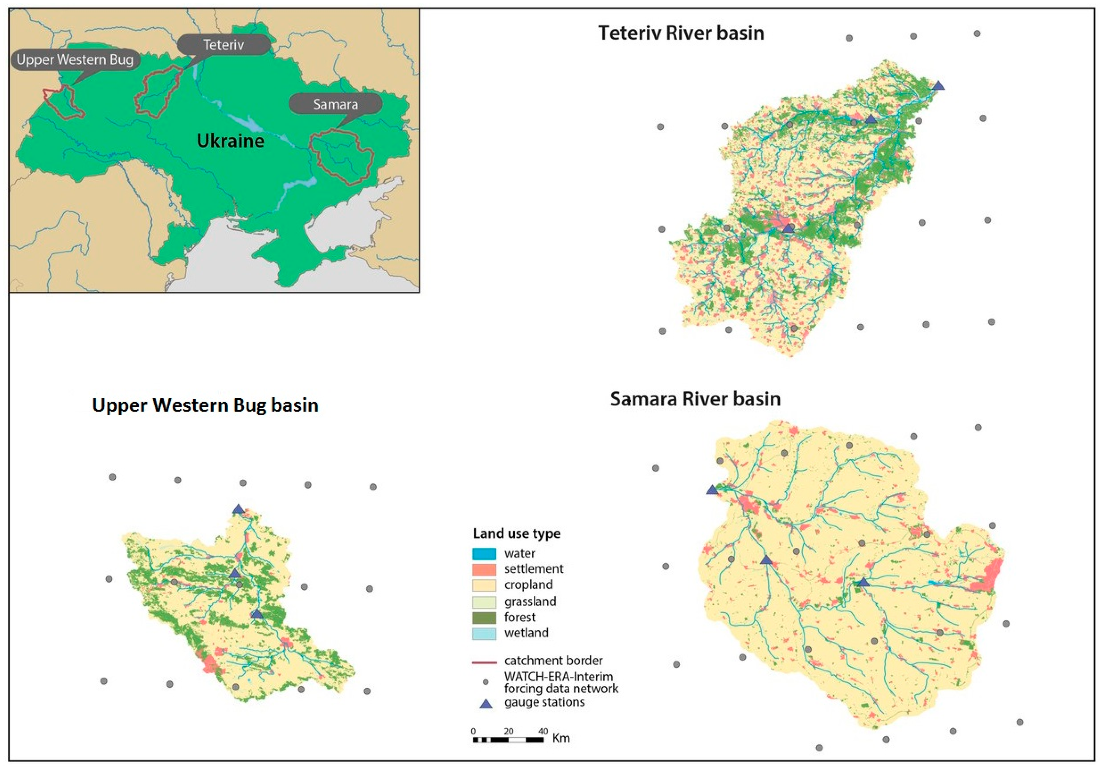
2.1. Study Area

Ukraine receives a large share of its surface water resources from other countries. Potential renewable water resources in Ukraine are 175.3 km³ per year [19], only 31% of which are formed in the country itself, and the rest comes from the Russian Federation, the Republic of Belarus, and the Danube River countries.

The total water withdrawal including cooling water for power plants in Ukraine has the following structure: on average, 88.6% from surface (river) water and 11.4% from groundwater [20]. Some European countries, like Poland, France, and Germany, have a similar structure of water consumption dominated by surface water [21].

The annual freshwater withdrawal from internal renewable water resources in Ukraine is 27%. The structure of water withdrawal by sector is: 30% for agriculture, 22% (3.27 billion m³·a⁻¹) for domestic use, and 48% (7.15 billion m³·a⁻¹) for industry. The total water withdrawal per capita is 327.7 m³·a⁻¹ [20].

The issues of water resources availability, management, and future changes are very important in Ukraine from the different aspects of sustainable development of the social, economic, and agricultural sectors. We aim to assess the potential water resources changes in Ukraine by considering representative areas in the northern, western, and southeastern parts of the country. Therefore, our research focuses on three mesoscale river catchments: the Teteriv, Samara, and Upper Western Bug (herein called “Western Bug”) (see Figure 1). They a have different geophysical, climate and hydrological conditions (

Table 1. The major characteristics of the basins under study (average annual temperature (T), precipitation (P), runoff (Q), and runoff coefficient (RC)).

	Teteriv	Samara	Western Bug
Total drainage area, km2	15,100	22,600	39,420
Drainage area considered in the modelling, km2	12,400	19,800	6,750
Gauging stations	Ivankiv,	Kocherizhki,	Lytovezh,
	Ukrainka,	Grushevskiy,	Mezhirichya,
	Zhitomir	Vasilkovka	Kamenka-Bugskaya
Major tributaries	Irsha, Guyva, Gnulopyat	Vovcha, Kilchen, Buk, Veluka Ternivka	Luga, Rata, Solokia
Q, m3/s	33.8	14.8	34.2
P, mm	621	535	682
T, °C	7.0	8.2	7.4
Runoff coefficient (RC)	0.14	0.04	0.23
Major land use types	Cropland 53%	Cropland 75%	Cropland 67%
	Forest 24%	Forest 13%	Forest 24.8%
	Settlements 12%	Settlements 7%	Settlements 4%

Note: The runoff coefficient (RC) is a ratio between the amount of runoff and the amount of precipitation, both averaged over a long period.

).

The Teteriv River is located in the northern part of Ukraine, and is one of the tributaries of the Dnipro River [22], which flows into the Black Sea. It has a total drainage area of about 15,100 km² covering three administrative regions. The river catchment with continental climate and soddy-podzolic soils is representative for this part of Ukraine. It is situated between wet west and cold east, and has notable shares of arable land (53%) and mixed forest (24%).

Another tributary of the Dnipro River and the object of our study, the Samara River, is located in the southeast of Ukraine. Its catchment, with the total drainage area of 22,600 km², covers two administrative regions. This river catchment is considered representative for the step region, it is characterized by fertile chernozems, warm climate, and flat topography. Additinally, the catchment is characterized by dry conditions (runoff coefficient of 0.04) and intensive land use by the agricultural sector.

The third river, Western Bug, is situated in the western part of Ukraine and is the left-bank tributary of the Narew River, which flows to the Baltic Sea. The Western Bug catchment is representative for this region. It has a wet climate, predominantly grey soils, and cropland (67%) and mixed forest (about 25%) as dominant land covers. In this study, we considered only the upper, Ukrainian part of the Western Bug catchment with the total area of about 6750 km². This catchment is the wettest of the three, and has the highest runoff coefficient of 0.24. The major characteristics of the basins are included in Table 1, where average annual temperature and precipitation are estimated for the period 1960–1990 [23], and river discharge for 1990–2010 [24].

All three catchments have relatively flat topography, with elevation ranges from 40 m a.s.l. (above sea level) to 480 m a.s.l. The river slopes range from 0.35 m/km in the Samara catchment to 0.61 and 0.69 m/km in the Teteriv and Upper Western Bug catchments, correspondingly. The annual mean precipitation increases from southeast to northwest, and ranges between 550 and 650 mm·a⁻¹ on average. The major land use types in the catchments are represented by cropland, forest, and settlements. The Samara has the highest coverage by cropland (75%), and the smallest area of forest (13%) among three catchments; the highest share of settlements is in the Teteriv catchment, while the Western Bug has the smallest share of them (4%). Table 1 summarizes the geophysical characteristics of three basins under consideration. Due to differences in geophysical and socio-economic conditions in the regions the water management strategies are also different.

Water consumption in the Teteriv and Samara basins consists of 90% of surface water and 10% of groundwater, which is close to the average for the whole country. Conversely, water consumption in the Western Bug basin consists of 98.5% of groundwater and 1.5% of surface water.

The annual water abstraction in the Teteriv basin is 157 mio·m³ on average, distributed among pond-fishing, industry, domestic uses, and agriculture. The catchment is characterized by a wide network of drainage canals and a large share of ameliorative land cover (about 20% of the cropland area). There are 54 reservoirs, each with volumes of more than 1 mio·m³, and the total volume of all reservoirs is 175.173 mio·m³ within the Zhytomyr administrative region [25].

The structure of water consumption in the Western Bug basin is similar. The largest part of water abstraction is taken for domestic uses, followed by industry, agriculture, and pond-fishing (17%). There are five reservoirs within the catchment with the total volume of 24.36 mio·m³, which is 2.2% of the average annual runoff [26].

Water consumption in the Samara catchment differs from the two other catchments due to its drier natural conditions and developed industry in this region. This catchment is located in the southeastern part of Ukraine, and has a wide irrigation network, which was created during 1960–1980. Each year about 9% of the total water consumption is used for irrigation. The major part of natural flow belongs to industry (about 60%), especially for water-intensive industries, such as power, metallurgy, and chemical sectors. Additionally, about 20% of water is used for domestic water withdrawal. Within the basin, there are 50 reservoirs with a total volume of 121.3 mio·m³, which is equal to 25% of the average annual runoff in the catchment [27].

Water management does not have a significant influence on the naturalized flow in the Teteriv and Western Bug catchments, as the percentage share of water abstraction in the total runoff of the catchment is small. Most of the water consumed is water for industries and domestic use, large volumes of which return to the surface water. However, the share of consumption is higher in the Samara catchment, and the role of abstracted water for irrigation purposes in this dry catchment is essential. Hence, implementation of water management in the modeling of this catchment could decrease uncertainty in the projections and improve the modelling in general.

However, due to data scarcity on water management in the case study basins, water management was not implemented in the modelling, and only natural flows were simulated.

2.2. SWIM Model Description

The Soil and Water Integrated Model (SWIM) is an eco-hydrological, partly empirical and partly process-based, model for simulation of the hydrological, vegetation and nutrient cycle processes at the river basin scale. SWIM is based on two previously-developed models: SWAT [28] and MATSALU [29]. The MATSALU model was developed in Estonia for the agricultural basin of the Matsalu bay to evaluate different management scenarios for eutrophication control of the bay. SWAT is a continuous-time semi-distributed watershed model, developed to predict the effects of alternative land management decisions on water, sediments and chemical yields. Detailed information on the SWAT model can be found in Arnold et al. [28].

SWIM simulates hydrological processes, vegetation growth, sediment transport and nutrient cycling at the river basin scale using topographic, land use, soil, climate and vegetation input data as underlying datasets. The model uses a three-level disaggregation scheme: basin—sub-basins—hydrotopes (or hydrological response units, HRU). The hydrotopes are homogenous spatial sets of units within sub-basins obtained by overlaying of sub-basin, soil and land use maps. Runoff generation is approached by the well-known curve number (CN) method, which is an empirical approach reflecting direct runoff coefficients for different land surfaces, depending on soil parameters, land cover, and soil water content [30]. The budgeting of the hydrological processes in the model is based on the water balance equation. The control volumes considered are: soil surface, root zone in soil profile, shallow aquifer, and deep aquifer. In the crop and vegetation module the Erosion Productivity Impact Calculator (EPIC) [31] approach is utilized, which applies specific parameter values for each crop and vegetation type. More detailed information on the model can be found in Krysanova et al. [18].

In recent years, the SWIM model has been applied for many river basins in Europe, Africa, Asia, and South America [32,33,34,35,36]. The modelling was focused not only on hydrological issues, but also on sediments, extreme events, crop yield, and water quality [37]. Some modules were improved, like the snow module, or added for specific applications, such as the wetland module, reservoir module, glacier module, etc.

2.3. Input Data

To set up the SWIM model, the digital elevation model (DEM), land use map, soil map and its parametrization, and climate data are all required. SWIM operates on a daily time step and is driven by the following daily climate data: precipitation, minimum, maximum, and mean temperatures, solar radiation, and relative humidity.

For this study, a digital elevation model derived from the Shuttle Radar Topography Mission (SRTM) of The CGIAR Consortium for Spatial Information (CGIAR-CSI) was applied. The spatial resolution of the SRTM data is 90 × 90 m [38].

Land use input data were combined from data obtained from open sources [39,40,41], and by classification of satellite images based on Landsat 5 [42], with further reclassification to the 15 land use categories needed in SWIM (water, settlement, industry, road, bare soil, cropland, meadow, pasture, set-aside, evergreen forest, deciduous forest, mixed forest, wetland, heather, and glaciers). The land use information derived from satellite data covers the period between 2004 and 2007 years. The land use classes were obtained by combining three different bands, and a further re-classification. All land use data was considered as homogeneous for all simulated periods, as usually done in climate impact studies. The agricultural sector, due to fertile soils, was one of the most developed sectors in Ukraine, but in the 1990s industrial farming had a recession that led to some changes in land use composition. In recent years, the agricultural sector shows a stable increase.

The soil map and parameterization of soil layers (clay, silt, sand, bulk density) were obtained from the Harmonized World Soil Database [43] created by the Food and Agriculture Organization of the United Nations, and reformatted for SWIM. Other parameters of soil profiles (porosity, available water capacity, field capacity, erodibility factor, and saturated conductivity) were estimated by the pedotransfer functions [44].

Regarding climate data from meteorological stations located in the catchments, the main problems were the low density of the observation stations and, partly, the unsatisfactory quality and low accessibility of the data. There were several gaps in the observation time series, and some essential parameters were not available. Therefore, it was decided to derive climate data for the modelling from WATCH Forcing Data ERA Interim (called WFDEI) [45]. These meteorological data were obtained from the European Centre for Medium Range Weather Forecasting. WFDEI was produced with the same methodology as WATCH Forcing Data [46] applied to ERA-Interim reanalysis data [47]. It is a meteorological forcing dataset extending into the early 21st century for the period 1979–2012, with regular spatial resolution grid (0.5° × 0.5°).

The daily river discharge data for hydrological gauges within the considered catchments were obtained from the Ukrainian Hydrometeorological Center [24].

2.4. Model Setup, Calibration, and Validation

For calibration of the model, observed river discharge data from the hydrological gauges Ivankiv (Teteriv), Kocherizhki (Samara) and Lytovezh (Western Bug) were used. The Kocherizhki and Ivankiv gauges are located close to the outlets of the catchments, and Lytovezh is close to the Ukrainian–Polish border. Different time periods of different lengths were chosen for calibration and validation for each basin, subject to data availability. The Teteriv River basin was calibrated and validated for the period 1999–2009, Samara for the period 1992–2004, and Western Bug for the period 1995–2004. In all cases approximately half a period was taken for calibration, and the rest used for validation. Moreover, for validation of the model discharge data at two additional gauges within each catchment were compared to simulated values.

During the calibration of the model a number of parameters affecting runoff (CN), infiltration (saturated conductivity and field capacity), evaporation (correction factors in the Priestley-Taylor method), groundwater (initial groundwater flow contribution to streamflow, alpha factor, groundwater delay, and baseflow factor), snow melt (threshold temperature and rate of snow melt, threshold temperature of snow fall), and routing were adjusted (but not all in every case). The most sensitive parameters for all basins under consideration during the process of calibration were correction parameters for snow melt (since discharge in all rivers under study is partly influenced by snowmelt), curve numbers, evaporation and groundwater.

The Nash-Sutcliffe efficiency coefficient [48] and percent bias were used to evaluate the model performance and successfulness of model calibration. The Nash-Sutcliffe efficiency (NSE) is a normalized statistic that determines the relative magnitude of the residual variance (“noise”) compared to the measured data variance (“information”) ranging from −∞ to 1, where values from 0.7 to 1 correspond to satisfactory calibration results (according to Moriasi et al. [49]), and 1 indicates a perfect fit. Percent bias (PBIAS) measures the average tendency of the simulated data to be larger or smaller than their observed counterparts [50]. The values of PBIAS higher than 0 are defined as underestimation, and negative values as overestimation. It was assumed that the PBIAS values in the range between ±15% indicate a good model performance (based on Moriasi et al. [49]).

2.5. Climate Scenarios

Climate scenarios were derived from the FP7-funded IMPRESSIONS project (Impacts and Risks from High-End Scenarios: Strategies for Innovative Solutions) [51]. The climate projections constitute a set of seven GCM-RCMs coupled climate simulations with 0.5° resolution under RCP 4.5 and RCP 8.5 forcings until 2100. The RCP 2.6 and RCP 6.0 pathways were not considered in IMPRESSIONS, as well as in our study. These GCM/RCM projections were selected to cover the range of projected temperature increases in Europe, which vary according to the RCP forcing as well as to model sensitivity [51]. The climate simulations were obtained from the CORDEX database and bias-corrected in the IMPRESSIONS project to the WFDEI dataset.

These seven climate projections were combined in IMPRESSIONS into three sets of low, intermediate, and high-end scenarios. The high-end scenarios include three projections under RCP 8.5: HadGEM2-ES/RCA4, CanESM2/CanRCM4, and IPSL-CM5A-MR/WRF. The intermediate scenarios include the GFDL-ESM2M/RCA4 scenario under RCP 8.5 and the HadGEM2-ES/RCA4 scenario under RCP 4.5. The low-end scenarios include two projections under RCP 4.5: GFDL-ESM2M/RCA4 and MPI-ESM-LR/CCLM [52]. An empirical statistical quantile mapping method was used for bias correction [53]. This method performed well compared to other bias correction methods [54]. Each variable was calculated independently. For bias-correction, the period from 1981 to 2010 was taken, because WFDEI data is available for 1979–2012, historical GCM/RCM series are available up to 2005, and for the period 2006–2010, RCP 4.5 simulations were used. Regarding the potential RCP influence, the difference between RCP 4.5 and RCP 8.5 in 2006–2010 is very small, and the effect is negligible.

Some GCM/RCM simulations extend only until 2098 or 2099. The climate scenario datasets include the following variables: maximum, minimum, and mean temperature, daily precipitation, shortwave radiation, wind speed, and relative humidity.

To estimate climate change induced signals of changes in river runoff, the period from 1981 to 2010 was taken as a reference period (corresponding to the bias-correction period), and the future period was subdivided into three time slices: near future, 2011–2040; middle future, 2041–2070; and far future, 2071–2100—simulations for which were later compared to those in the reference period. The signals of air temperature change in the three chosen scenario sets in our three basins vary from 0.9 to 1.6 in the low-end scenarios, from 1.1 to 3.2 in the intermediate scenarios, and from 1.1 to 4.7 in the high-end scenarios, and increase from the near future to the end of the century (see

Table 2. The long-term average temperature, precipitation and river discharge: absolute values in four periods and delta changes in the scenario periods related to the reference period for the three catchments under study.

Catchment	Period	T, °C			ΔT, °C			P, mm			ΔP, mm			Q, mm			ΔQ, mm
		L	I	H	L	I	H	L	I	H	L	I	H	L	I	H	L	I	H
Teteriv	reference	8.2	8.2	8.2				658	666	664				79	84	79
	near	9.3	9.4	9.4	1.1	1.2	1.2	655	714	714	−3	48	50	81	107	102	−0.5	7.2	7.5
	middle	9.6	10.7	10.8	1.4	2.5	2.6	674	691	751	16	25	87	86	89	114	2.4	3.8	13.1
	far	9.8	11.4	12.6	1.6	3.2	4.3	654	695	765	−4	29	101	81	107	119	−0.6	4.4	15.2
Upper Western Bug	reference	8.1	8.1	8.1				738	757	743				180	188	188
	near	9	9.1	9.2	0.9	1.1	1.1	729	809	796	−9	52	53	178	228	227	−1.2	7.1	7.1
	middle	9.4	10.3	10.5	1.3	2.3	2.4	749	791	822	11	34	79	198	214	246	1.5	10.6	10.6
	far	9.6	10.9	12.3	1.5	2.9	4.2	748	811	862	10	54	119	196	259	301	1.4	16	16
Samara	reference	9.3	9.3	9.3				583	589	580				44	40	35
	near	10.2	10.4	10.6	0.9	1.2	1.3	577	598	619	−6	9	39	40	49	48	−1	1.5	6.7
	middle	10.7	11.6	12.2	1.4	2.3	2.9	573	587	636	−10	−2	56	45	46	48	−1.7	−0.3	9.7
	far	10.9	12.5	14	1.5	3.2	4.7	555	569	662	−28	−20	82	46	37	60	−4.8	−3.4	14.1

Scenarios: L—low-end, I—intermediate, H—high-end. Periods: reference (1980–2010), near (2011–2040), middle (2041–2070), and far (2070–2100).

).

3. Results

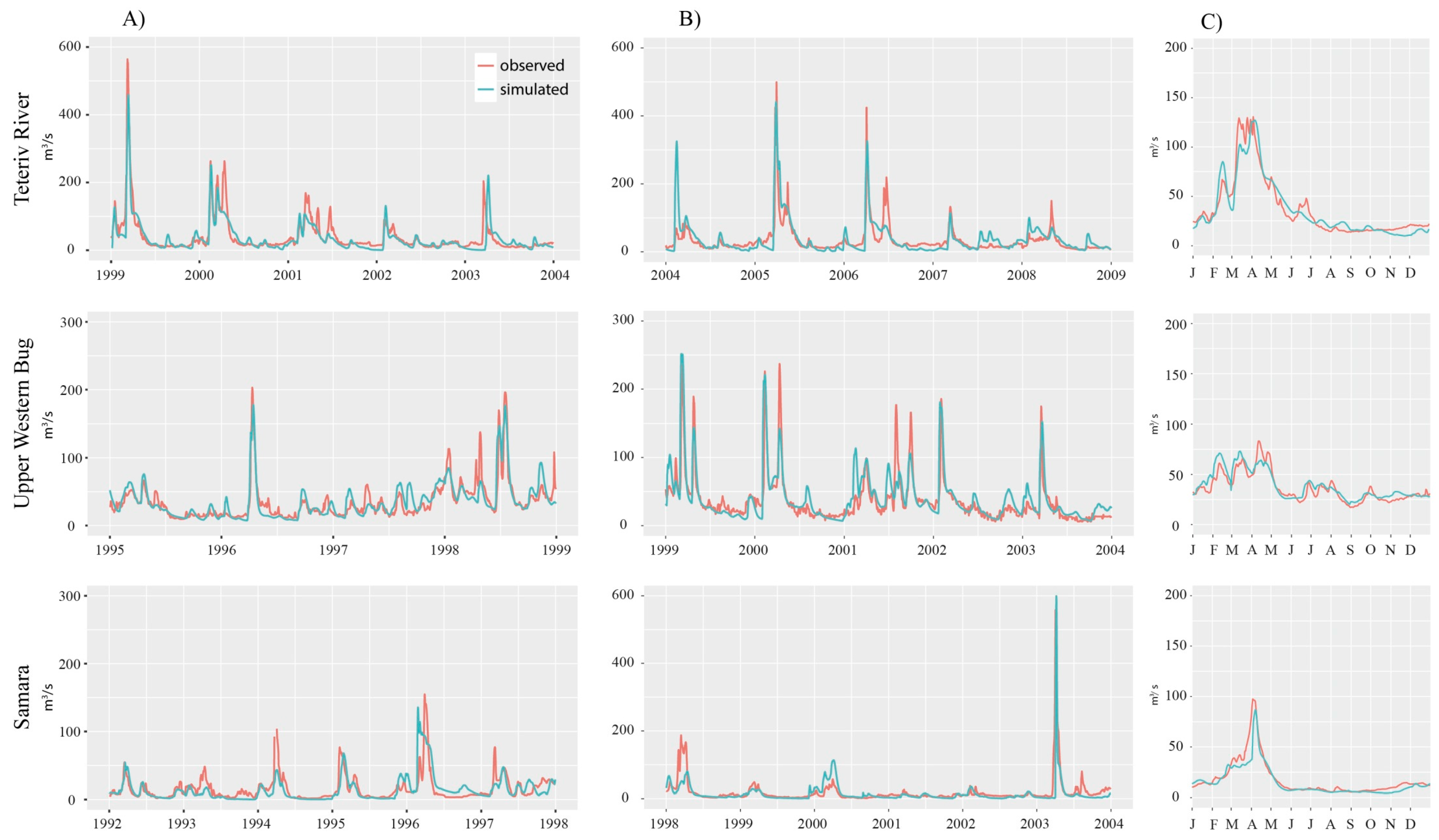
3.1. Model Performance

All three catchments are characterized by high flow in spring due to snow (accumulated during winter) melting. The summer months in the Teteriv and Samara basins are quite dry, and characterized by low flow in this period. The SWIM model was able to represent the daily runoff in the three river catchments under consideration. Figure 2 and

Table 3. Results of calibration and validation of the model with the daily and monthly time steps in terms of two criteria: NSE—Nash-Sutcliffe efficiency, and Pbias—Percent bias.

Catchment	Calibration				Validation
	NSE		Pbias		NSE		Pbias
	Daily	Monthly	Daily	Monthly	Daily	Monthly	Daily	Monthly
Teteriv (Ivankiv)	0.75	0.82	−10.8	−10.5	0.53	0.57	9.5	10
Upper Western Bug (Lytovezh)	0.75	0.82	1.8	3.3	0.67	0.76	10.2	12
Samara (Kocherezhky)	0.42	0.5	−3.9	−11.9	0.58	0.71	−21	−21.3

illustrate the results of calibration and validation of the model. the simulation results for all catchments and periods vary from “satisfactory” to “very good” (according to the Moriasi and Arnold classification [49]). The long-term average seasonal discharge with the daily time step is also in good agreement with the observed time series.

One of the main problems during calibration was the lack of water management data. Due to this, it was not possible to include reservoirs and irrigation demands in the simulation runs and, hence, it was difficult to reproduce river runoff accurately, especially in the intensively-managed Samara catchment (e.g., in March and April during spring floods, and in summer during the low flow period when irrigation is applied).

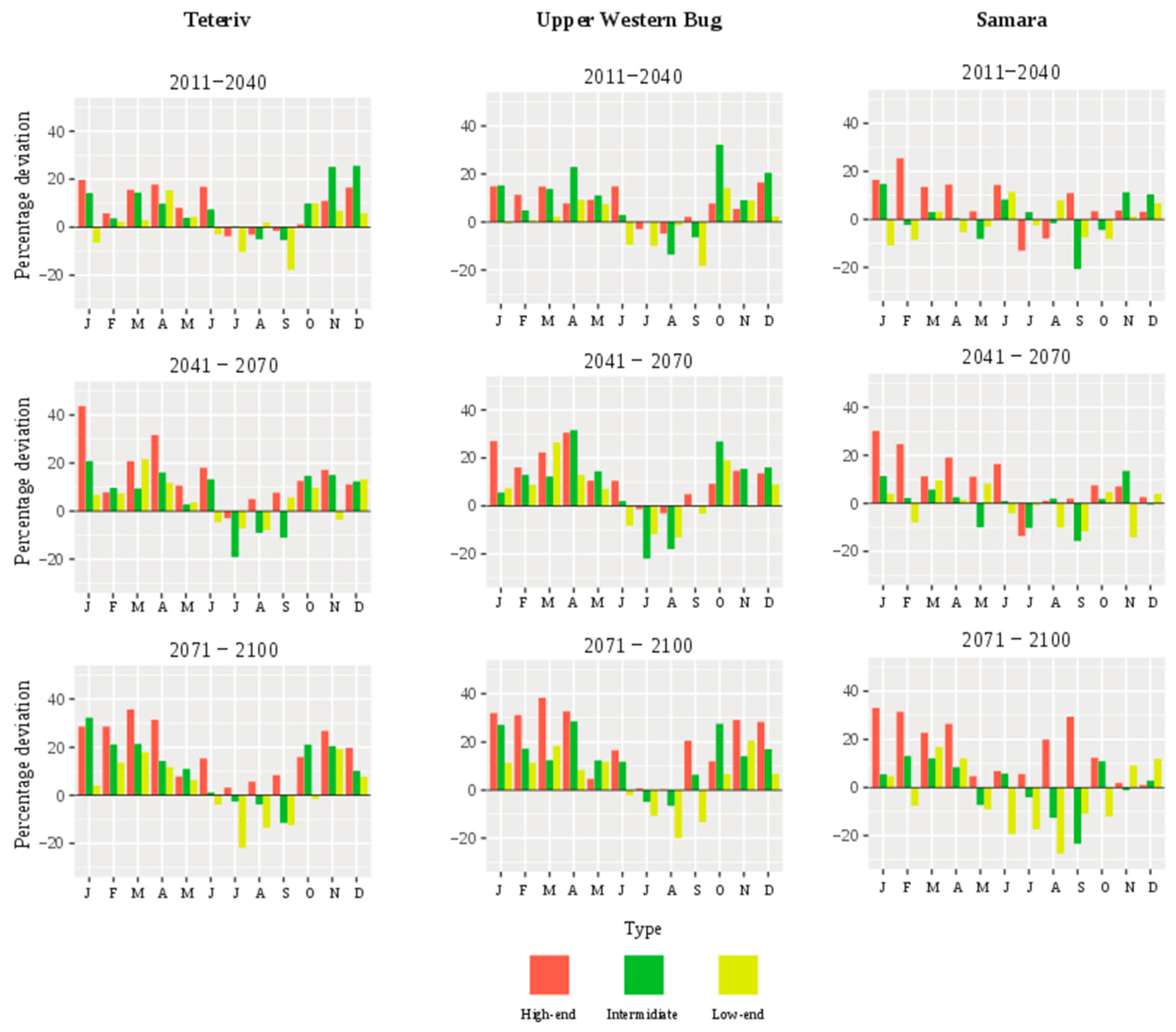
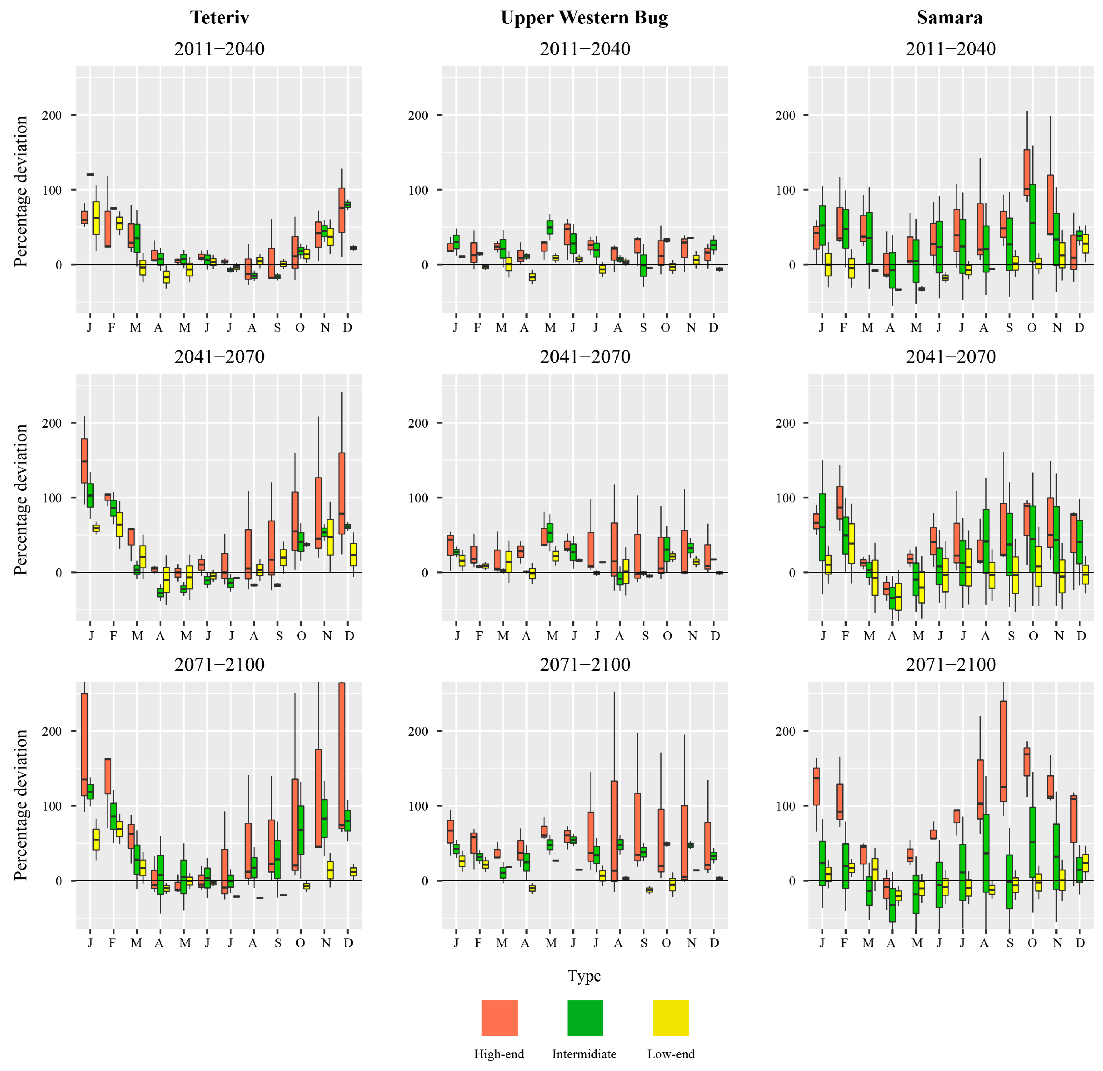
3.2. Assessment of Expected Climate Change Impacts

The projected annual average temperature shows gradual increases for all catchments until the end of the century. In all basins air temperature increases more intensively under the high-end scenarios in comparison to the low-end and intermediate ones. In the Teteriv River basin the average annual temperature rises from +8.2 °C in the period 1981–2010 to +9.8 °C at the end of the century under the low-end scenarios, up to +11.4 °C under the intermediate scenarios, and up to +12.6 °C under the high-end scenarios. In the same way, the average annual temperature rises in the Western Bug catchment from +8.1 °C in the reference period to +9.6 °C under the low-end scenarios, up to +10.9 °C under the intermediate scenarios, and up to +12.3 °C under the high-end scenarios at the end of the century. In the Samara catchment the average annual temperature rises from +9.3 °C in the reference period to +10.9 °C under the low-end scenarios, up to +12.5 °C under the intermediate scenarios, and up to +14 °C under the high-end scenarios at the end of the century (Table 2).

Regarding precipitation, the mean annual precipitation shows an increasing trend under intermediate and high-end scenarios for the Teteriv and Western Bug catchments, as indicated by the multi-model mean: in the Teteriv catchment, up to 15%; and in the Western Bug, up to 16%. The precipitation under the low-end scenarios shows insignificant increases up to 2%, with sporadic decreases up to 1% in the near future. In the Samara catchment the mean annual precipitation shows a decrease of up to 4% under the low-end scenarios, up to 3% under the intermediate scenarios, and increases up to 14% under the high-end scenarios at the end of the century.

More significant changes occur in the distribution of precipitation during the season. The seasonal dynamics of changes show a clear rise in winter and fall months up to 40% under all scenarios, and decreases in the summer season, mostly under the low-end and intermediate scenarios for the Teteriv and Western Bug catchments (Figure 3). The Samara basin is characterized by some disagreement in signals between scenarios and periods, especially from late spring to the end of the year. From January to April precipitation increases up to 30% for all future periods under the intermediate and high-end scenarios. The last period shows a decrease in precipitation under the low-end scenarios from spring to early fall, and an opposite signal under the high-end scenarios.

Changes in seasonal dynamics of river discharge for three future periods, compared to the reference period in the catchments under study, are presented in Figure 4. The Teteriv catchment is characterized by an increase in discharge in winter months and early spring for all future periods. In the reference period the highest river discharge occurs in March and April, driven by snow melting. In the projections for future periods snow melting shifts to the earlier months, and the highest peak of discharge occurs in March. In summer months river discharge remains approximately the same in the near future, but in the middle and far future periods small decreases of discharge (up to 17%) are possible. Additionally, increases in discharge were projected in August for the middle and far future time slices under the intermediate and high-end scenarios. The fall months are characterized by stable increases of river discharge practically for all time periods and scenarios, except some decreases of river discharge in early fall for the low-end and intermediate scenarios. The simulations corresponding to the high-end scenarios show higher rises and wider ranges of uncertainty, compared to the low-end and intermediate scenarios in autumn and winter months.

The river discharge of the Western Bug is projected to have a steady rise during all seasons (with some small sporadic decreases in spring months in the near and far future) under all scenarios compared to the reference period. The far future period shows a higher rise of discharge during all seasons under the high-end scenarios, with the higher ranges of uncertainty (for 25th–75th percentiles) varying from +5% to +110% in July–December months, compared to the previous time periods. The river discharge under the low-end and intermediate scenarios shows increases during the whole year with some small sporadic decreases. The increases in river runoff in summer and fall months, even under precipitation decrease in these months, could be explained by a delayed runoff due to a high level of groundwater in the earlier period.

The results obtained for the Samara river basin show wide ranges of uncertainty under high-end and intermediate scenarios. The changes in seasonal dynamics of river discharge are quite similar for all three periods. The river runoff increases in virtually all months during winter, summer, and fall under the high-end scenarios in all future periods. In April all scenarios show decreases of river runoff. The high-end scenarios show the highest values compared to two other scenarios, especially in the far future. The river discharge under the low-end scenarios shows decreases in March–July and increases in November and December in the near future, decreases in spring season in the middle future, and decreases from April to September and increases in the winter season in the far future.

4. Discussion

The projected changes in climate can lead to adverse effects on water resource availability and stability which, in turn, could affect different economic and social sectors. A comprehensive assessment of future changes is crucial for regional water resource planning. Therefore, such information, as well as the evaluation of risks associated with impacts, have to be accounted for in the integrated water management plans. The identification of adaptation measures for the water sectors, including the ‘no-regret’ or ‘win-win’ solutions strategies can be founded based on such studies, even though the associated uncertainties appear to be high.

The main goal of our research was to investigate potential climate change impacts on river discharge for three catchments in different parts of Ukraine. The projected changes were evaluated by the end of the century, using ecohydrological model SWIM and seven climate scenarios corresponding to RCPs 4.5 and 8.5 from the IMPRESSIONS project.

According to the IPCC assessment report [2], projected changes in precipitation in Europe differ regionally and seasonally. For proper assessment of climate change impacts on water resources, it is important to have global, as well as, regional-scale assessments. Considering that a vast amount of such studies for river basins and countries in Europe have been carried out, it is surprising that not many country-scale or river basin studies have been performed for Ukraine. Previously, studies focusing on the assessment of potential climate impacts on river discharge for this region used different approaches, and sometimes had opposite results. Mostly, they used a small number of scenarios and a simple water balance method instead of applying a hydrological model. In some cases it is hard to compare the results due to different reference and future periods. Additionally, the reason for the differences in results can be the climate models that were used and their sensitivity to emission scenarios.

In our study, and with this paper, we have tried to overcome the deficiencies of previous studies, and applied a state-of-the-art ecohydrological model driven by seven recently-developed climate scenarios for two RCPs. Additionally, an important step was to choose representative river catchments within different geographical zones of Ukraine, and to assess changes in a catchment with dry conditions having small runoff coefficient (Samara River) and also in two catchments with wetter conditions (Teteriv and Western Bug catchments).

Our results revealed a stable increase in temperature and changes in precipitation during the year for all river basins considered. The most pronounced finding is the shifts in the seasonal distribution of runoff in all three basins. The spring high flow occurs earlier as a result of temperature increases and earlier snowmelt in all catchments under consideration. A fairly robust trend of increases in river discharge in the winter season is found in all three catchments, caused by increases in precipitation and, possibly, earlier snow melting as a result of higher temperatures, a trend with which the majority of the projections agreed. Moreover, most scenarios show a potential reduction in discharge in spring, accompanied by a shift of the spring peak to earlier months. The similar trends in seasonal dynamics were found in the study of Čerkasova et al. and Hesse et al. [13,55] with increases to the river discharge in winter and decreases in spring as a result of temperature rises. Additionally, in some cases the maximum spring discharges take place earlier.

However, during the fall–winter season, when significant increases in mean river discharge are projected, there are wide ranges of uncertainty, especially for the Teteriv and Samara catchments. Basically, the projections agreed on the direction of change for the Teteriv and Western Bug, but the rates of change varied significantly among the scenarios. Spring months are characterized by the shifting of the spring flood peak to an earlier period, as a result of warming in the winter season. An increase in temperature and decrease in precipitation during the summer months could lead to a decrease in river runoff for the middle and far future periods in the Teteriv catchment.

In the Western Bug no straightforward response to monthly precipitation was found, showing an increase in discharge in summer despite reduced precipitation, and only a minor reduction in some of the summer months under the low-end scenarios. This can be explained by the higher level of groundwater in this catchment due to the larger amount of precipitation in the winter and spring seasons under climate change. The potential evapotranspiration increases in the Western Bug catchment during the year as a result of temperature increases. The same trend shows the actual evapotranspiration in winter, but in summer, as result of precipitation decrease and temperature increase, the actual evapotranspiration shows a decrease in all scenarios.

On the other hand, in the Samara catchment there is a clear correlation between the increased precipitation and river discharge in the summer season under the high-end scenarios, and decreases in both under the low-end scenarios in the far future.

Considering the uncertainty of the projections in river discharge in three catchments under study, it should be mentioned that in the Teteriv catchment the high-end scenarios yield the highest range of uncertainty in comparison to the low-end and intermediate scenarios, which increase from near to far future period. There are also some differences in seasonal dynamics, in winter and fall seasons the uncertainty is higher compared to the summer season. The Western Bug shows the lowest range of uncertainty compared to the other catchments. The high-end scenarios yield higher uncertainty ranges from July to December in the middle and far future, compared to the near future. The Samara catchment is characterized by the highest range of uncertainty among all considered catchments. All future periods have a wide range of uncertainty for high-end and intermediate scenarios. The low-end scenarios show small uncertainty ranges compared to the other scenarios, but increase in the middle future.

The three basins considered in this study, especially the Samara and Teteriv River basins, play important roles in the socio-economic development of the administrative regions. Due to potential future changes in discharge and hydrological regimes of these river basins, it is necessary to develop adaptive measures in water management and for social and other related economic sectors. Especially, it is important to adapt the seasonal regime of water consumption and distribution for different purposes in the regulated subcatchments with large numbers of reservoirs.

5. Conclusions

Ukraine is one of the largest countries in Europe with a high scientific potential. However, the assessment of climate change impacts on water resources is not yet developed at a sufficient level and many more investigations in this direction are needed. Future changes can affect different sectors—industry, agriculture, food production, and development of the regions, themselves, directly or indirectly, and may lead to undesirable consequences. Therefore, it is necessary to have projections of potential future changes, which could be helpful for creating a strategy of sustainable development on different scales.

In this paper we considered two tributaries of the Dnipro River, but a complex assessment of potential changes in the whole Dnipro River basin would be of interest as it is the largest and most important river in Ukraine and one of the largest rivers in Europe. It is a regulated river with a high water use for hydropower, irrigation, and domestic consumption. Thus, changes in the hydrological regime of the river can lead to serious consequences, and should be investigated in the future.

The largest share of the drainage areas in all three representative catchments under study is used by agriculture. Intensive agriculture can lead to nutrient pollution, eutrophication of water bodies, and a decline in water quality. Additionally, the high consumption of water for industrial purposes and its return in surface waters can lead to temperature pollution and negative environmental effects in the rivers. Furthermore, the important issue is poor availability and, in some cases, lack of water management data in the river catchments. The implementation of water management in the modelling in the future could decrease the uncertainty of projections, and could help to develop adaptive measures. These aspects also deserve the attention of researchers. Equally important is studying climate change impacts on extremes: floods and low flows, together with the important additional drivers of potential land use changes (e.g., such as deforestation).

References

1. Bates, B.C.; Kundxewicz, Z.W.; Wu, S.; Palutikof, J.P. Climate Change and Water; Technical Paper of the Intergovernmental Panel on Climate Change; IPCC Secretariat: Geneva, Switzerland, 2008. [Google Scholar]
2. Kovats, R.S.; Valentini, R.; Bouwer, L.M.; Georgopoulou, E.; Jacob, D.; Martin, E.; Rounsevell, M.; Soussana, J. Climate Change 2014: Impacts, Adaptation, and Vulnerability. Part B: Regional Aspects. Contribution of Working Group II to the Fifth Assessment Report of the Intergovernmental Panel on Climate Change; Cambridge Univ. Press: Cambridge, UK, 2014; pp. 1267–1326. [Google Scholar]
3. Vormoor, K.; Lawrence, D.; Heistermann, M.; Bronstert, A. Climate change impacts on the seasonality and generation processes of floods—Projections and uncertainties for catchments with mixed snowmelt/rainfall regimes. Hydrol. Earth Syst. Sci. 2015, 19, 913–931. [Google Scholar] [CrossRef]
4. Cisneros, J.; Oki, T.; Arnell, N.W.; Benito, G.; Cogley, J.G.; Döll, P.; Jiang, T.; Mwakalila, S.S. Climate Change 2014: Impacts, Adaptation, and Vulnerability. Part A: Global and Sectoral Aspects. Contribution of Working Group II to the Fifth Assessment Report of the Intergovernmental Panel on Climate Change; Cambridge Univ. Press: Cambridge, UK, 2014; pp. 229–269. [Google Scholar]
5. European Commission The EU Water Framework Directive—Integrated River Basin Management for Europe. Available online: http://ec.europa.eu/environment/water/water-framework/index_en.html (accessed on 3 November 2016).
6. The World Bank Group. Renewable Internal Freshwater Resources per Capita (Cubic Meters). Available online: http://data.worldbank.org/indicator/ER.H2O.INTR.PC (accessed on 5 May 2016).
7. Snizhko, I.; Kuprikov, O.; Shevchenko, P.; Evgen, I.D. Use of Water-Balance Turk Model and Numerical Regional Model REMO for Assessment of Local Water Resources Runoff in Ukraine in the XXI Century; Bryansk State Univ. Her.: Bryansk, Russia, 2014; pp. 191–201. (In Russian) [Google Scholar]
8. Buksha, I.; Gozhik, P.; Iemekianova, Z.; Trifimova, I.; Shereshevskiy, A. Ukraine and Global Greenhouse Effect. Book 2. Vulnerability and Adaptation Ecological and Economical Systems to Climate Change; Agency for Rational Energy and Ecology Use: Kyiv, Ukraine, 1998. (In Ukrainian) [Google Scholar]
9. Loboda, N.; Serbova, Z. Modelling of Climate Changre Impact on the Rivers Flow of Ukraine. Impact Clim. Chang. Econ. Ukr. 2015, 1, 451–482. (In Ukrainian) [Google Scholar]
10. Bär, R.; Rouholahnejad, E.; Rahman, K.; Abbaspour, K.C.; Lehmann, A. Climate change and agricultural water resources: A vulnerability assessment of the Black Sea catchment. Environ. Sci. Policy 2015, 46, 57–69. [Google Scholar] [CrossRef]
11. Fischer, S.; Pluntke, T.; Pavlik, D.; Bernhofer, C. Hydrologic effects of climate change in a sub-basin of the Western Bug River, Western Ukraine. Environ. Earth Sci. 2014, 72, 4727–4744. [Google Scholar] [CrossRef]
12. Schneider, C.; Laizé, C.L.R.; Acreman, M.C.; Flörke, M. How will climate change modify river flow regimes in Europe? Hydrol. Earth Syst. Sci 2013, 17, 325–339. [Google Scholar] [CrossRef] [Green Version]
13. Hesse, C.; Stefanova, A.; Krysanova, V. Comparison of Water Flows in Four European Lagoon Catchments under a Set of Future Climate Scenarios. Water 2015, 7, 716–746. [Google Scholar] [CrossRef]
14. Pluntke, T.; Barfus, K.; Myknovych, A.; Bernhofer, K. Hydrologic Effects of Climate Change in the Western Bug Basin. In Proceedings of the Global and Regional Climate Changes, Kyiv, Ukraine, 16–19 November 2010.
15. Pluntke, T.; Pavlik, D.; Bernhofer, C. Reducing uncertainty in hydrological modelling in a data sparse region. Environ. Earth Sci. 2014, 72, 4801–4816. [Google Scholar] [CrossRef]
16. Tavares Wahren, F.; Helm, B.; Schumacher, F.; Pluntke, T.; Feger, K.-H.; Schwärzel, K. A modeling framework to assess water and nitrate balances in the Western Bug river basin, Ukraine. Adv. Geosci. 2012, 32, 85–92. [Google Scholar] [CrossRef] [Green Version]
17. Snizhko, S.; Yazuk, M.; Kuprikov, I.; Shevchenko, O.; Strutinska, V.; Krakovska, S.; Palamarchuk, L.; Shedemenko, I. Assessment of possible water resources changes of local runoff in Ukraine in XXI century. Water Econ. Ukr. 2012, 6, 5–20. (In Ukrainian) [Google Scholar]
18. Krysanova, V.; Wechsung, F.; Arnold, J.; Ragavan, S.; Williams, J. SWIM (Soil and Water Integrated Model), User Manual; PIK Report Nr. 69: Potsdam, Germany, 2000. [Google Scholar]
19. Ukraine—Water Management. Available online: http://www.fao.org/countryprofiles/index/en/?iso3=UKR&paia=4 (accessed on 2 November 2016).
20. AQUASTAT—FAO’s Information System on Water and Agriculture. Available online: http://www.fao.org/nr/water/aquastat/countries_regions/UKR/index.stm (accessed on 3 September 2016).
21. Eurostat. Available online: http://ec.europa.eu/eurostat (accessed on 3 September 2016).
22. Snizhko, S. Wasserwirtschaftliche und ökologische Situation im Dnipro—Einzugsgebiet. Hydrol. Wasserbewirtsch. 2001, 1, 2–8. [Google Scholar]
23. Climate Cadastre of Ukraine; Ukrainian Hydrometeorological Center: Kyiv, Ukraine, 2006. (In Ukrainian)
24. Ukrainian Hydrometeorological Center. Available online: http://meteo.gov.ua/en/ (accessed on 12 September 2015).
25. Regional Report on the State of the Environment in Zhytomyr Region in 2014; Department of Ecology and Natural resources of Zhytomyr Regional State Administration: Zhytomyr, Ukraine, 2015. (In Ukrainian)
26. Regional Report on the State of the Environment in Lviv Region in 2014; Department of Ecology and Natural resources of Lviv Regional State Administration: Lviv, Ukraine, 2015. (In Ukrainian)
27. Regional Report on the State of the Environment in Dnipropetrovsk Region in 2014; Department of Ecology and Natural resources of Dnipropetrovsk Regional State Administration: Dnipropetrovsk, Ukraine, 2015. (In Ukrainian)
28. Arnold, J.G.; Fohrer, N. SWAT2000: Current capabilities and research opportunities in applied watershed modelling. Hydrol. Process. 2005, 19, 563–572. [Google Scholar] [CrossRef]
29. Krysanova, V.; Meiner, A.; Roosaare, J.; Vasilyev, A. Simulation modelling of the coastal waters pollution from agricultural watersched. Ecol. Model. 1989, 49, 7–29. [Google Scholar] [CrossRef]
30. Arnold, J.; Williams, J.; Nicks, A.; Sammons, N. SWRRB–A Basin Scale Simulation Model for Soil and Water Resources Management; Texas A&M University Press: College Station, TX, USA, 1990. [Google Scholar]
31. Williams, J.R.; Renard, K.G.; Dyke, P.T. EPIC—A new model for assessing erosion’s effect on soil productivity. J. Soil Water Conserv. 1984, 38, 381–383. [Google Scholar]
32. Hattermann, F.F.; Post, J.; Krysanova, V.; Conradt, T.; Wechsung, F. Assessment of Water Availability in a Central-European River Basin (Elbe) under Climate Change. Adv. Clim. Chang. Res. 2008, 4, 42–50. [Google Scholar]
33. Huang, S.; Krysanova, V.; Zhai, J.; Su, B. Impact of Intensive Irrigation Activities on River Discharge Under Agricultural Scenarios in the Semi-Arid Aksu River Basin, Northwest China. Water Resour. Manag. 2014, 29, 945–959. [Google Scholar] [CrossRef]
34. Aich, V.; Liersch, S.; Vetter, T.; Huang, S.; Tecklenburg, J.; Hoffmann, P.; Koch, H.; Fournet, S.; Krysanova, V.; Müller, E.N.; et al. Comparing impacts of climate change on streamflow in four large African river basins. Hydrol. Earth Syst. Sci. 2014, 18, 1305–1321. [Google Scholar] [CrossRef] [Green Version]
35. Stagl, J.; Hattermann, F. Impacts of Climate Change on the Hydrological Regime of the Danube River and Its Tributaries Using an Ensemble of Climate Scenarios. Water 2015, 7, 6139–6172. [Google Scholar] [CrossRef]
36. Lobanova, A.; Stagl, J.; Vetter, T.; Hattermann, F. Discharge alterations of the Mures River, Romania under ensembles of future climate projections and sequential threats to aquatic ecosystem by the end of the century. Water 2015, 7, 2753–2770. [Google Scholar] [CrossRef]
37. Krysanova, V.; Hattermann, F.; Huang, S.; Hesse, C.; Vetter, T.; Liersch, S.; Koch, H.; Kundzewicz, Z.W. Modelling climate and land-use change impacts with SWIM: Lessons learnt from multiple applications. Hydrol. Sci. J. 2015, 60, 606–635. [Google Scholar] [CrossRef]
38. CGIAR-CSI SRTM 90m DEM Digital Elevation Database. Available online: http://srtm.csi.cgiar.org/ (accessed on 5 November 2015).
39. OpenStreetMap. Available online: https://www.openstreetmap.org/#map=5/47.739/16.040 (accessed on 7 November 2015).
40. Natural Earth. Available online: http://www.naturalearthdata.com/ (accessed on 7 November 2015).
41. USGS Global Visualization Viewer. Available online: http://glovis.usgs.gov/ (accessed on 8 October 2015).
42. Landsat 5 History. Available online: http://landsat.usgs.gov/about_landsat5.php (accessed on 7 November 2015).
43. FAO/IIASA/ISRIC/ISSCAS/JRC Harmonized World Soil Database. Available online: http://webarchive.iiasa.ac.at/Research/LUC/External-World-soil-database/HTML/index.html?sb=1 (accessed on 15 November 2015).
44. Wosten, J.; Pachepsky, Y.A.; Rawls, W.J. Pedotransfer functions: Bridging the gap between available basic soil data and missing soil hydraulic characteristics. J. Hydrol. 2001, 251, 123–150. [Google Scholar] [CrossRef]
45. Weedon, G.P.; Gomes, S.; Viterbo, P.; Shuttleworth, W.J.; Blyth, E.; Österle, H.; Adam, J.C.; Bellouin, N.; Boucher, O.; Best, M. Creation of the WATCH Forcing Data and Its Use to Assess Global and Regional Reference Crop Evaporation over Land during the Twentieth Century. J. Hydrometeorol. 2011, 12, 823–848. [Google Scholar] [CrossRef]
46. Weedon, G.P.; Gomes, S.; Viterbo, P.; Österle, H.; Adam, J.C.; Bellouin, N.; Boucher, O.; Best, M. The Watch Forcing Data 1958–2001: A Meteorological Forcing Dataset for Land Surface-and Hydrological-Models; WATCH Technical Report: Exeter, UK, 2010; p. 41. [Google Scholar]
47. Weedon, G.P.; Balsamo, G.; Bellouin, N.; Gomes, S.; Best, M.J.; Viterbo, P. Data methodology applied to ERA-Interim reanalysis data. Water Resour. Res. 2014, 50, 7505–7514. [Google Scholar] [CrossRef]
48. Nash, J.E.; Sutcliffe, J.V. River Flow Forecasting Through Conceptual Models Part I—A Discussion of Principles. J. Hydrol. 1970, 10, 282–290. [Google Scholar] [CrossRef]
49. Moriasi, D.N.; Arnold, J.G.; Van Liew, M.W.; Binger, R.L.; Harmel, R.D.; Veith, T.L. Model evaluation guidelines for systematic quantification of accuracy in watershed simulations. Trans. ASABE 2007, 50, 885–900. [Google Scholar] [CrossRef]
50. Gupta, H.V.; Sorooshian, S.; Yapo, P.O. Status of Automatic Calibration for Hydrologic Models: Comparison with Multilevel Expert Calibration. J. Hydrol. Eng. 1999, 4, 135–143. [Google Scholar] [CrossRef]
51. Impacts and Risks from High-End Scenarios: Strategies for Innovative Solutions. Available online: http://www.impressions-project.eu/ (accessed on 18 January 2016).
52. Kok, K.; Christensen, J.H.; Madsen, M.S.; Pedde, S.; Gramberger, M.; Jäger, J.; Carter, T. Evaluation of Existing Climate and Socio-Economic Scenarios Including a Detailed Description of the Final Selection. Available online: http://impressions-project.eu/getatt.php?filename=attachme_12294.t (accessed on 15 February 2017).
53. Gudmundsson, L.; Bremnes, J.B.; Haugen, J.E.; Engen-Skaugen, T. Technical Note: Downscaling RCM precipitation to the station scale using statistical transformations—A comparison of methods. Hydrol. Earth Syst. Sci. 2012, 16, 3383–3390. [Google Scholar] [CrossRef]
54. Räty, O.; Räisänen, J.; Ylhäisi, J.S. Evaluation of delta change and bias correction methods for future daily precipitation: Intermodel cross-validation using ENSEMBLES simulations. Clim. Dyn. 2014, 42, 2287–2303. [Google Scholar] [CrossRef]
55. Čerkasova, N.; Ertürk, A.; Zemlys, P.; Denisov, V.; Umgiesser, G. Curonian Lagoon drainage basin modelling and assessment of climate change impact. Oceanologia 2016, 58, 90–102. [Google Scholar] [CrossRef]
Figure 1. Three case study catchments in Ukraine with their land use patterns, gauge stations, and the WATCH-ERA-Interim forcing data network.
Water 09 00204 g001
Figure 2. Calibration and validation of the model for three catchments under study. (A) Simulated and observed river discharge with the daily time step for the calibration period; (B) simulated and observed river discharge with the daily time step for the validation period; and (C) seasonal dynamics for both periods with the daily time step.
Water 09 00204 g002
Figure 3. Climate change signals for precipitation in the catchments under study for three future periods compared to the reference period under three scenarios.
Water 09 00204 g003
Figure 4. The projected future changes in areal catchment mean of river discharge in the basins under consideration for three scenarios and three future periods compared to the reference period shown as boxplots, where the boxes show ranges between the 25th and 75th percentiles, and thick black lines show the median values.
Water 09 00204 g004