
Severity Multipliers as a Methodology to Explore Potential Effects of Climate Change on Stream Bioassessment Programs

 ,
,
Abstract
:1. Introduction
2. Materials and Methods
2.1. Fish and Benthic Invertebrate Data
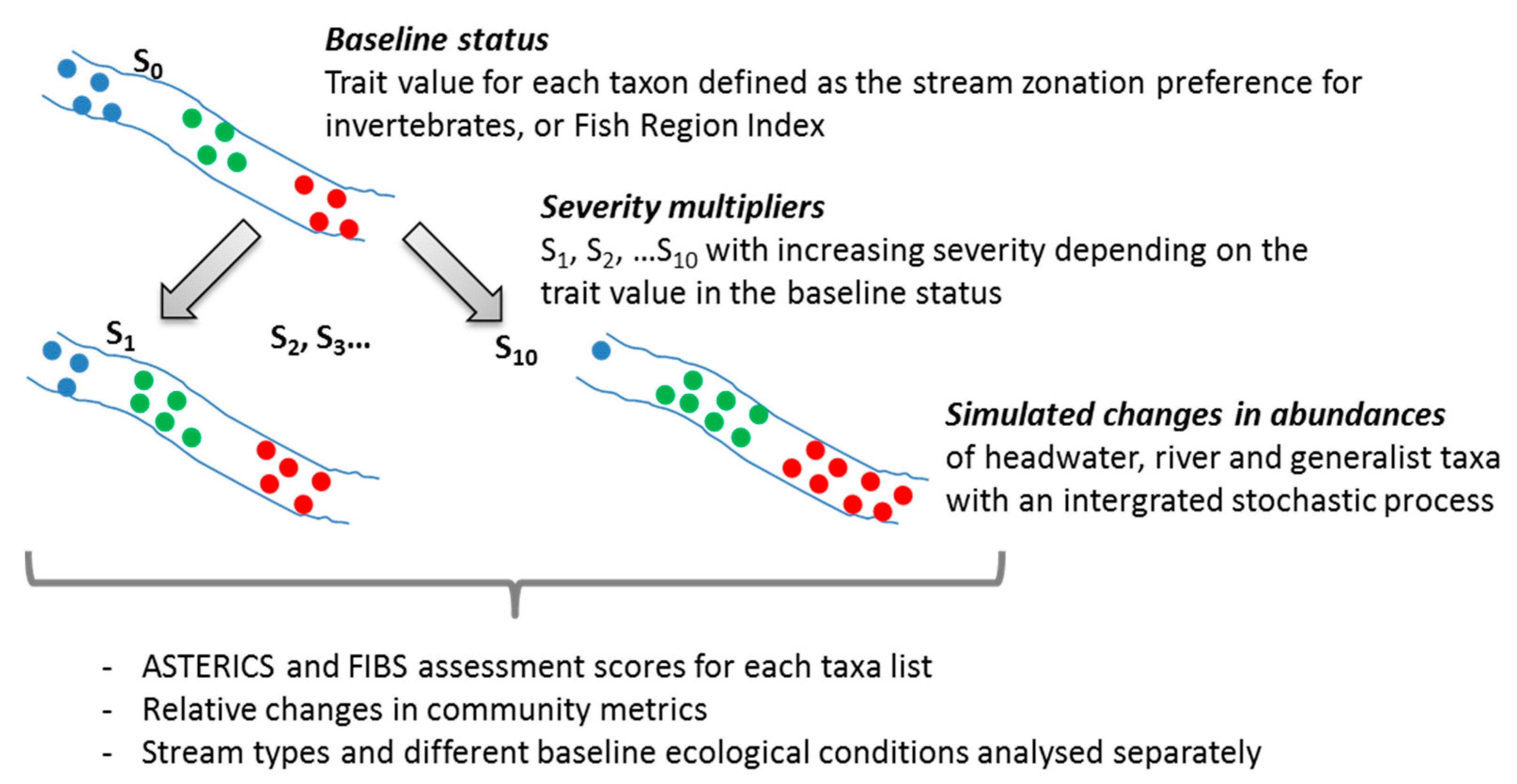
2.2. Multipliers Reflecting Climate Change Effects
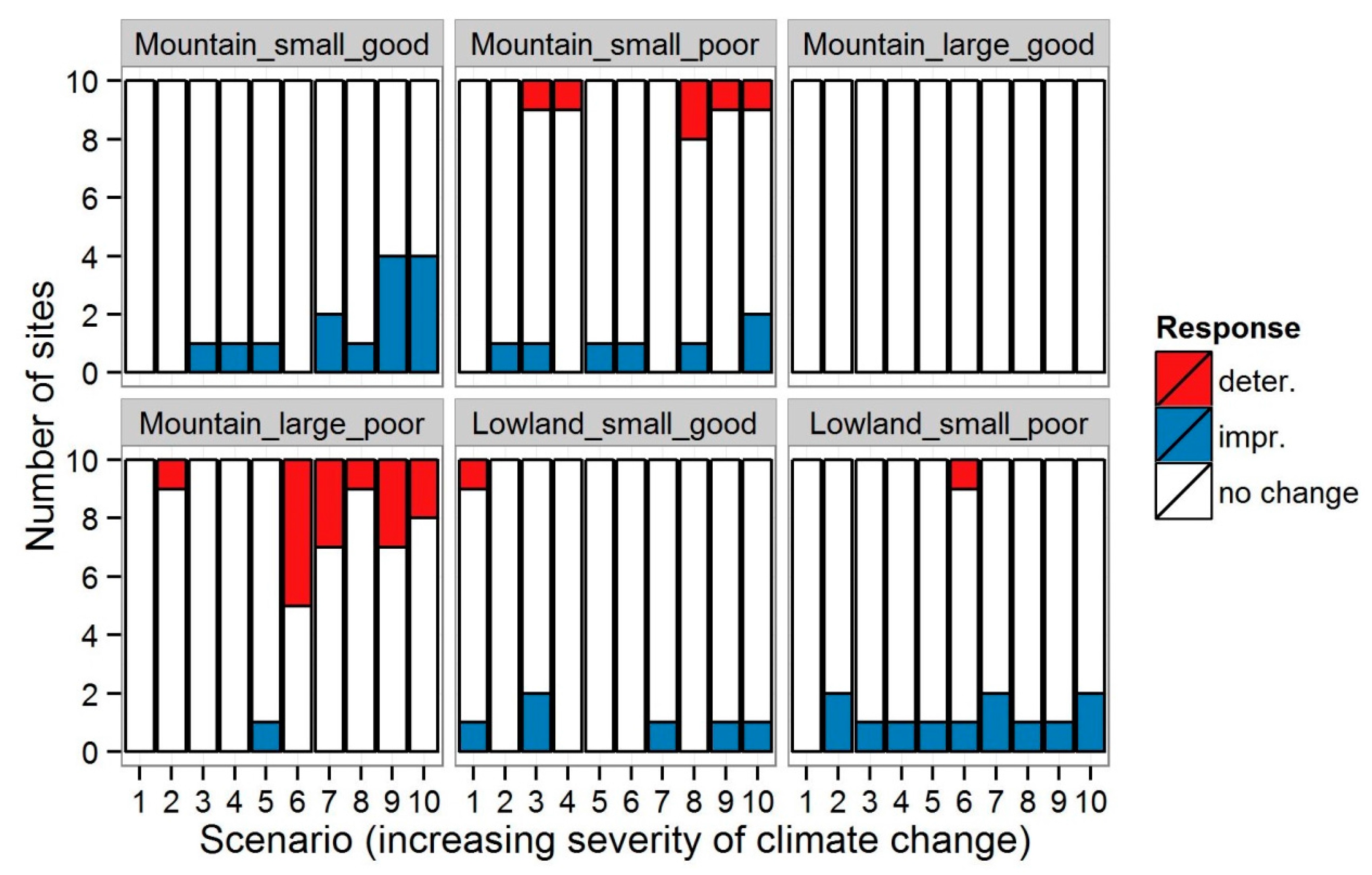
2.3. Metrics and Assessment Results
3. Results
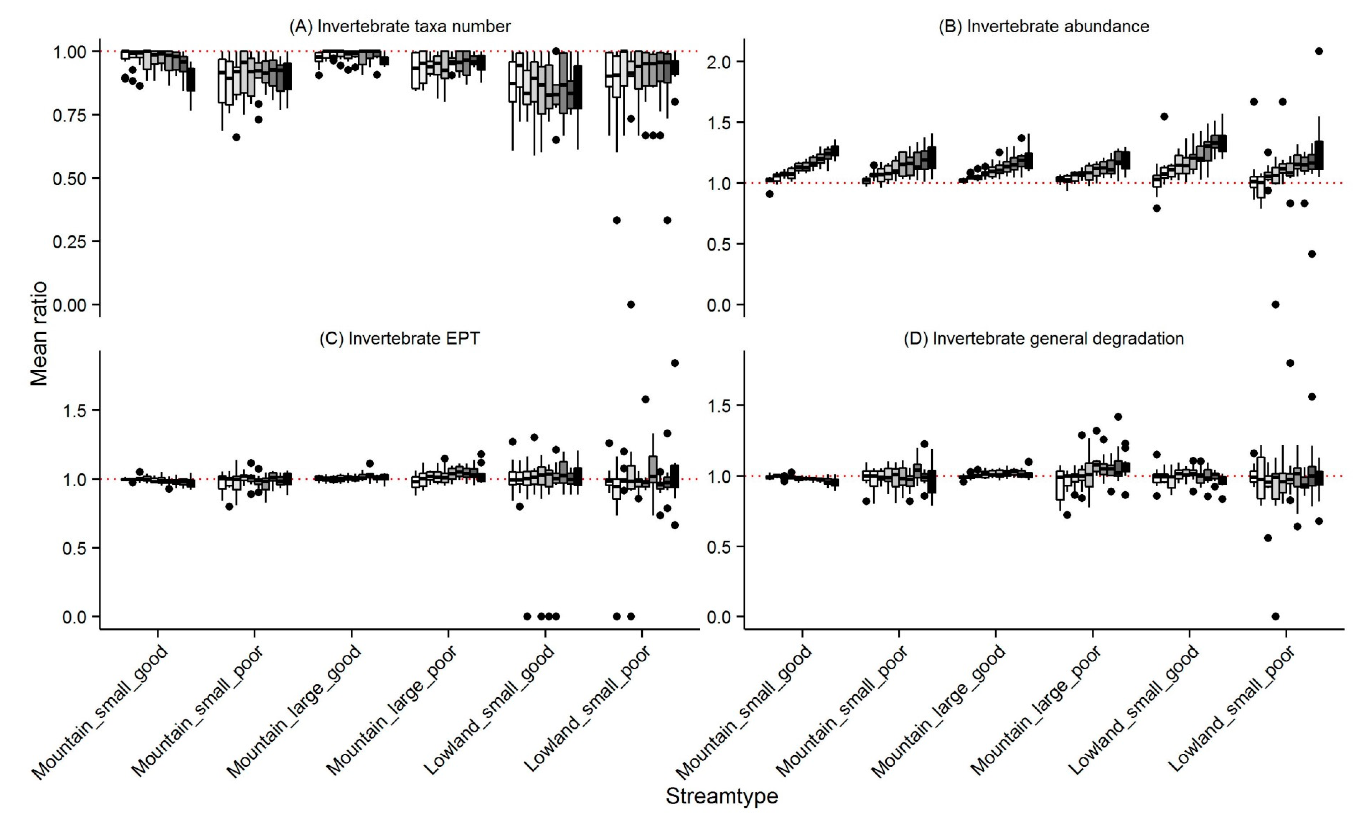
3.1. Invertebrates
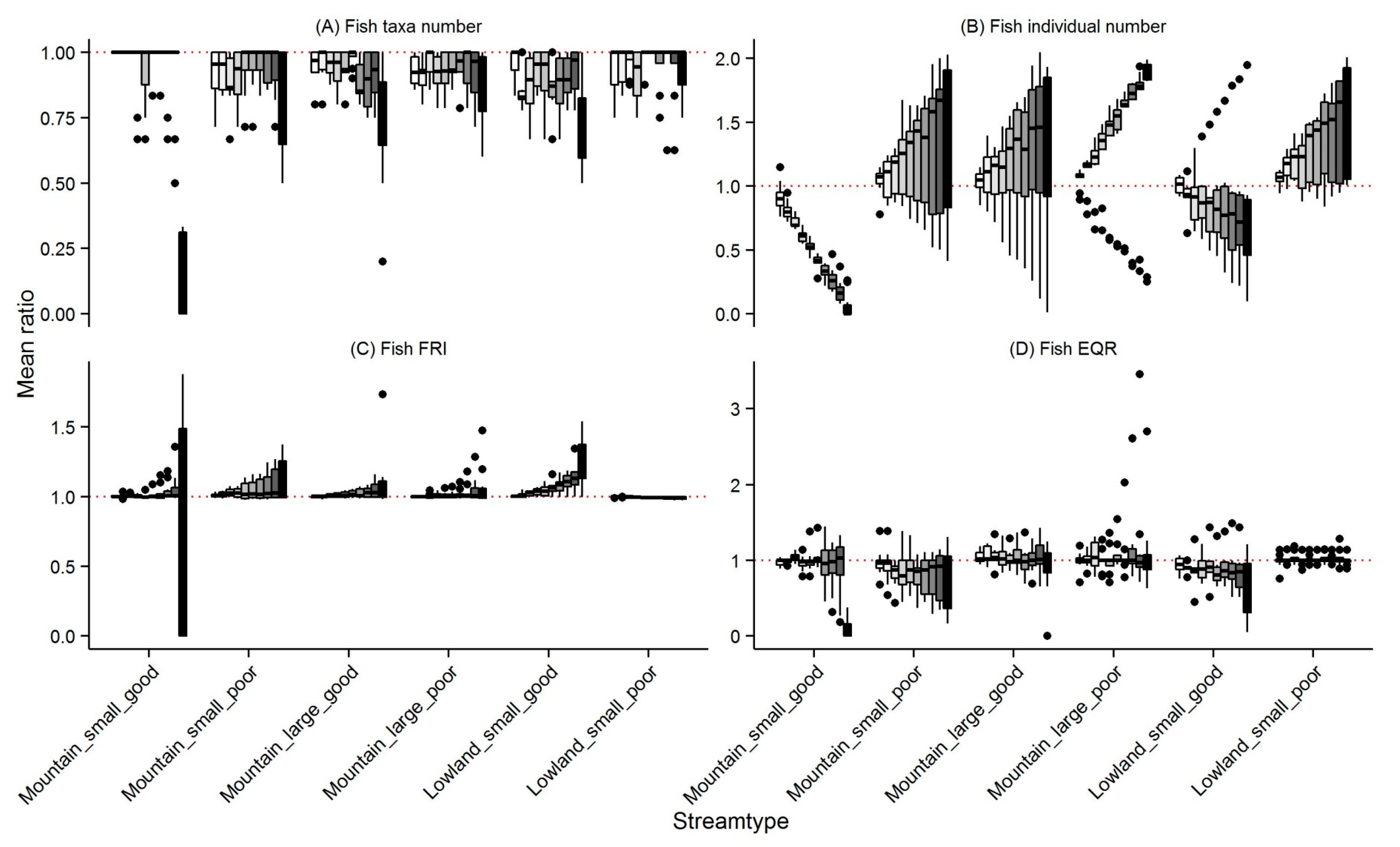
3.2. Fish
4. Discussion
4.1. Changes in Community Metrics
4.2. Directions for Future Analyses
4.3. Climate Change Induced Range Shifts and Implications for Assessment
Supplementary Materials
Acknowledgments
Author Contributions
Conflicts of Interest
Abbreviations
| ASTERICS | AQEM/STAR Ecological River Classification System; the standard assessment software for several European states based on invertebrates |
| BSDA | “Basic Statistics and Data Analysis” package in r, version 1.01 |
| EPT | Ephemeroptera, Plecoptera, Trichoptera |
| EQC | Ecological Quality Class |
| EQR | Ecological Quality Ratio |
| FIBS | Fischbasiertes Bewertungssystem, german for: fish-based assessment system; standard assessment software for fish in Germany |
| FRI | Fish Region Index |
| HBI | Hilsenhoff’s biotic index |
| IPCC | Intergovernmental Panel on Climate Change |
| S0 | original taxa list |
| S1–S10 | 10 multiplier scenarios, where higher numbers indicate an increasing climate change effect |
| WFD | Water Framework Directive |
References
- Vörösmarty, C.J.; McIntyre, P.B.; Gessner, M.O.; Dudgeon, D.; Prusevich, A.; Green, P.; Glidden, S.; Bunn, S.E.; Sullivan, C.A.; Liermann, C.R.; et al. Global threats to human water security and river biodiversity. Nature 2010, 467, 555–561. [Google Scholar] [CrossRef] [PubMed]
- Reist, J.D.; Wrona, F.J.; Prowse, T.D.; Power, M.; Dempson, J.B.; Beamish, R.J.; King, J.R.; Carmichael, T.J.; Sawatzky, C.D. General effects of climate change on Arctic fishes and fish populations. Ambio 2006, 35, 370–380. [Google Scholar] [CrossRef]
- Brown, L.E.; Hannah, D.M.; Milner, A.M. Vulnerability of alpine stream biodiversity to shrinking glaciers and snowpacks. Glob. Chang. Biol. 2007, 13, 958–966. [Google Scholar] [CrossRef]
- Domisch, S.; Jähnig, S.C.; Haase, P. Climate-change winners and losers: Stream macroinvertebrates of a submontane region in Central Europe. Freshw. Biol. 2011, 56, 2009–2020. [Google Scholar] [CrossRef]
- Bonada, N.; Doledec, S.; Statzner, B. Taxonomic and biological trait differences of stream macroinvertebrate communities between mediterranean and temperate regions: Implications for future climatic scenarios. Glob. Chang. Biol. 2007, 13, 1658–1671. [Google Scholar] [CrossRef]
- European Commission. Report from the Commission to the European Parliament and the Council on the Implementation of the Water Framework Directive (2000/60/EC) River Basin Management Plans; European Commission: Brussels, Belgium, 2012. [Google Scholar]
- Arle, J.; Mohaupt, V.; Kirst, I. Monitoring of Surface Waters in Germany under the Water Framework Directive—A Review of Approaches, Methods and Results. Water 2016, 8, 217. [Google Scholar] [CrossRef]
- Woodward, G.; Perkins, D.M.; Brown, L.E. Climate change and freshwater ecosystems: Impacts across multiple levels of organization. Philos. Trans. R. Soc. Lond. B Biol. Sci. 2010, 365, 2093–2106. [Google Scholar] [CrossRef] [PubMed]
- Haidekker, A.; Hering, D. Relationship between benthic insects (Ephemeroptera, Plecoptera, Coleoptera, Trichoptera) and temperature in small and medium-sized streams in Germany: A multivariate study. Aquat. Ecol. 2008, 42, 463–481. [Google Scholar] [CrossRef]
- Oliva-Paterna, F.J.; Torralva, M.; Fernández-Delgado, C. Threatened Fishes of the World: Aphanius iberus (Cuvier & Valenciennes, 1846) (Cyprinodontidae). Environ. Biol. Fish. 2006, 75, 307–309. [Google Scholar]
- Floury, M.; Usseglio-Polatera, P.; Ferreol, M.; Delattre, C.; Souchon, Y. Global climate change in large European rivers: Long-term effects on macroinvertebrate communities and potential local confounding factors. Glob. Chang. Biol. 2013, 19, 1085–1099. [Google Scholar] [CrossRef] [PubMed]
- Hamilton, A.T.; Stamp, J.D.; Bierwagen, B.G. Vulnerability of biological metrics and multimetric indices to effects of climate change. J. N. Am. Benthol. Soc. 2010, 29, 1379–1396. [Google Scholar] [CrossRef]
- Lawrence, J.E.; Lunde, K.B.; Mazor, R.D.; Bêche, L.A.; McElravy, E.P.; Resh, V.H. Long-term macroinvertebrate responses to climate change: Implications for biological assessment in mediterranean-climate streams. J. N. Am. Benthol. Soc. 2010, 29, 1424–1440. [Google Scholar] [CrossRef]
- Allan, J.D.; Castillo, M.M. Stream Ecology; Springer: Dordrecht, The Netherlands, 2007. [Google Scholar]
- Illies, J. Versuch einer allgemeinen biozönotischen Gliederung der Fließgewässer. Int. Rev. Gesamten Hydrobiol. Hydrogr. 1961, 46, 205–213. [Google Scholar] [CrossRef]
- Schmidt-Kloiber, A.; Hering, D. www.freshwaterecology.info—An online tool that unifies, standardises and codifies more than 20,000 European freshwater organisms and their ecological preferences. Ecol. Indic. 2015, 53, 271–282. [Google Scholar] [CrossRef]
- Pletterbauer, F.; Melcher, A.H.; Ferreira, T.; Schmutz, S. Impact of climate change on the structure of fish assemblages in European rivers. Hydrobiologia 2015, 744, 235–254. [Google Scholar]
- Graham, C.T.; Harrod, C. Implications of climate change for the fishes of the British Isles. J. Fish Biol. 2009, 74, 1143–1205. [Google Scholar] [CrossRef] [PubMed]
- Buisson, L.; Grenouillet, G. Contrasted impacts of climate change on stream fish assemblages along an environmental gradient. Divers. Distrib. 2009, 15, 613–626. [Google Scholar] [CrossRef]
- Sandin, L.; Schmidt-Kloiber, A.; Svenning, J.; Jeppesen, E.; Friberg, N. A trait based approach to assess climate change sensitivity of freshwater invertebrates across Swedish ecoregions. Curr. Zool. 2014, 60, 221–232. [Google Scholar]
- Domisch, S.; Araújo, M.B.; Bonada, N.; Pauls, S.U.; Jähnig, S.C.; Haase, P. Modelling distribution in European stream macroinvertebrates under future climates. Glob. Chang. Biol. 2013, 19, 752–762. [Google Scholar] [PubMed]
- The Intergovernmental Panel on Climate Change (IPCC). Climate Change 2013: The Physical Science Basis; Stocker, T.F., Qin, D., Plattner, G.-K., Tignor, M., Allen, S.K., Boschung, J., Nauels, A., Xia, Y., Bex, V., Midgley, P.M., Eds.; Contribution of Working Group I to the Fifth Assessment Report of the Intergovernmental Panel on Climate Change; Cambridge University Press: Cambridge, UK; New York, NY, USA, 2013; p. 1535. [Google Scholar]
- Haase, P.; Lohse, S.; Pauls, S.; Schindehütte, K.; Sundermann, A.; Rolauffs, P.; Hering, D. Assessing streams in Germany with benthic invertebrates: Development of a practical standardized protocol for macroinvertebrate sampling and sorting. Limnologica 2004, 34, 349–365. [Google Scholar]
- Hering, D.; Schmidt-Kloiber, A.; Murphy, J.; Lücke, S.; Zamora-Muñoz, C.; López-Rodríguez, M.; Huber, T.; Graf, W. Potential impact of climate change on aquatic insects: A sensitivity analysis for European caddisflies (Trichoptera) based on distribution patterns and ecological preferences. Aquat. Sci. Res. Across Bound. 2009, 71, 3–14. [Google Scholar] [CrossRef]
- Hering, D.; Borja, A.; Carvalho, L.; Feld, C.K. Assessment and recovery of European water bodies: Key messages from the WISER project. Hydrobiologia 2013, 704, 1–9. [Google Scholar] [CrossRef]
- Arnholt, A.T. BSDA: Basic Statistics and Data Analysis R Package Version 1.01. 2012. Available online: https://cran.r-project.org/web/packages/BSDA/index.html (accessed on 23 March 2012).
- R Core Team. R: A Language and Environment for Statistical Computing; R Foundation of Statistical Computing: Vienna, Austria, 2015. [Google Scholar]
- Wilby, R.L.; Orr, H.G.; Hedger, M.; Forrow, D.; Blackmore, M. Risks posed by climate change to the delivery of Water Framework Directive objectives in the UK. Environ. Int. 2006, 32, 1043–1055. [Google Scholar] [CrossRef] [PubMed]
- Schmutz, S.; Matulla, C.; Melcher, A.; Gerersdorfer, T.; Haas, P.; Formayer, H. Beurteilung der Auswirkungen Möglicher Klimaänderungen auf die Fischfauna Anhand Ausgewählter Fließgewässer. Endbericht, im Auftrag des BMLFUW, GZ 54 3895/163-V/4/03; Final Project Report; BMLFUW: Stubenring, Austria, 2004. [Google Scholar]
- Daufresne, M.; Boet, P. Climate change impacts on structure and diversity of fish communities in rivers. Glob. Chang. Biol. 2007, 13, 2467–2478. [Google Scholar] [CrossRef]
- Webb, B.; Walsh, A. Changing UK river temperatures and their impact on fish populations. In Hydrology: Science and Practice for the 21 st Century, Proceedings of the British Hydrological Society International Conference, Imperial College, London, UK, 12–16 July 2004; Webb, B., Acreman Maksimovic, C., Smithers, H., Kirby, C., Eds.; British Hydrological Society: Imperial College, London, UK, 2004; pp. 177–191. [Google Scholar]
- United States Environmental Protectior Agency (USEPA). Implications of Climate Change for Bioassessment Programs and Approaches to Account for Effects; EPA/600/R-11/036A; Global Change Research Program, National Center for Environmental Assessment: Washington, DC, USA, 2012.
- Hershkovitz, Y.; Dahm, V.; Lorenz, A.W.; Hering, D. A multi-trait approach for the identification and protection of European freshwater species that are potentially vulnerable to the impacts of climate change. Ecol. Indic. 2015, 50, 150–160. [Google Scholar] [CrossRef]
- Logez, M.; Pont, D. Global warming and potential shift in reference conditions: The case of functional fish-based metrics. Hydrobiologia 2012, 704, 417–436. [Google Scholar] [CrossRef]
- Scheffer, M.; Carpenter, S.; Foley, J.A.; Folke, C.; Walker, B. Catastrophic shifts in ecosystems. Nature 2001, 413, 591–596. [Google Scholar] [CrossRef] [PubMed]
- Hering, D.; Carvalho, L.; Argillier, C.; Beklioglu, M.; Borja, A.; Cardoso, A.C.; Duel, H.; Ferreira, T.; Globevnik, L.; Hanganu, J.; et al. Managing aquatic ecosystems and water resources under multiple stress—An introduction to the MARS project. Sci. Total Environ. 2015, 503–504, 10–21. [Google Scholar] [CrossRef] [PubMed]
- Kuemmerlen, M.; Schmalz, B.; Cai, Q.; Haase, P.; Fohrer, N.; Jähnig, S.C. An attack on two fronts: How predicted climate and land use changes affect the predicted distribution of stream macroinvertebrates. Freshw. Biol. 2015, 60, 1443–1458. [Google Scholar] [CrossRef]
- Hamilton, A.T.; Barbour, M.T.; Bierwagen, B.G. Implications of global change for the maintenance of water quality and ecological integrity in the context of current water laws and environmental policies. Hydrobiologia 2010, 657, 263–278. [Google Scholar]
- Bhowmik, A.K.; Schäfer, R.B. Large Scale Relationship between Aquatic Insect Traits and Climate. PLoS ONE 2015, 10, e0130025. [Google Scholar]
- Lytle, D.A.; Poff, N.L. Adaptation to natural flow regimes. Trends Ecol. Evol. 2004, 19, 94–100. [Google Scholar] [CrossRef] [PubMed]
- Poff, N.L.; Pyne, M.I.; Bledsoe, B.P.; Cuhaciyan, C.C.; Carlisle, D.M. Developing linkages between species traits and multiscaled environmental variation to explore vulnerability of stream benthic communities to climate change. J. N. Am. Benthol. Soc. 2010, 29, 1441–1458. [Google Scholar] [CrossRef]
- Sundermann, A.; Stoll, S.; Haase, P. River restoration success depends on the species pool of the immediate surroundings. Ecol. Appl. 2011, 21, 1962–1971. [Google Scholar] [CrossRef] [PubMed]
- Tonkin, J.D.; Stoll, S.; Sundermann, A.; Haase, P. Dispersal distance and the pool of taxa, but not barriers, determine the colonisation of restored river reaches by benthic invertebrates. Freshw. Biol. 2014, 59, 1843–1855. [Google Scholar] [CrossRef]
- Früh, D.; Stoll, S.; Haase, P. Physico-chemical variables determining the invasion risk of freshwater habitats by alien mollusks and crustaceans. Ecol. Evol. 2012, 2, 2843–2853. [Google Scholar] [CrossRef] [PubMed]
- Früh, D.; Stoll, S.; Haase, P. Physicochemical and morphological degradation of stream and river habitats increases invasion risk. Biol. Invasions 2012, 14, 2243–2253. [Google Scholar] [CrossRef]
- Li, F.; Sundermann, A.; Stoll, S.; Haase, P. A newly developed dispersal metric indicates the succession of benthic invertebrates in restored rivers. Sci. Total Environ. 2016, 569–570, 1570–1578. [Google Scholar] [CrossRef] [PubMed]
- Vaughan, I.P.; Ormerod, S.J. Large-scale, long-term trends in British river macroinvertebrates. Glob. Chang. Biol. 2012, 18, 2184–2194. [Google Scholar] [CrossRef]
- Haase, P.; Li, F.; Sundermann, A.; Lorenz, A.; Tonkin, J.; Stoll, S. Three-dimensional range shifts in biodiversity driven by recent climate warming. PeerJ PrePrints 2015, 3, e1270. [Google Scholar]
- Cañedo-Argüelles, M.; Boersma, K.S.; Bogan, M.T.; Olden, J.D.; Phillipsen, I.; Schriever, T.A.; Lytle, D.A. Dispersal strength determines meta-community structure in a dendritic riverine network. J. Biogeogr. 2015, 42, 778–790. [Google Scholar] [CrossRef]
- Tonkin, J.D.; Stoll, S.; Jähnig, S.C.; Haase, P. Contrasting metacommunity structure and beta diversity in a river-floodplain system. Oikos 2016, 125, 686–697. [Google Scholar] [CrossRef]
- Isaak, D.J.; Young, M.K.; Luce, C.H.; Hostetler, S.W.; Wenger, S.J.; Peterson, E.E.; Ver Hoef, J.M.; Groce, M.C.; Horan, D.L.; Nagel, D.E. Slow climate velocities of mountain streams portend their role as refugia for cold-water biodiversity. Proc. Natl. Acad. Sci. USA 2016, 113, 4374–4379. [Google Scholar] [CrossRef] [PubMed]
- Geismar, J.; Haase, P.; Nowak, C.; Sauer, J.; Pauls, S.U. Local population genetic structure of the montane caddisfly Drusus discolor is driven by overland dispersal and spatial scaling. Freshw. Biol. 2015, 60, 209–221. [Google Scholar] [CrossRef]
- Jaeger, K.L.; Olden, J.D.; Pelland, N.A. Climate change poised to threaten hydrologic connectivity and endemic fishes in dryland streams. Proc. Natl. Acad. Sci. USA 2014, 111, 13894–13899. [Google Scholar] [CrossRef] [PubMed]
- Waters, J.M.; Craw, D.; Burridge, C.P.; Kennedy, M.; King, T.M.; Wallis, G.P. Within-river genetic connectivity patterns reflect contrasting geomorphology. J. Biogeogr. 2015, 42, 2452–2460. [Google Scholar] [CrossRef]
- Altermatt, F.; Seymour, M.; Martinez, N. River network properties shape α-diversity and community similarity patterns of aquatic insect communities across major drainage basins. J. Biogeogr. 2013, 40, 2249–2260. [Google Scholar] [CrossRef]
- Heino, J. The importance of metacommunity ecology for environmental assessment research in the freshwater realm. Biol. Rev. 2013, 88, 166–178. [Google Scholar] [CrossRef] [PubMed]
- Hering, D.; Borja, A.; Carstensen, J.; Carvalho, L.; Elliott, M.; Feld, C.K.; Heiskanen, A.-S.; Johnson, R.K.; Moe, J.; Pont, D.; et al. The European Water Framework Directive at the age of 10: A critical review of the achievements with recommendations for the future. Sci. Total Environ. 2010, 408, 4007–4019. [Google Scholar] [CrossRef] [PubMed]
- Haase, P.; Frenzel, M.; Klotz, S.; Musche, M.; Stoll, S. The long-term ecological research (LTER) network: Relevance, current status, future perspective and examples from marine, freshwater and terrestrial long-term observation. Ecol. Indic. 2016, 65, 1–3. [Google Scholar] [CrossRef]
- Halle, M.; Müller, A.; Sundermann, A. Temperature Preferences of Benthic Invertebrates as a Basis to Indicate Climate Change Effects in Rivers on the Biocenosis (in German: Ableitung von Temperaturpräferenzen des Makrozoobenthos für die Entwicklung eines Verfahrens zur Indikation Biozönotischer Wirkungen des Klimawandels in Fließgewässern); KLIWA-Berichte Heft 20; LUBW Landesanstalt für Umwelt, Messungen und Naturschutz Baden-Württemberg: Karlsruhe, Germany, 2016. [Google Scholar]


| Zone | Eu-Crenal | Hypo-Crenal | Epi-Rhithral | Meta-Rhithral | Hypo-Rhithral | Epi-Potamal | Meta-Potamal | Hypo-Potamal |
|---|---|---|---|---|---|---|---|---|
| Fish zone | Trout zone | Grayling zone | Barbel zone | Bream zone | ||||
| Dominant species | Salmo trutta | Thymallus thymallus | Barbus barbus | Abramis brama | ||||
| Summer temp. °C | <10 | <10 | <15 | >15 | ~20 | |||
| Amplitude < °C | 2 | 5 | 9 | 13 | 18 | 20 | >20 | |
| Fish Region Index (FRI) | 3 | 4 | 5 | 6 | 7 | 8 | ||
| Headwater taxa | FRI ≤ 5.0: Abundance decrease, e.g., Salvelinus fontinalis, FRI = 3.5 | |||||||
| River taxa | 5.0 < FRI ≤ 7.0: Abundance increase, e.g., Barbus barbus, FRI = 6.08 | |||||||
| Estuary taxa | FRI > 7.0 no change, e.g., Gasterosteus aculeatus, FRI = 7.17 | |||||||
| Zone | Eu-Crenal | Hypo-Crenal | Epi-Rhithral | Meta-Rhithral | Hypo-Rhithral | Epi-Potamal | Meta-Potamal | Hypo-Potamal |
|---|---|---|---|---|---|---|---|---|
| Headwater taxa | ∑preferences = 8–10: Abundance decrease | |||||||
| Generalist taxa | ∑preferences = 8–10 AND classification required in all 5 zones *: Abundance increase | |||||||
| River taxa | ∑preferences = 8–10: Abundance increase | |||||||
| Examples | ||||||||
| Odontocerum albicorne (headwater) | 0 | 2 | 7 | 1 | 0 | 0 | 0 | 0 |
| Baetis rhodani (generalist) | 0 | 1 | 2 | 3 | 2 | 1 | 1 | 0 |
| Aphelocheirus aestivalis (river) | 0 | 0 | 0 | 0 | 2 | 8 | 0 | 0 |
| Polycentropus flavomaculatus (no change) | 0 | 0 | 0 | 2 | 2 | 2 | 2 | 2 |
| S1 | S2 | S3 | S4 | S5 | S6 | S7 | S8 | S9 | S10 | ||
|---|---|---|---|---|---|---|---|---|---|---|---|
| Invertebrates | |||||||||||
| Headwater taxa | < | 0.9 | 0.8 | 0.7 | 0.6 | 0.5 | 0.4 | 0.3 | 0.2 | 0.1 | 0.0 |
| Generalist taxa | > | 1.05 | 1.1 | 1.15 | 1.2 | 1.25 | 1.3 | 1.35 | 1.4 | 1.45 | 1.5 |
| River taxa | > | 1.05 | 1.1 | 1.15 | 1.2 | 1.25 | 1.3 | 1.35 | 1.4 | 1.45 | 1.5 |
| n/a | / | 1.0 | 1.0 | 1.0 | 1.0 | 1.0 | 1.0 | 1.0 | 1.0 | 1.0 | 1.0 |
| Fish | |||||||||||
| FRI ≤ 5.0 | < | 0.9 | 0.8 | 0.7 | 0.6 | 0.5 | 0.4 | 0.3 | 0.2 | 0.1 | 0.0 |
| 5.0 < FRI ≤ 7.0 | > | 1.1 | 1.2 | 1.3 | 1.4 | 1.5 | 1.6 | 1.7 | 1.8 | 1.9 | 2 |
| FRI > 7.0 | / | 1.0 | 1.0 | 1.0 | 1.0 | 1.0 | 1.0 | 1.0 | 1.0 | 1.0 | 1.0 |
© 2017 by the authors. Licensee MDPI, Basel, Switzerland. This article is an open access article distributed under the terms and conditions of the Creative Commons Attribution (CC BY) license (http://creativecommons.org/licenses/by/4.0/).
Share and Cite
Jähnig, S.C.; Tonkin, J.D.; Gies, M.; Domisch, S.; Hering, D.; Haase, P. Severity Multipliers as a Methodology to Explore Potential Effects of Climate Change on Stream Bioassessment Programs. Water 2017, 9, 188. https://doi.org/10.3390/w9040188
Jähnig SC, Tonkin JD, Gies M, Domisch S, Hering D, Haase P. Severity Multipliers as a Methodology to Explore Potential Effects of Climate Change on Stream Bioassessment Programs. Water. 2017; 9(4):188. https://doi.org/10.3390/w9040188
Chicago/Turabian StyleJähnig, Sonja C., Jonathan D. Tonkin, Maria Gies, Sami Domisch, Daniel Hering, and Peter Haase. 2017. "Severity Multipliers as a Methodology to Explore Potential Effects of Climate Change on Stream Bioassessment Programs" Water 9, no. 4: 188. https://doi.org/10.3390/w9040188