Study on the Formation and Initial Transport for Non-Homogeneous Debris Flow

Abstract

Non-homogeneous debris flows generally occur during the rainy seasons in Southwest China, and have received considerable attention in the literature. Regarding the complexity in debris flow dynamics, experimental approaches have proven to be effective in revealing the formative mechanism for debris flow, and quantifying the relations between the various influencing factors with debris-flow formation and subsequent transport processes. Therefore, a flume-based and experimental study was performed at the Debris Flow Observation and Research Station of Jiangjia Gully in Yunnan Province, to theoretically analyze favorable conditions for debris-flow formation and initial transport by selecting the median particle size d₅₀, flow rate Q, vertical grading coefficient ψ, slopes S, and the initial soil water contents W as the five variables for investigation. To achieve this, an optimal combination of these variables was made through an orthogonal experimental design to determine their relative importance upon the occurrence and initial mobilization behavior of a debris flow and to further enhance our insight into debris-flow triggering and transport mechanisms.

1. Introduction

Debris flows are some of the most widespread and prevalent hazards in mountainous environments [1]. In China, much of its mountainous terrain, with complex geological environments and variable monsoon climates, is favorable for the occurrence of debris flows during intense rainy seasons and consequently poses a great threat to the safety of human lives and infrastructure. For this reason, the disasters associated with debris-flow events have drawn considerable attention. Accordingly, a detailed understanding of the formative process and initial transport of debris flows is crucial not only for gaining insights into the debris-flow mechanism, but also for predicting and avoiding debris-flow hazards.

It is well-known that debris flows are commonly triggered by a combination of three essential factors: sufficient solid loose materials, ample water supply, and steep terrain [2,3]. At present, however, most of the relevant studies generally concentrate on the occurrence of debris flows in relation with a single or some particular factors. Some authors assume that rainfall is critical for the debris flow initiation. For instance, Giannecchini et al. [4] obtained critical rainfall input thresholds for debris flows that hit the southern Apuan area in Italy with a deterministic approach; Zhuang et al. [5,6] investigated the thresholds between rainfall and volume of debris flow; Hu et al. [7] derived critical rainfall that leads to the debris-flow occurrence. In these studies, the rainfall intensity–duration (ID) that trigger debris flows has been studied the most (e.g., [8,9,10,11]. Likewise, many authors focus on the debris flows induced by runoff, particular for the wildfire-related debris-flow initiation (e.g., [12,13,14]). For example, Cannon et al. [12] observed that a runoff-dominated process of progressive sediment entrainment by surface runoff, rather than infiltration-triggered failure of discrete soil slips, was the primary mechanism of debris-flow initiation from wildfire. Lanza et al. [15] showed that an area–slope relationship for the Martian gullies is consistent with that observed for terrestrial gullies formed by debris flow, and further inferred that the Martian gullies formed as the result of the saturation of near-surface regolith by a liquid. Legg et al. [16] believed that debris flow initiation apparently occurs within proglacial gullies in the presence of, and perhaps in response to, surface runoff. Additionally, some investigators have their interests exclusively focused to the onset of debris flows under the effect of slope gradient (e.g., [17,18]), materials/soils supplied (e.g., [19,20,21,22,23]), or soil mechanics (e.g., [24,25,26,27]).

In contrast, very few studies have been conducted on debris flows initiated by all the possible key factors. Cui [28] proposed that a curved surface in the three dimensional coordinate system (made up by the coordinate axes of bed slope, saturated degree, and fine grain content) can fully reflect the conditions of debris flow initiation. Klubertanz et al. [29] identified possible factors governing debris flow initiation and established a three-phase model. The former study investigated a combined effect of all the key factors on debris-flow occurrence, indicative of a curved surface. The latter one is purely theoretical and obtained some results in contradiction with many statements found in the literature (e.g., a maximum debris displacement was derived at the lowest slope angle). In fact, the causative factors selected to predict the occurrence of debris-flow differ greatly between different research groups [30], and their relative contribution for the occurrence of debris-flow is still unknown. Because the field study involves great difficulty and uncertainty, this study therefore attempts to select some intrinsic parameters to represent the formative conditions (i.e., flow, loose debris, and gradient), and further determine their impacts on the occurrence of debris flows through experimental flume study and statistical analysis. Here, the flow (i.e., clear water) refers to the process from precipitation and infiltration to runoff that is associated with debris-flow initiation and transport. The flow is not only an important contributing factor for the debris-flow formation, but is also viewed as a significant component of debris flows [31].

2. Experimental Design

2.1. Factor Selection

Steep topography, massive loose debris, and intense rainfall/runoff are prerequisites for debris-flow occurrence. In this regard, the influencing factors were selected to reflect these basic criteria as identifiable variables in detail. Therefore, both the median grain size d₅₀ and the way that coarse and fine particles were distributed in the vertical profile were used as a surrogate for debris condition, the flow rate and initial water content (or moisture content) within the debris were adopted as an index of the rainfall/run-off effect, and the steepness of the watershed could be represented by the flume slope. Thus, the five factors and test levels of each factor are shown in

Table 1. Test levels of the five factors that affect debris-flow formation and initial transport.

Factor Level	(A) Median Grain Size d50 (mm)	(B) Flume Slope S (°)	(C) Flow Rate Q a (m3/h)	(D) Initial Water Content W (%)	(E) Vertical Grading coefficient ψ
1	3.0	25	1.0	4	0.43
2	5.0	30	3.0	10	1.00
3	7.0	35	5.0	20	2.33
4			10.0

Note: ^a Flow rate of clear water.

.

The non-homogeneous debris flows are commonly modeled as two-phase flows because both fine and coarse particles play an important role in the composition and dynamic flow process. In a two-phase debris flow model, the fluid phase is composed of water and fine sediments that are less than the critical grain size d₀, with the solid phase consisting of grain sizes larger than d₀. In earlier studies, a constant critical value of d₀ = 2.0 mm [32] was utilized due to the limitations of the rheological instruments. More recently, Shu et al. [33] introduced a minimum energy dissipation modelling approach [34] to determine d₀ for the experimental debris flows in the Jiangjia gully. Their results implied that the critical diameter d₀ could vary for the different types of debris flows, but with a predicted range of 4.0–7.0 mm.

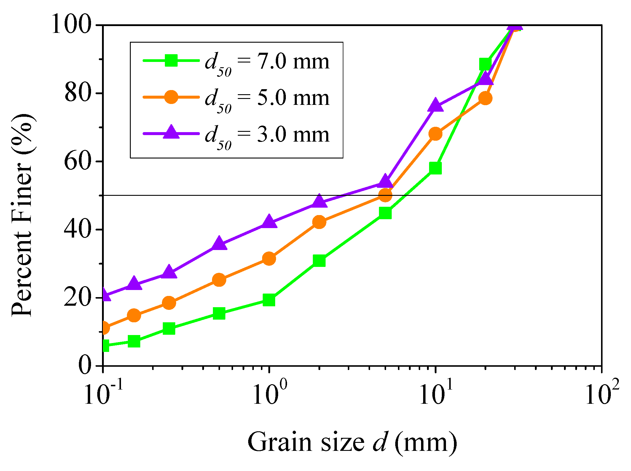
In the case of loose debris collected from the Jiangjiagou valley, the three levels of median grain sizes d₅₀ were determined according to critical grain size d₀ to separate the liquid and solid phases within non-homogeneous debris flows from Shu et al. [33,35], that is, the median grain size d₅₀ is larger, close to, and smaller than the critical grain size d₀ (i.e., ≈4.0–6.0 mm), and hence the cumulative grading curves of experimental debris in the present study are shown in Figure 1. The loose debris was originally from easily-weathered slate, dolomite, and phyllite with a density corresponding to 2.65 t/m³.

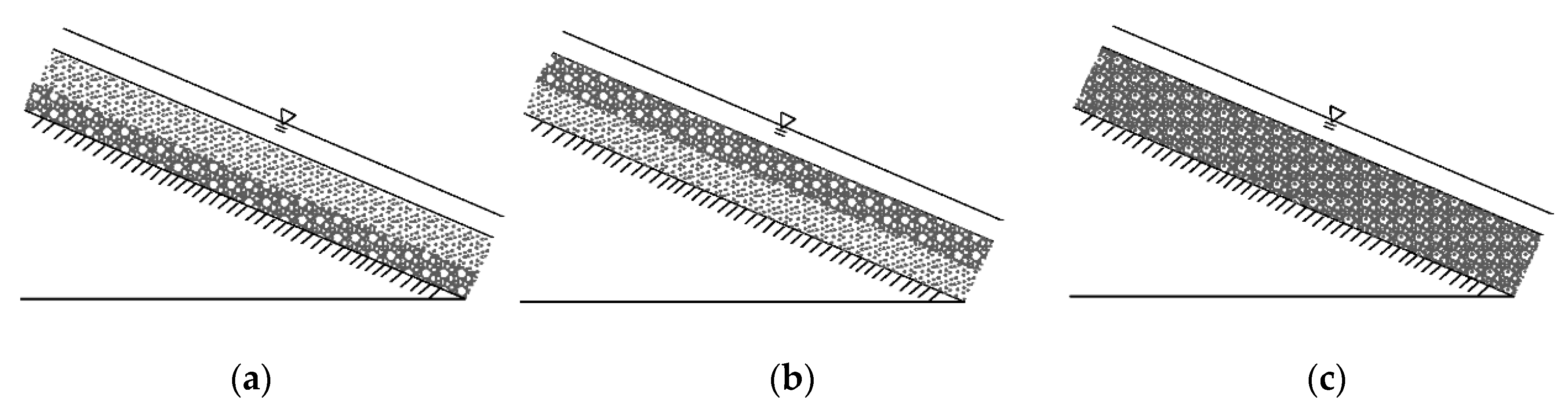
In addition, it is to be emphasized that the way that coarse and fine particles appeared in the vertical profile within loose debris was also considered on the basis of three vertical depositing patterns (i.e., normal, mixed, and inverse grading) reported in the earlier studies [36,37,38,39,40,41]. However, these findings of the vertical grading patterns were generally restricted to the post-event analysis and alluvial deposits. The study of the vertical grading of debris in the initiation zone and their corresponding effects on the debris-flow dynamic process is relatively scarce. Because of this, three typical vertical grading patterns were considered herein and their influence on the debris-flow formation and initial transport will be examined.

Specifically, coarse particles placed at the bottom layer and fine sediment on the top layer (Case E1, see Figure 2a), the coarse particles distributed on the top layer with fine grains at the bottom layer (Case E3, see Figure 2b), and both the coarse and fine particles fully mixed and covering the whole vertical profile (Case E2, see Figure 2c). In order to quantify this, a vertical grading coefficient ψ was proposed and written as

$$\psi =\frac{d_{50-u}}{d_{50-l}}$$

(1)

where d_50-u and d_50-l represents the median grain size of the graded sediment on the top and bottom layer within the bulk debris, respectively. In this study, three basic debris fractions were used to generate a desirable mixture; fine debris with d₅₀ = 3.0 mm, coarse debris with d₅₀ = 7.0 mm, and an intermediate one with d₅₀ = 5.0 mm. Therefore, the vertical grading coefficient for the corresponding debris configurations can be ψ = 0.43 for Case E1 (i.e., fine particles in the top layer and coarse particles at the basal layer, e.g., d_50-u ≈ 3.0 mm, d_50-l ≈ 7.0 mm), and ψ = 2.33 for Case E3 (coarse particles in the top layer and fine particles at the basal layer, e.g., d_50-u ≈ 7.0 mm, d_50-l ≈ 3.0 mm), respectively. As for case E2, the mixture was generated by thoroughly mixing varying-sized particles that were placed uniformly through the vertical profile to produce a more homogeneous vertical grading pattern (i.e., d_50-u ≈ d_50-l ≈ 3.0, 5.0, 7.0 mm), therefore, ψ = 1.00 for Case E2. In contrast, the test levels for the remaining factors (i.e., flow rate, flume slope, and initial water content) were determined by preliminary experiments.

In general, a more straightforward way to examine the influence of various factors is directly achieved through one-factor-at-a-time or mono-variate design, in which most factors in the system are held constant while one factor is focused on and varied to examine its effect [42,43]. However, this design method will lose its advantage if the number of investigated factors is increased. In contrast, the orthogonal experimental design is more desirable (i.e., gaining the desired result by reducing the number of experiments) in the present study when considering the number of factors and their test levels given in Table 1.

2.2. Experimental Setup and Procedure

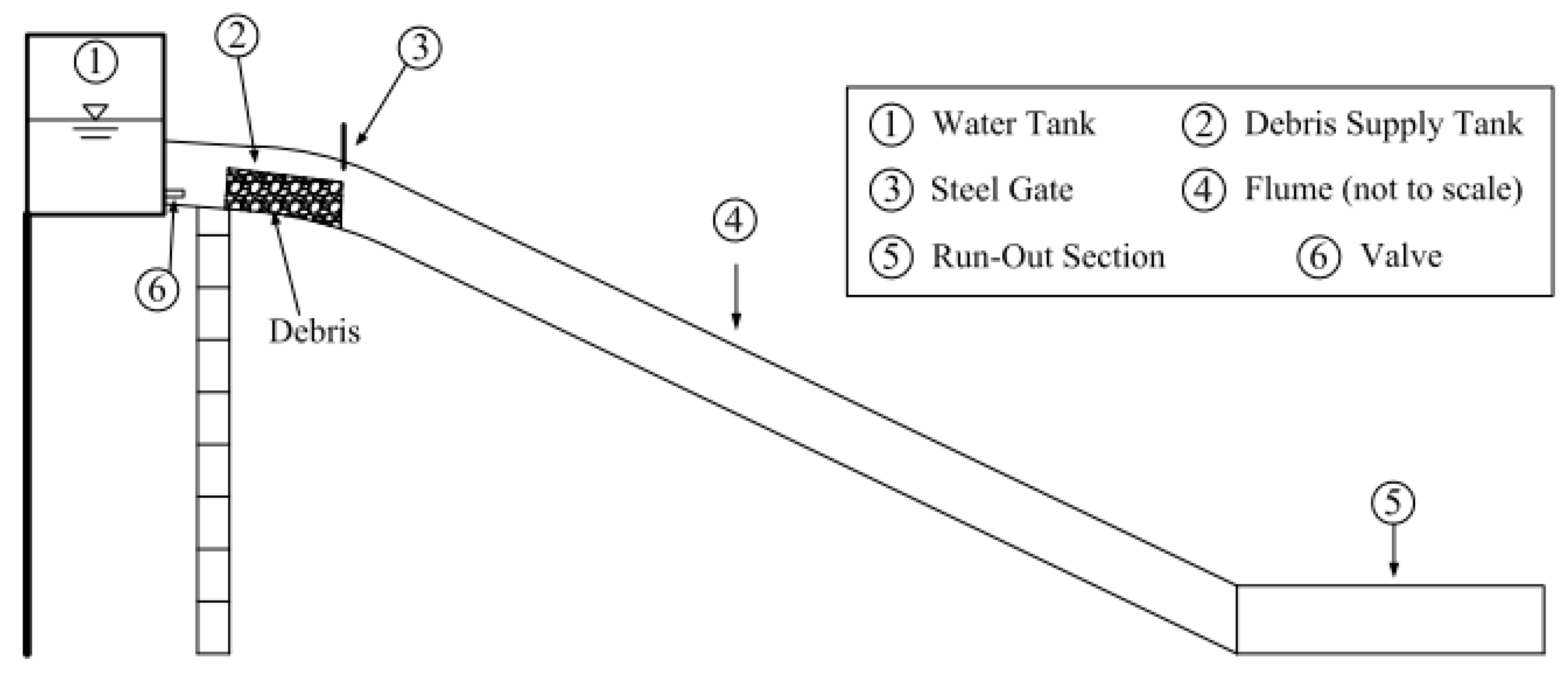
Our experiments were performed in a 9.0 m long, 0.3 m wide, 0.4 m deep flume established in the Debris Flow Observation and Research Station of Jiangjia Gully, the largest field research center in China which is also known as “the debris flow museum” [23]. The facility (Figure 3) consists of a water tank (5.0 m above the laboratory floor which stores water up to 1.2 m³) with a valve at its base (the target flow can be generated by controlling the valve), a mixing supply tank followed by a steel gate, and flume divided into a steep upstream reach (6.0 m long and the chute slope can vary from 25° to 40°) and flat-oriented downstream section (3.0 m long and the flume bed slope can be adjusted from 1° to 5°).

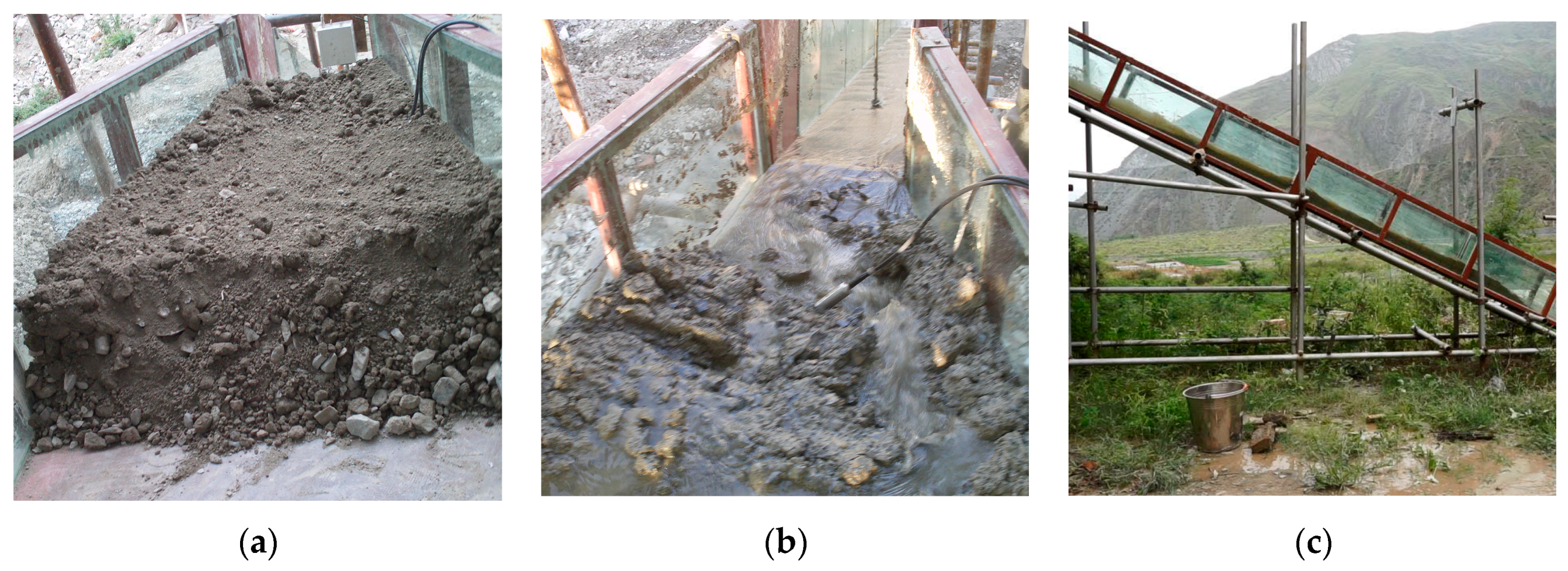
Prior to each run, the debris mixtures were carefully placed in the supply tank (see Figure 3) according to the initial water content (Table 1) and vertical grading coefficient (Table 1 and Figure 2), the volume of solid debris was estimated to be around V_s ≈ 0.10 m³ and remained approximately constant between runs, and then the pore-water pressure sensors (the sensor model is 730-13E-00005 manufactured by a PSI Pressure System company that located at Baytown, TX, USA; the range is a 1.5 m water column; the precision is a 1 mm water column; the operating temperature range is between 0° and 40°) were buried in four locations at 0.3 H, in which H is the height of the debris prior to testing. These sensors are quite small and have a negligible effect on the initial flow formation.

After this, the valve of the water tank was opened to a pre-determined position with the purpose of generating the target flow (i.e., constant flow), and the variability in the flow infiltration level within the mass entity prior to the debris-flow occurrence was accordingly monitored by a video-camera through the transparent wall at one side of the flume (Note: the steel gate was not used in all tests). Initially, the flow was blocked by the debris materials, and when the water level and associated pressure was increased, then a small volume of water flow was found to penetrate through the stable debris materials. For most of the tests, the water flow passed through the debris mass. However, in some tests with high Q, the water flow accumulated so quickly to make it capable of not only going through the granular mass, but also passing over the surface of the granular mass. Colored plastic beads that “floated” on the debris-flow surface were used as tracers to derive the average flow velocity as the flow depths were commonly low (i.e., h = 0.033–0.147 m). When the mass collapsed, entrained, and formed into a debris flow, the valve was closed and the total flow volume that contributed to the formation of the debris flow was calculated. Individual sediment samples collected from the debris-flow deposition were subsequently dried in an oven, weighed, and sieved for further analysis.

2.3. Debris-Flow Formation and Initial Transport

In this study, the debris-flow formation, initiation, and subsequent transport was a continuous mixture-mobilized process. In order to examine the effect of the five factors on the debris-flow formation, the formative duration ΔT_dff (s) of a debris flow observed within the flume was firstly proposed, namely the duration of the debris-flow formation was equivalent to the length of time from the start of experiment to the initiation of the debris-flow mobilization (see Figure 4a,b). Generally, the shorter the formative duration ΔT_dff measured, the more conducive the conditions for the debris-flow formation/initiation were likely to be. Once the valve of the water tank was opened, the experiment was started and timely recorded; while the initiation of debris flow was defined as the point at which the materials were flooded, mixed, and suddenly entered the flume section. As the debris-flow initiation and transport happened almost simultaneously, the initiation was also defined as the time right before or coincided with a sudden mobilization of the debris-flow mixture into the flume. In each test, the volume of clear water and solid materials that were involved in the debris-flow formation could be roughly estimated as $V_{ol}=V_s+V_f=0.10+Q\times \Delta T_{dff}$.

Secondly, the initial transport following the debris-flow initiation is described by the observed surface velocity u and Froude number Fr (see Figure 4c). Here, the debris-flow Froude number can be expressed in terms of debris-flow (average) velocity as

$$F_r=\frac{u}{\sqrt{gh}}$$

(2)

where u is the mean debris-flow velocity (m/s), h is the debris-flow depth (m) measured at 4.0–5.0 m from the flume upstream end, and g is the gravitational acceleration (m/s²). Note that the velocity and Froude number in this study were restricted to the initial transport of debris flows, that is, when the debris-flow mixture entered into the flume and moved towards the downstream end.

3. Results and Analysis

Following the test levels of the five factors and the experimental design, 48 runs were performed in the flume chute. The details about the experimental conditions and results for each test are given in

Table 2. Experimental conditions and results in this study.

Run No.	Factors					Measured a
	d50 (mm)	S (°)	Q (m3/h)	W (%)	ψ	Tdff (s)	u (m/s)	Fr
No. 1	7	25	5	0.10	1.00	73
No. 2	3	25	3	0.04	1.00	199	2.82	4.02
No. 3	7	25	5	0.10	0.43	149	4.38	6.26
No. 4	5	25	10	0.20	1.00	125
No. 5	7	25	5	0.10	2.33	255	2.83	4.05
No. 6	5	25	10	0.20	2.33	150	2.93	4.19
No. 7	7	25	1	0.20	1.00	99
No. 8	3	25	3	0.04	2.33	470	2.56	3.66
No. 9	3	25	3	0.04	0.43	228	2.05	2.93
No. 10	5	25	10	0.20	0.43	139	3.09	4.42
No. 11	7	25	1	0.20	0.43	175	1.72	2.46
No. 12	7	25	1	0.20	2.33	156	1.90	2.72
No. 13	5	30	5	0.10	2.33	169	2.98	4.26
No. 14	5	30	5	0.10	0.43	125	3.08	4.39
No. 15	5	30	5	0.10	1.00	77	3.29	4.70
No. 16	7	30	3	0.20	0.43	108	2.50	3.57
No. 17	7	30	3	0.20	2.33	155	2.73	3.90
No. 18	7	30	3	0.20	1.00	124	2.42	3.45
No. 19	7	30	10	0.04	2.33	81	3.18	4.54
No. 20	7	30	10	0.04	1.00	143	3.40	4.86
No. 21	7	30	10	0.04	0.43	218	3.32	4.75
No. 22	3	30	1	0.20	0.43	112	2.75	3.92
No. 23	3	35	5	0.20	0.43	116	2.87	4.10
No. 24	3	35	5	0.20	2.33	105	2.53	3.62
No. 25	3	35	5	0.20	1.00	75	2.66	3.80
No. 26	7	35	5	0.04	0.43	117	2.88	4.11
No. 27	7	35	3	0.10	1.00	77	2.83	4.04
No. 28	7	35	3	0.10	0.43	97	3.17	4.53
No. 29	7	35	3	0.10	2.33	100	2.73	3.89
No. 30	5	35	3	0.20	2.33	86	3.30	4.71
No. 31	5	35	3	0.20	0.43	80	2.80	3.99
No. 32	5	35	3	0.20	1.00	120	2.41	3.45
No. 33	5	35	1	0.04	0.43	1	2.80	3.99
No. 34	7	35	1	0.10	0.43	72	3.29	4.69
No. 35	7	35	10	0.20	0.43	98	3.96	5.66
No. 36	3	35	10	0.10	2.33	145	3.53	5.04
No. 37	3	35	10	0.10	0.43	133	3.58	5.12
No. 38	3	35	10	0.10	1.00	92	3.67	5.24
No. 39	7	35	5	0.04	2.33	170	3.47	4.95
No. 40	7	35	5	0.04	1.00	214	2.94	4.19
No. 41	7	35	10	0.20	1.00	122	2.85	4.08
No. 42	7	35	10	0.20	2.33	105	3.28	4.69
No. 43	7	30	1	0.20	1.00	68	2.10	2.25
No. 44	7	30	3	0.20	2.33	73	2.70	3.72
No. 45	7	30	3	0.20	2.33	73	2.70	2.25
No. 46	7	30	1	0.20	1.00	68	2.10	3.72
No. 47	5	35	1	0.04	0.43	35	2.00	2.04
No. 48	5	35	1	0.04	1.00	50	1.90	1.84

Note: ^a total volume V_ol of the debris flow was obtained by summing the water and debris volume, respectively. The mean and standard deviation of the volume are statistically estimated to be V_ol = 0.277 ± 0.14 m³.

. It is noted that the initial debris-flow velocity has not been measured in some tests. The debris-flow formative duration ΔT_dff is shown to vary between 1.0 and 470 s, and the initial velocity u ranged between 1.72 and 4.38 m/s, with corresponding Fr values generally greater than unity, indicative of a super-critical flow regime. Also, a statistical analysis showed that the sum of water-and-debris volume that leads to debris flows in our experiments averaged V_ol = 0.277 m³ with a standard deviation of 0.14 m³.

Any statistical analysis method has its merits and deficiencies. Therefore, in order to fully and comparatively investigate the relative effect of the five factors on debris-flow initiation, three statistical analytical methods were considered in our study, namely Range analysis (RA), analysis of variance (ANOVA), and Regression analysis. These analyses helped to identify and to obtain a better understanding of the triggering conditions of the debris flow than the study could have obtained by any single investigative approach [44,45].

3.1. Results from the Range Analysis (RA)

Range analysis (RA) is commonly used for orthogonal design studies (Su and Chen, 2015). Here the range analysis was carried out for our experimental results including (i) the duration of debris-flow formation ΔT_dff; (ii) the debris-flow velocity u; and (iii) the debris-flow Froude number Fr, respectively.

Table 3. Impacts of the five parameters on debris-flow formative duration, velocity, and Froude number from the range analysis.

Influenced Parameters	Range Analysis	Influencing Factors
		A (d50)	B (S)	C (Q)	D (W)	E (ψ)
Tdff	k1	96.42	184.83	187.60	160.50	107.88
	k2	122.69	113.86	142.14	120.31	117.82
	k3	167.50	100.45	137.08	110.09	152.87
	k4			129.25
	R	71.08	84.38	58.35	50.41	44.99
u	k1	2.20	2.02	2.06	2.78	2.95
	k2	2.55	2.80	2.69	3.03	2.21
	k3	2.67	2.97	2.82	2.45	2.89
	k4			3.07
	R	0.47	0.95	1.01	0.58	0.74
Fr	k1	3.15	2.89	2.76	3.62	4.17
	k2	3.50	3.88	4.04	4.32	4.01
	k3	3.75	4.17	3.72	4.32	3.10
	k4			4.38
	R	0.60	1.28	1.62	0.70	1.07

presents the results obtained from the range analysis through the orthogonal design method. In Table 3, k1–k3 (or k4) reflects the effect of a particular factor (e.g., factor A) while the other factors are held constant (e.g., factors B–D), and the difference between the maximum and minimum k value of an interested factor (e.g., factor A) is this investigated factor’s range R. Generally, the factor would exert a stronger influence on the formative duration ΔT_dff, velocity u, and Froude number Fr of the non-homogeneous debris flows when R is larger, and the maximum R value corresponds to the dominant factor.

As far as the time elapsed in the formation of non-homogeneous debris flows is concerned, we expect the formative duration ΔT_dff to be as short as possible. Hence, the minimum value among k1, k2, and k3 (and/or k4) corresponds to the optimal level, which is clearly indicated by the lowest level of each curve associated with the influencing factors given in Table 3. A comparison of the R values in Table 3 gives the result as R(B) > R(A) > R(C) > R(D) > R(E). Also, it reveals that the optimal levels were A1 (i.e., d₅₀ = 3.0 mm), B3 (i.e., S = 35°), C4 (i.e., Q = 10.0 m³/h), D3 (i.e., W = 20%), and E1 (i.e., ψ = 0.43), respectively, and shows the relative importance of the five variables.

In contrast to the formative duration ΔT_dff, the influence of the five factors on debris-flow velocity u has a large difference. As mentioned before, the velocity u is mainly confined to the initial transport after the debris-flow formed, and the flow rate Q and slope S exerted greater influence on debris-flow velocity u with R ≈ 1.0 (see Table 3). This is reasonable because the flow rate was the source of momentum and the high flume slope further accelerated the conversion from potential energy to momentum for the debris-flow transport, particular for its initial mobilization. In contrast, the remaining factors (i.e., d₅₀, W, and ψ) have less effect on the debris-flow velocity u with R < 1.0. It is inferred from the experiment that the friction between particles tends to reduce as the initial water content W increases [46], which easily leads to the slide of debris downstream, while the vertical grading configurations potentially caused impacts on the multi-sized particle’s collision, and ultimately exerted influence on the debris-flow initial velocity. In contrast, the median grain size d₅₀ was shown to have a minor effect on the debris-flow initial transport, which is likely to be attributed to an insignificant difference in the d₅₀ values that were taken into account in this study (i.e., 3.0, 5.0, and 7.0 mm).

Both velocity and Froude number were used to describe the initial debris-flow motion. The influence of these five factors (i.e., Q, S, d₅₀, W, and ψ) on the debris-flow Froude number was similar to that found on the debris-flow velocity, as the Froude number is the function of the square of debris-flow velocity. Therefore, the influence of each factor on the debris-flow Froude number was further enhanced if compared with their influence on the corresponding debris-flow velocity, which is clearly indicated by the R values given in Table 3. Again, the influence of the five factors on the debris-flow Froude number can be listed in the following order: flow rate Q > flume slope S > vertical grading coefficient ψ > initial water content W > median grain size d₅₀.

3.2. Results from Analysis of Variance (ANOVA)

It is well-known that random errors are unavoidable and closely associated with any experiments performed manually, even with all variables under exactly the same experimental conditions. This implies that the difference in the collected data might arise not only from various conditions, but also potentially from the experimental errors. Unfortunately, the source of errors is unclear by means of the Range Analysis. As such, analysis of variance (ANOVA) was also performed to identify whether the errors mainly resulted from the variables or experimental operation, which will enable a better understanding of the impact on the results from the influencing factors and reduce any errors being introduced in the analysis [47,48,49,50,51]. In essence, the ANOVA can be useful to determine the influence of any given input parameter and interaction effects by an F-test that decomposes the error sum of squares, in which the degrees of freedom (DF) indicates the number of independent elements in the sum of squares, SS (Factor), which is the deviation of the estimated factor level mean around the overall mean, and the F value shows the significance of the factors’ influence on the results (that is, the factor would have greater influence when the F value is higher). Here the interaction between different factors is ignored and the parameter of significance standard α includes 0.01, 0.05, and 0.10, respectively.

Table 4. Impacts of the five parameters on debris-flow formative duration, velocity, and Froude number from analysis of variance (ANOVA).

Influenced Parameters	Factors	SS	DF	Variance	F b	α
Tdff	Model	893,234.32	12	74,436.19
	A (d50)	18,166.85	2	9083.42	3.86	**
	B (S)	22,888.56	2	11,444.28	4.87	**
	C (Q)	16,765.42	3	5588.47	2.32	*
	D (W)	23,059.56	2	11,529.78	4.90	**
	E (ψ)	28,237.60	2	14,118.80	6.00	***
	Error	84,642.84	36	2351.19 (2404.63 a)
	Total	977,877.16	48
u	Model	378.51	12	31.54
	A (d50)	0.12	2	0.06	0.58
	B (S)	1.51	2	0.75	7.14	***
	C (Q)	5.09	3	1.70	15.71	***
	D (W)	0.68	2	0.34	3.21	**
	E (ψ)	1.34	2	0.67	6.35	***
	Error	3.49	33	0.106 (0.108 a)
	Total	382.00	45
Fr	Model	749.13	12	62.43
	A (d50)	1.76	2	0.88	2.65	**
	B (S)	6.87	2	3.44	10.33	***
	C (Q)	13.70	3	4.57	13.42	***
	D (W)	1.38	2	0.69	2.07
	E (ψ)	3.29	2	1.65	4.94	**
	Error	10.98	33	0.333 (0.340 a)
	Total	760.11	45

Notes: SS = Sum of squares; DF = Degree of freedom; Variance = SS/DF; F is the ratio of a particular factor’s variance to the corresponding error variance (e.g., For factor d₅₀ in a formative ΔT_dff case, F = 9083.42/2351.19); Significance levels: * significant at α = 0.1; ** significant at α = 0.05; and *** significant at α = 0.01, ^a indicates that the experimental error corresponds to the flow rate as Q in the four test levels.

further illustrates the results from the analysis of variance (ANOVA). It is shown that the variance of the most influencing factors is larger than the error mean square (i.e., variance of the error) associated with the debris-flow ΔT_dff, velocity u, and Froude number Fr. This suggests that the variables significantly affect the measured ΔT_dff, u, and Fr.

According to the F values given in Table 4, it is evident that the significance of these five factors for the formative duration ΔT_dff is vertical grading coefficient ψ > initial water content W > flume slope S > median grain size d₅₀ > flow rate Q, for the debris-flow u is flow rate Q > flume slope S > vertical grading coefficient ψ > initial water content W > median grain size d₅₀, and for the Froude number Fr is flow rate Q > flume slope S > vertical grading coefficient ψ > median grain size d₅₀. This is, to some extent, consistent with the simulations made by Klubertanz et al. [29], who claimed that the slope is less important than water-dependent quantities on the debris-flow initiation.

3.3. Results from Regression Analysis

In our study, four experiments are outliers, because the landslides were observed to form and occur rather than debris flows. In order to exclude or reduce the influence of these less-standard tests on the final results, the regression analysis was carried out with a focus on the standard debris-flow tests [47,52].

As five independent variables were considered in this study, the multiple regression method was employed to determine the correlation between a dependent output parameter and the continuous or discrete independent input parameters. In this regard, the correlations between the five influencing variables and the debris-flow ΔT_dff, u, and Fr are determined from the following multiple linear regression equations (i.e., Equations (3)–(5)). Also, the importance of each influence factor is reflected in the standardized coefficients of the proposed functions.

It is obvious that the contribution from the five variables to the formation of the debris-flow duration ΔT_dff can be ordered as: initial water content W > vertical grading coefficient ψ > flume slope S > median grain size d₅₀ > flow rate Q. The effect of initial water content on ΔT_dff is dominant due to the variability of cohesion as mentioned above; the secondary factor is the vertical grading coefficient ψ. In addition, it was found that the initiation of debris flow was not only closely associated with these five variables, but also with other parameters such as the exposure-cum-sheltering factor (Compared with particular-sized sediment in uniform composition, its initiation and transport within a mixture will definitely be influenced by other particles with different sizes. Specifically, the fine particles will be difficult to entrain due to the protection from coarse particles than is observed in uniform sediment configuration; the opposite will be true for coarse particles, as they are more exposed due to the presence of fine particles in graded sediment. This exposure-cum-sheltering effect is typical in a mixture consists of multi-sized sediment, such as in natural debris flows) and internal friction, which warrants further investigation.

As for the measured debris-flow u, the influence of the five factors was ranked as: flow rate Q > flume slope S > vertical grading coefficient ψ > initial water content W > median grain size d₅₀; and for the debris-flow Fr was the initial water content W > flume slope S > flow rate Q > vertical grading coefficient ψ > median grain size d₅₀. Additionally, the larger difference of more than two orders of magnitude among the coefficients of the five factors were shown in Equation (3) rather than in Equations (4) and (5), which implies that some factors tend to have an exceptionally greater impact on the debris-flow formation (e.g., initial water content W, vertical grading coefficient ψ) than on the initial debris-flow transport.

$$\Delta T_{dff}=-0.53Q-7.36S-5.24d_{50}+16.55\psi -327.78W+412.45$$

(3)

$$u=0.47Q+0.22S+0.1d_{50}-0.18\psi -0.14W+0.01$$

(4)

$$F_r=0.08Q+0.135S+0.024d_{50}+0.079\psi -4.072W-0.302$$

(5)

4. Discussion

4.1. Comparison between the Results from the Three Analysis Methods

Table 5. Summary of the results obtained from the range, variance, and regression analysis.

Parameters	Rank	Range Analysis		ANOVA		Regression
Tdff	1	B (S)		E (ψ)	≈	D (W)
	2	A (d50)		D (W)		E (ψ)
	3	C (Q)		B (S)		B (S)
	4	D (W)		A (d50)		A (d50)
	5	E (ψ)		C (Q)		C (Q)
u	1	C (Q)	=	C (Q)	=	C (Q)
	2	B (S)		B (S)		B (S)
	3	E (ψ)		E (ψ)		E (ψ)
	4	D (W)		D (W)		D (W)
	5	A (d50)		A (d50)		A (d50)
		=		=
Fr	1	C (Q)	≈	C (Q)		D (W)
	2	B (S)		B (S)		B (S)
	3	E (ψ)		E (ψ)		C (Q)
	4	D (W)		A (d50)		E (ψ)
	5	A (d50)		D (W)		A (d50)

presents the ranked list of the influence of the five variables obtained from the range analysis, variance analysis, and regression analysis, respectively, on the debris-flow ΔT_dff, u, and Fr. Range analysis is commonly applied to all differences, and the corresponding results involved not only the errors from the variability in the variables, but also from the experimental operations, particular for our experiment that was manually conducted in a tilting flume. Therefore, the results from the range analysis can serve as a reference. In contrast, analysis of variance is one of statistical regression methods that is based on normal distribution; and a main reason for adopting variance analysis in this study was to determine the source of errors and their relevant impact on the final results. Furthermore, the regression analysis is performed to exclude the influence of non-debris-flow tests. In a general sense, it is difficult to determine the results from the different methods that are more accurate. However, the results from the regression model have more practical implications in comparison, as some landslide tests are subtracted from analysis. In this regard, the flow rate Q has the highest impact on the debris-flow velocity u and the initial water content W has the highest impact on the debris-flow ΔT_dff and Fr. However, a closer examination indicates that the ranked list from ANOVA seems to be more close to that from both the Range and Regression analysis as (i) a lateral comparison made among the results for each influenced factor (i.e., ΔT_dff, u, and Fr); and (ii) a longitudinal comparison between the results for both u and Fr obtained from the same analysis approach. In this respect, the ANOVA seems to be more reliable in assessing the relative contribution of the five factors to the debris-flow initiation (see Table 5).

It is also found that the median grain size d₅₀ appeared to have the least impact on the measured ΔT_dff, u, and Fr, which is potentially due to the moderate variations in d₅₀ values adopted in our study. As for the effect of slope on ΔT_dff, u, and Fr, the slope S demonstrates a greater impact on the u and Fr among five factors than on ΔT_dff, according to the ANOVA and regression analyses. This is reasonable as the S values were slopes of the flume (and were achieved by adjusting the flume chute), the formation of debris flows were partially influenced by varying the flume slopes (i.e., 25° → 35°) as a portion of debris was placed in the connection between the supply tank and flume inlet (and the remainder in the supply tank was inclined at a fixed slope of 7°, see Figure 3 and Figure 4).

In addition, the vertical grading coefficient ψ has been shown to influence the debris-flow ΔT_dff dramatically both in the ANOVA and regression analyses. It is implied from previous studies (e.g., [53,54,55] that the vertical emplacement of the debris, particular the fine particles (i.e., silt and clay), tended to affect the ability of retaining water in the unsaturated mass and then influenced the variability in the pore-water pressure, which finally determined the time elapsed in the debris-flow formation.

4.2. Relevance and Implications

It should be noted that the flume-based debris flows in this study can essentially be classified into the gully-type rather than those mobilized from landslide [56]. Again, the similarities (e.g., initial, boundary, geometrical conditions, etc.) between the experimental debris flows with natural flow events were significant for extending the applicability of the relevant findings from the flume-based studies. Here, the Froude number Fr was considered as the basis for judging the similarity issue in the present study (

Table 6. Flow regimes for typical debris flows measured in West China.

Site	Total Number of Debris Flows	Averaged Fr	Supercritical (Fr > 1)		Subcritical (Fr < 1)
			No.	Percent	No.	Percent
This Study (Yunnan)	48	2.39	48	100.0%	0	0
Jiangjia Gully (Yunnan, Kang et al. [61])	18	2.41	18	100.0%	0	0
Jiaba Gully (Sichuan, Jiang et al. [62])	3	1.45	3	100.0%	0	0
ZhouQu–Sanyanyu Gully (Gansu, Deng et al. [63])	3	0.80	1	33.3%	2	66.7%

). It is seen from Table 6 that the Froude number Fr of the experimental debris flows was universally larger than unity, which is similar to the natural debris flows observed in the mountainous areas of Southwest China, indicating that the formation of supercritical flows was associated with debris-flow transport behaviour. Therefore, our study has strong implications for investigating the characteristics of natural debris flows.

It is to be emphasized that the comparison of the Froude number between our experimental flows and natural debris flows observed in Southwest China was made with the aim of identifying the flow regime associated with debris flows that occurred in various locations, and to further apply our experimental results to similar geological and geomorphological settings. Secondly, the initial transport velocity in our study is restricted to the measurements in the debris-flow initiation zone, and is basically different from the debris-flow velocities reported in earlier studies (e.g., [57,58,59,60]), which were measured when debris flows passed through the observation section in the transportation zone. Therefore, it is not advisable to apply the modified Manning equation to predict the initial debris-flow velocities in this study and compare with the general debris-flow transport velocities given in previous studies.

5. Conclusions

According to the pre-existing studies, the five representative factors affecting the formation and initial transport of debris flows were carefully selected for subsequent experimental design, which included the median grain size d₅₀, vertical grading coefficient ψ, flume slope S, flow rate Q, and initial water content W. The median grain size d₅₀ was close to the critical diameter between the liquid and solid phases reported for non-homogeneous debris flows in the Jiangjia Gully, and the vertical grading coefficient ψ represented the typical non-homogeneous distribution of coarse and fine grains in the vertical profile within the supplied materials. The initiation of debris flow was quantified in terms of the formative duration ΔT_dff, whereas the initial transport of the debris flow was given by the velocity u and Froude number Fr.

The contribution of the five variables to the formation and initial transport of debris flows has been determined with three analytical methods (i.e., range analysis, variance analysis, and regression analysis) in this study. According to the merits and limitations associated with each analysis method, the results from the regression analysis have more practical implications. However, the rank listed from ANOVA seems to be more reliable. Consequently, the ranked list that the five variables contributed to the debris-flow u and Fr from this analysis is given as: flow rate Q > flume slope S > vertical grading coefficient ψ > initial water content W/median grain size d₅₀, whereas the relative importance of the five factors that affected the formative duration ΔT_dff of debris flows can be ordered as: initial water content W > vertical grading coefficient ψ > flume slope S > flow rate Q/median grain size d₅₀.

Because of the inherent limitations in the experimental facility, data collection, and analytical methods in the present study, it is undoubtable that there are some deficiencies to be found in this project, such as (i) the differences between the experimental flume and natural debris-flow gully and the related effects on the application of the corresponding results are still uncertain; and (ii) the flume slope could only be adjusted within a limited range. Therefore, a further detailed investigation is certainly required.